Page 1 of 6
A nomogram with enhanced function facilitated by nomogramEx
and nomogramFormula
Guoshu Bi1, Runmei Li2, Jiaqi Liang1, Zhengyang Hu1, Cheng Zhan1
1Department of Thoracic Surgery, Zhongshan Hospital, 2Department of Biostatistics, Public Health, Fudan University, Shanghai 200000, China Correspondence to: Cheng Zhan, PhD. Department of Thoracic Surgery, Zhongshan Hospital, No. 180 Fenglin Rd, Xuhui District, Shanghai 200032, China. Email: [email protected].
Provenance: This is an invited article commissioned by the Editorial Office, Annals of Translational Medicine.
Comment on: Zhou ZR, Wang WW, Li Y, et al. In-depth mining of clinical data: the construction of clinical prediction model with R. Ann Transl Med 2019;7:796.
Submitted Jan 02, 2020. Accepted for publication Jan 10, 2020. doi: 10.21037/atm.2020.01.71
View this article at: http://dx.doi.org/10.21037/atm.2020.01.71
Unlike traditional “empirical medicine”, the contemporary medical care model emphasizes the importance of “evidence-base” and “personalization”, where the therapeutic regimen for every patient is finally made after a comprehensive assessment, and supported by authoritative evidence originating from large-scale clinical trials (1). Due to the complexity and challenges inherent in studying medical information, it is not yet possible to create a completely perfect formula capable of considering all the aspects of health care systems (2). Therefore, numerous types of clinical predictive models have been introduced by professional statisticians. They adopted parametric/semi-parametric/nonparametric methods to identify the valuable information from a huge volume of different types of data, thus estimating the probability that a subject currently was in a specific condition or the prognosis of a patient with certain disease. In the article by Zhou et al. (3), the authors systematically summarized the commonly used methodologies of clinical prediction model construction using an explicit interpretation of the basic concept, construction methods, and processes, and a suitable condition for selecting a specific predicting approach. Because the proposal of a precise and practical clinical prediction model is a complicated process including data screening, primary model training, and internal and external validation (4-6), the author performed a study by integrating all the necessary steps and providing several examples with corresponding R codes to make it operable and visible for readers.
In particular, the applications of Cox proportional hazard regression model to some extent answered the question “how long will this patient survive.” But it is quite difficult for
clinicians to precisely predict a patient’s prognosis based only on the result of a Cox regression model. Nomogram, a user-friendly graphical interface, which creates a simple graphical representation of a statistical predictive model, has been widely used for oncological prognosis, primarily because of its ability to simplify complicated predictive formula into a single numerical estimate of the probability of an event, such as death or recurrence (7-9). Zhou et al. (3) explicitly summarized the interpretation and application of a nomogram, which should be learned by all readers.
However, several shortcomings still exist in this article. First, in Example 1 of TCGA breast cancer patients [Figure 9, Tables 1,2 in the article by Zhou et al. (3)], the
authors defined age and pathologic stage of the malignancies
as continuous variables rather than categorical ones.
Considering the clinical significance of the two factors and
the nature of the Cox proportional hazard model, if they are
defined as continuous variables, the ratio between values of
the same variable would be the same. For example, if so, the hazard ratio between 50- and 40-year-old patients would be equal to that between 80- and 70-year-old patients, and stage IV vs. stage III would also be equal to stage II vs. stage I. We believe this is against normal clinical practice, so we recommend to set age and pathologic stage as polytomous variables (10). The relative codes in R are listed herein.
breast<-within(breast,{ Age_group<-NA
Age_group[Age >= 70] = ">=70"
Age_group[Age >= 60 & Age < 70] = "60-70" Age_group[Age >= 50 & Age < 60] = "50-60" Age_group[Age >= 40 & Age < 50] = "40-50" Age_group[Age < 40] = "<40"
})
Moreover, considering the limitation of the scale on the Nomogram axis, sometimes the points or even the survival probability cannot be precisely obtained from the axis, thus limiting the accuracy of the Nomogram interpretations. In addition, it is almost impossible to automatically calculate the total points and survival possibilities of each patient based on the Nomogram, especially when many variables simultaneously exist in one Cox model and the corresponding Nomogram. Therefore, we would like to introduce two R packages named “nomogramEx” proposed by Du et al. (11) and the “nomogramFormula” by Zhang et al. (12) as an extension to this article, which were designed to extract the polynomial equations, and automatically calculate the points of each variable and the survival probability corresponding to the total points. Here, we provided an example and corresponding R code to interpret this function. We also used the data of breast cancer patients (Example 1) mentioned in the article by Zhou et al. (3).
The steps are as follows: (R codes were marked with grey background and results with Italic.
(I) Install the nomogramEx and nomogramFormula packages and load other necessary helper packages.
Install.package(“nomogramEx”) Install.package(“nomogramFormula”) Install.package(“foreign”)
library(nomogramEx) library(nomogramFormula) library(foreign)
library(survival) library(rms) library(survminer)
(II) Load the data in “.sav” style into the R environment.
breast <- read.spss("~BreastCancer.sav") #Please replace the “~” with the path of this data if you have downloaded it.
(III) Data preprocessing.
breast<-as.data.frame(breast) #Convert the data set “breast” to data frame format.
breast<-na.omit(breast) #Remove empty value. head(breast) #Check the structure of the data.
breast$Status<-ifelse(breast$Status== 'Dead',1,0) #Define the endpoint event.
#> head(breast)
# No Months Status Age ER PgR Margin_status Pathologic_stage HER2_Status
#9 9 8.633333 0 70 Positive Negative Nagative Stage I Negative
#11 11 44.033333 0 56 Positive Positive Nagative Stage I Negative
#12 12 48.766667 0 54 Positive Positive Nagative Stage II Negative
#13 13 14.466667 0 61 Positive Positive Nagative Stage II Negative
#14 14 47.900000 0 39 Negative Positive Nagative Stage II Negative
#19 19 39.866667 0 50 Positive Positive Nagative Stage II Positive
# M e n o p a u s e _ s t a t u s S u rge r y _ m e t h o d Histological_type
# 9 Po s t m e n o p a u s e L u m p e c t o m y Other
#11 Pre menopause Modified Radical Mastectomy Other
#12 Pre menopause Modified Radical Mastectomy Infiltrating Ductal Carcinoma
# 1 3 Po s t m e n o p a u s e L u m p e c t o m y Other
#14 Pre menopause Lumpectomy Infiltrating Ductal Carcinoma
#19 Post menopause Lumpectomy Infiltrating Ductal Carcinoma
(IV) Define non-binary categories value. Here we define Pathologic stage and age as categorical variables to avoid the mistake mentioned above. Then, we package the variables as required in package “rms.”
breast<-within(breast,{ Age_group<-NA
Age_group[Age >= 70] = ">=70"
Age_group[Age >= 60 & Age < 70] = "60-70" Age_group[Age >= 50 & Age < 60] = "50-60" Age_group[Age >= 40 & Age < 50] = "40-50" Age_group[Age < 40] = "<40"
})}) #Define age as polytomous variable, where patients were categorized into 5 age groups. The new variable was named as “Age_group”.
dd<-datadist(breast)
oldoption<-options(datadist = "dd")
(V) Fit the Cox regression model by function cph() in the rms package and build the survival function object as surv.
coxm <-cph(Surv(Months,Status==1) ~ Age_group+Pathologic_ stage+PgR, x = T,y = T, data = breast, surv = T)
surv<-Survival(coxm)
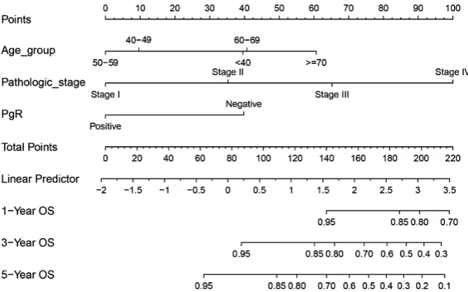
(VI) Draw the Nomogram based on the Cox model. The survival function object is calculated at 1-, 3-, and 5-year (12, 36, and 60 months, respectively). Lp (Linear prediction) is set to FALSE to suppress creation of an axis for scoring X beta. Maxscale means the highest points (Figure 1).
nom<-nomogram(coxm,fun=list(function(x) surv(12, x), function(x) surv(36, x), function(x) surv(60, x)),lp = T,funlabel = c('1-Yeas OS', '3-Year OS','5-YearOS'),maxscale = 100, fun.at = c('0.95','0.85','0.80','0.70','0.6','0.5','0.4','0.3','0.2','0.1'))
plot((nom), xfrac = .3)
(VII) Now, by drawing a straight line down to the axis of points and survival rates for each independent variable, the corresponding points of these factors of each patient can be calculated in total, which will be located on the survival axis with a perpendicular line. However, when there are several variables and a large number of patients, it will be a large and tedious task to calculate the total points and survival rates for each of those patients. Meanwhile, because the break of scale in the axis is 50 points per unit, there will also be a non-negligible systematic error derived from it. In such circumstances, a precise formula behind the Nomogram plot that serves as a “bridge” between the Cox model and the Nomogram is warranted. The package “nomogramEx” provides this function.
nomogramEx(nomo=nom,np=3,digit=3)
[image:3.595.129.463.84.292.2]“Nomo” indicates the Nomogram object mentioned above. “Np” means the number of predictions in the
nomogram. We predicted 1-, 3- and 5-year, then np =3.
“Digit” defines the number of decimal digits; the default is 9.
The prediction would be more precise if this parameter was set larger, but if so, the time needed for calculation would increase.
> nomogramEx(nomo=nom,np=3,digit=3) $RESULT
[1] "The equation of each variable as follows:" [[2]]
Age_group 1 39.562906 2 60.689474 3 9.585177 4 0.000000 5 40.759591 [[3]]
Pathologic_stage 6 0.00000 7 35.27158 8 65.21458 9 100.00000 [[4]]
PgR 10 39.79384 11 0.00000 [[5]]
[1] "1-Year OS = 0 * points ^3 + 0 * points ^2 + -0.009 * points + 1.395"
[[6]]
[1] "3-Year OS = 0 * points ^3 + 0 * points ^2 + 0.005 * points + 0.749"
[[7]]
[1] "5-Year OS = 0 * points ^3 + 0 * points ^2 + 0.011 * points + 0.594"
Now, the assignment of points for each level of each variable and the formula for overall survival rates in 1-, 3-, and 5-year overall survival probabilities are displayed in the result.
(VIII) Furthermore, with the assistance of the package “nomogramFormula,” we can automatically calculate the total points and survival probabilities for each patient in the original data with the
formula_lp function in this package.
#get the formula of total points by the best power using formula_lp
options(oldoption)
results <- formula_lp(nomogram = nom)
points<-points_cal(formula = results$formula, lp = f$linear. predictors)
head(points)
#Then calculate the survival probabilities prob<-prob_cal(reg = coxm,times = c(12,36,60)) head(prob)
#Finally integrate the calculation results into the original dataframe.
breast$points<-points breast<-cbind(breast,prob) head(breast)
> head(breast)
No Months Status Age ER PgR Margin_status Pathologic_stage HER2_Status
9 9 8.633333 0 70 Positive Negative Nagative Stage I Negative
11 11 44.033333 0 56 Positive Positive Nagative Stage I Negative
12 12 48.766667 0 54 Positive Positive Nagative Stage II Negative
13 13 14.466667 0 61 Positive Positive Nagative Stage II Negative
14 14 47.900000 0 39 Negative Positive Nagative Stage II Negative
19 19 39.866667 0 50 Positive Positive Nagative Stage II Positive
Menopause_status Surgery_method Histological_type Age_group points
9 Post menopause Lumpectomy Other >=70 100.483316
11 Pre menopause Modified Radical Mastectomy Other 50-60 0.000001
12 Pre menopause Modified Radical Mastectomy Infiltrating Ductal Carcinoma 50-60 35.271582
13 Post menopause Lumpectomy Other 60-70 76.031173
14 Pre menopause Lumpectomy Infiltrating Ductal Carcinoma <40 74.834488
19 Post menopause Lumpectomy Infiltrating Ductal Carcinoma 50-60 35.271582
11 -1.93379523 0.9984382 0.9940269 0.9892102 12 -1.05408170 0.9962400 0.9856642 0.9741919 13 -0.03749093 0.9896426 0.9608785 0.9302855 14 -0.06733762 0.9899456 0.9620068 0.9322644 19 -1.05408170 0.9962400 0.9856642 0.9741919
Now, the total points and corresponding survival probabilities for 1-, 3-, and 5-years (named as P12, P36, and P60 because the units for survival time were set as months) are then displayed in the original data frame.
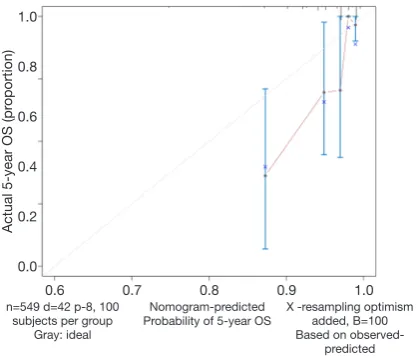
(IX) Calculate the C-index and draw the calibration curve as suggested (Figure 2).
C-index
f<-coxph(Surv(Months,Status==1) ~ Age_group+Pathologic_ stage+PgR, data = breast)
sum.surv<-summary(f)
c_index<-sum.surv$concordance c_index
> c_index C se(C)
0.79143349 0.04012905
Calibration curve
cal<- calibrate(coxm, cmethod = 'KM', method = 'boot', u = 60, m = 100, B = 100)
plot(cal,lwd=2,lty=1,errbar.col=c(rgb(0,118,192,maxColor Value=255)), xlim=c(0.6,1), ylim=c(0.6,1), xlab='Nomogram-Predicted Probability of 5-Year OS', ylab='Actual 5-Year OS(proportion)', col=c(rgb(192,98,83,maxColorValue=255))) lines(cal[,c('mean.predicted','KM')],type='b',lwd=2, col=c(rgb( 192,98,83,maxColorValue=255)), pch=16)
abline(0,1,lty=3,lwd=2,col=c(rgb(0,118,192,maxColorVal ue=255)))
As shown in the result, the C-index of our model equals 0.7914, which is higher than that (0.7503) in the article by Zhou et al. (3), indicating the better predicting value of
our model and thus displaying the priority of defining age
and pathologic stage as categorical rather than continuous
variables. We can find that patients with 40–59 years of age
have the best survival while the risk of the younger patients with <40 years of age greatly increases.
In summary, based on the detailed and comprehensive interpretation of the “ins and outs” of Nomogram in this article, we provide an approach to make this methodology more simplified and accurate. We would like to express our sincere appreciation to Dr. Zhou for his efforts in this article. His work has served as the best tutorial and
reference in the field of statistics for researchers wanting to
conduct clinical studies.
Acknowledgments
We thank the International Science Editing Co. (http:// www.internationalscienceediting.com) for grammatically editing this manuscript.
Footnote
Conflicts of Interest: The authors have no conflicts of interest
to declare.
Ethical Statement: The authors are accountable for all aspects of the work in ensuring that questions related to the accuracy or integrity of any part of the work are appropriately investigated and resolved.
References
1. Djulbegovic B, Guyatt GH. Progress in evidence-based medicine: a quarter century on. Lancet 2017;390:415-23. 2. Reza Soroushmehr SM, Najarian K. Transforming big
data into computational models for personalized medicine
1.0
0.8
0.6
0.4
0.2
0.0
0.6 0.7 0.8 0.9 1.0
Actual 5-year OS (pr
oportion)
n=549 d=42 p-8, 100 subjects per group
Gray: ideal
Nomogram-predicted
Probability of 5-year OS X -resampling optimism added, B=100 Based on
[image:5.595.63.272.83.262.2]observed-predicted
and health care. Dialogues Clin Neurosci 2016;18:339-43. 3. Zhou ZR, Wang WW, Li Y, et al. In-depth mining of
clinical data: the construction of clinical prediction model with R. Ann Transl Med 2019;7:796.
4. Han K, Song K, Choi BW. How to Develop, Validate, and Compare Clinical Prediction Models Involving Radiological Parameters: Study Design and Statistical Methods. Korean J Radiol 2016;17:339-50.
5. Steyerberg EW, Vergouwe Y. Towards better clinical prediction models: seven steps for development and an ABCD for validation. Eur Heart J 2014;35:1925-31. 6. Woodward M, Tunstall-Pedoe H, Peters SA. Graphics and
statistics for cardiology: clinical prediction rules. Heart 2017;103:538-45.
7. Iasonos A, Schrag D, Raj GV. How to build and
interpret a nomogram for cancer prognosis. J Clin Oncol 2008;26:1364-70.
8. Bochner BH, Kattan MW, Vora KC. Postoperative
nomogram predicting risk of recurrence after radical cystectomy for bladder cancer. J Clin Oncol 2006;24:3967-72.
9. Bi G, Lu T, Yao G, et al. The Prognostic Value Of Lymph Node Ratio In Patients With N2 Stage Lung Squamous Cell Carcinoma: A Nomogram And Heat Map Approach. Cancer Manag Res 2019;11:9427-37.
10. Deng W, Xu T, Xu Y, et al. Survival Patterns for Patients with Resected N2 Non-Small Cell Lung Cancer and Postoperative Radiotherapy: A Prognostic Scoring Model and Heat Map Approach. J Thorac Oncol 2018;13:1968-74. 11. Du Z, Hao Y. R package "nomogramEx". Available online:
https://cran.r-project.org/web/packages/nomogramEx/ index.html
12. Zhang J, Jin Z. R package "nomogramFormula". Available online: https://github.com/yikeshu0611/ nomogramFormula