Coverage prediction and optimization algorithms for indoor environments

R E S E A R C H

Open Access

Coverage prediction and optimization algorithms

for indoor environments

David Plets

, Wout Joseph, Kris Vanhecke, Emmeric Tanghe and Luc Martens

Abstract

A heuristic algorithm is developed for the prediction of indoor coverage. Measurements on one floor of an office building are performed to investigate propagation characteristics and validations with very limited additional tuning are performed on another floor of the same building and in three other buildings. The prediction method relies on the free-space loss model for every environment, this way intending to reduce the dependency of the model on the environment upon which the model is based, as is the case with many other models. The

applicability of the algorithm to a wireless testbed network with fixed WiFi 802.11b/g nodes is discussed based on a site survey. The prediction algorithm can easily be implemented in network planning algorithms, as will be illustrated with a network reduction and a network optimization algorithm. We aim to provide an physically intuitive, yet accurate prediction of the path loss for different building types.

1. Introduction

The increasing use of indoor wireless systems in office buildings, exhibition halls, factories, ... gives rise to a need for indoor propagation prediction models that can be used for different building types, with a sufficient accuracy. Information about the geometry and physical properties of the buildings allow obtaining better predic-tions than a classical one-slope log-distance model. The characterization of path loss in indoor environments has been the subject of extensive research and many models have been proposed to make accurate predictions. Indoor propagation and wireless prediction tools have been investigated in [1-25]. Statistical models are easy to obtain when a lot of measurement data is available, but their validity is limited to the category of buildings they represent. Ray-tracing tools therefore take into account the geometry of the building and the used materials. However, the results appear to be very dependent on geometrical details of the ground plan, which force the user to work with very accurate plans. The number of included interactions (transmissions, reflections, and dif-fractions) also have a huge influence on the predicted path loss: as will be shown in this article, differences up to 5 dB have been observed for the average path loss along a line-of-sight (LoS) path when the number of

interactions is adjusted (see Section 9). Finally, for a high number of interactions, calculation time of ray-tracing tools may run to a range of days (on a computer with an Intel Xeon-3400 single-core 3.4 GHz processor with 4 GB DDR2-SDRAM).

In this article, an algorithm for indoor path loss pre-diction at 2.4 GHz is proposed, avoiding the problems of both methods mentioned above. It is based on the calculation of the dominant path between transmitter and receiver [10]. Measurements have been performed in four buildings in Belgium for constructing and vali-dating the model. A comparison with ray-tracing simu-lations is executed. The applicability to an actual wireless testbed network is investigated. Furthermore, an algorithm for the reduction of the number of access points of a network is presented. Since networks are often overdimensioned, especially in office environ-ments, this algorithm could aid in reducing operating costs. Then, a network optimization algorithm is dis-cussed. This algorithm can be of great interest to any-one who wants to set up a new WiFi or sensor network in either home or professional environments. It allows meeting a certain throughput requirement with a mini-mum number of transmit nodes.

Section 2 discusses related study and available litera-ture. In Section 3, the concept and the objectives of the research are explained, followed by a description of the buildings and their use in the propagation modeling * Correspondence: david.plets@intec.UGent.be

Department of Information Technology, Ghent University/IBBT, Gaston Crommenlaan 8 box 201, B-9050 Ghent, Belgium

procedure in Section 4. In Section 5, the measurement setup is described, and in Section 6, the prediction algo-rithm is presented. The modeling of the path loss para-meters is discussed in Sections 7 and 8 investigates different validation cases. Section 9 provides a compari-son of the proposed model with results from a ray-tra-cing tool. In Section 10, the applicability of the model to a wireless testbed is discussed. Section 11 presents an algorithm for reducing the number of access points and Section 12 an algorithm for network optimization. Finally, conclusions are presented in Section 13.

2. Related study

Indoor propagation has been the subject of many research studies. These studies describe either ray mod-els [1-5], numerical solver modmod-els [6-9], heuristic predic-tions [10-13], statistical (site-specific) models [14-22], or specific propagation aspects [23-25]. Our algorithm can be classified as heuristic. Heuristic predictions are based on one or more rules of thumb in order to make an accurate yet fast prediction for the path loss. Ray-tracing and ray-launching model techniques usually require a vector based description of the environment to identify the reflected and diffracted rays from surface and edges [26]. Statistical (site-specific) models predict path loss based on measurements for a specific site or for a speci-fic environment, limiting the validity of the prediction to the propagation environment it represents. Numerical solver models consist of screen or integral methods, Finite-difference time-domain (FDTD), ... [26].

In [1], ray-tracing is used for indoor path loss predic-tion, with a distinction between LoS and NLoS. Procen-tual prediction errors range from 5% to 10%, which is higher than for our algorithm. Different ray-tracing approaches (field-sum and power-sum) have been inves-tigated in [4]. Field-sum appeared to be most accurate. In [2,3], efficient two-dimensional ray-tracing algorithms for an indoor environment have been presented, result-ing in a significant reduction in the computational time, without losing prediction accuracy.

A theoretical waveguide model permitting a rigorous modal solution is proposed for predicting path loss inside buildings in [6].

Heuristic approaches have been proposed in [11-13]. An indoor propagation model making use of the estima-tion of the transmitted field at the corners of each room is presented in [11]. The performance is comparable to that of our algorithm (mean absolute prediction error of 2.17 dB), but the model is only tested for simple config-urations, with (ideally) at most one wall between trans-mitter and receiver. Only the direct ray is considered, which makes the model less suitable for environments where diffraction is the dominant mechanism. More-over, only one path loss value is obtained for the whole

room, based on the values in the corners of the room. This makes the predictions less accurate for concave rooms or rooms with a non-rectangular shape. A more complex version of the dominant path loss model (using more model parameters) is studied in [12]. In the study, the model parameters are calibrated in order to mini-mize the prediction errors in a certain building. Good results are obtained, but no validation measurements have been performed in other buildings, limiting the validity of the model to the investigated building.

Different statistical models for specific environments have been proposed. In [14], indoor path losses have been statistically investigated for different room cate-gories (adjacent to transmitter room, non-adjacent, ...) in 14 houses. Path losses in five office environments have been determined and the importance of taking wall attenuations into account in the prediction model is indicated in [15]. In [17], low prediction errors are obtained, but the analysis was performed for a site-spe-cific validation of the ITU indoor path loss model (only indoor office environments). In [19], different propaga-tion models were tuned to a measurement set, but no validation measurements were performed. One-slope models and different multi-wall based models were ana-lyzed and results have been provided for a typical office environment in [27]. The standard deviation of the model error was around 6 dB for the best model. In [20], a simple one-slope model was constructed for a mostly-LoS environment. A value of 2 for the parameter

n(see Equation (1)) was obtained. LoS and NLoS mea-surements have been fitted to a one-slope model in [22], where the path loss exponent accounted also for the wall losses for the NLoS measurements. However, no model validations in other rooms or buildings were exe-cuted. In [21], a statistical path loss model is proposed for different propagation conditions. The use of statisti-cal models is however restricted to the category of buildings the model was constructed for, limiting the general applicability of the model. Moreover, no valida-tion measurements have been performed to test the model.

In [23], upper and lower limits for LoS transmission at 1.8 GHz were investigated. It was found that these were influenced by ceiling height and antenna height.

suppliers, in indoor and outdoor environments. The indoor propagation algorithm used in [13] uses the indoor dominant path model (IDP) [10]. The presented prediction results (at one test site) have a variable accuracy.

3. Concept and objective

A heuristic algorithm taking into account the effect of the environment on the wireless propagation channel, has been developed for the prediction of the path loss (see Section 6) in zones of about 5 m2. The dominant path is determined with a multidimensional optimiza-tion algorithm that searches the lowest total path loss, consisting of a distance loss (taking into account the length of the propagation path), a cumulated wall loss (taking into account the walls penetrated along the pro-pagation path), and an interaction loss (taking into account the propagation direction changes of the path, e.g., around corners). Measurements on one floor of an office building have been performed to investigate pro-pagation characteristics. The wall penetration losses have been determined from measurements and literature [28] and interaction loss has been fitted to match these measurements. Measurements on another floor of the same building and in three other buildings have been executed to validate the model with limited additional tuning. Our prediction method relies on the free-space loss model for every environment, this way intending to reduce the dependency of the model on the environ-ment upon which the model is based, as is the case with many other models or tools. The applicability of the algorithm to a wireless testbed network with fixed WiFi 802.11b/g nodes is discussed based on a site survey with signal strength measurements. The prediction algorithm can easily be implemented in network planning algo-rithms, as will be illustrated with a network reduction and a network optimization algorithm. We aim to pro-vide an physically intuitive, yet accurate prediction of the path loss for different types of public and office buildings.

4. Investigated buildings

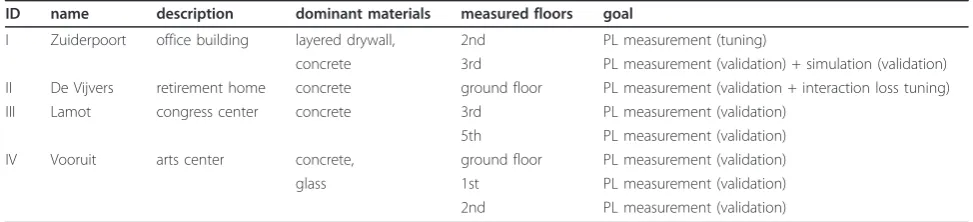
In this article, an indoor path loss model for the accu-rate calculation of WLAN coverage will be formulated. To determine the model parameters, PL measurements and simulations have been performed in four very differ-ent buildings, named Zuiderpoort (I), De Vijvers (II), Lamot (III), and Vooruit (IV). The characteristics of the investigated buildings are described hereafter and are summarized in Table 1 at the end of this section.

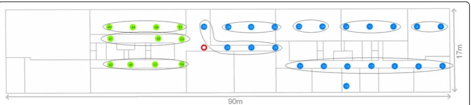
Zuiderpoort is a modern three-storey office building, with movable walls (layered drywalls) around a core consisting of concrete walls (Table 1). Figures 1 and 2 show (a part of) the second floor and the (entire) third

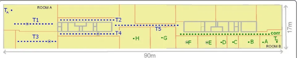
floor, respectively. Path loss measurements have been performed on both floors (1,581 path loss samples on the second floor and 5,078 samples on the third floor), path loss simulations (with the ray-tracing tool Wireless InSite®from Remcom) only for the third floor. The orange walls are layered drywalls, the grey ones are made of concrete. In order to assure the validity of the predictions for the entire building floor, trajectories T1-T5 are chosen to represent LoS, obstructed line-of-sight (OLoS), as well as NLoS propagation cases, while rooms A-H are chosen to investigate propagation through sub-sequently adjacent rooms. In rooms A-H, an average path loss in the room is calculated by moving the recei-ver antenna randomly through the room during 2 min. For the measurements on the third floor (Figure 2), TA is the access point for measurement trajectories T1-T5 and TBfor measurements in rooms A-H and for mea-surement trajectory‘corr’(corridor).

De Vijvers is a retirement home (Table 1), where 7,095 measurement samples were collected along twelve trajectories (T1-T12) on the ground floor (see Figure 3). The building mainly consists of concrete walls. Both LoS and NLoS trajectories are chosen to investigate the path loss prediction. For trajectory T1 (purple rectangle) the purple indicated transmitter (TA, purple dot) was active, for trajectories T2-T12 (blue rectangles) the blue indicated transmitter (TB, blue dot).

Lamot is a multi-storey congress and heritage center with multipurpose rooms for conferences, seminars, workshops, fashion shows, product presentations, .... Thirteen path loss measurement trajectories (4,070 sam-ples) have been executed on the third floor and the fifth floor, both having a similar geometry. The building is mainly constructed with concrete walls. Both LoS and NLoS trajectories are chosen to investigate the path loss prediction.

Vooruit is a polyvalent arts center for all kinds of events (concerts, parties, debates, ...), built between 1911 and 1914. Measurements are performed on three floors (ground floor, first floor, and second floor). This build-ing also mainly consists of concrete walls, some of them even with a thickness of 50 cm. Seventeen trajectories (4,390 samples) have been traversed for the path loss measurements in this building. Mostly, NLoS predic-tions are chosen to investigate the path loss prediction.

It is clear that these buildings have very different char-acteristics. It will be shown that our approach is capable to predict path loss for these different indoor environments.

5. Path loss measurements

section discusses the setup for these path loss measure-ments and their reproducibility.

5.1. Measurement setup

As Tx an omnidirectional Jaybeam antenna type MA431Z00 with a gain of 4.2 dBi is used. The Tx is placed at a height of 2.5 m above ground level (typical access point height in public environments). It is fed with a continuous sine wave at 2.4 GHz (ISM-band, typical for WLAN communication) with an EIRP of 20 dBm. Possible interfering sources (e.g., WiFi networks) are deactivated in order not to influence the measure-ments. The receiver antenna (identical to Tx) is attached to a cart at a height of 1 m (typical user device height) and is connected to a Rohde & Schwarz FSEM30 spec-trum analyzer with a frequency range from 20 Hz up to 26.5 GHz. The output of the SA is sampled and stored

on a laptop used to record and process the measure-ment data. The models have been constructed for omni-directional antenna radiation patterns. Access points mostly have simple monopole or dipole antennas.

5.2. Reproducibility

Since the model parameters are based almost solely on the path loss measurements performed on the second floor of the Zuiderpoort building, it is important that the measured path loss values are reliable. Therefore, we investigate the reproducibility of the measurements by executing them four times for each of the five trajec-tories (three times for T2 due to practical reasons). Figure 1 shows these five measurement trajectories (green squares) with the indication of the access point (blue circle with dot) on the ground plan of (a part of) the second floor. The predicted path loss is

Table 1 Overview of the characteristics of the investigated buildings

ID name description dominant materials measured floors goal

I Zuiderpoort office building layered drywall, 2nd PL measurement (tuning)

concrete 3rd PL measurement (validation) + simulation (validation) II De Vijvers retirement home concrete ground floor PL measurement (validation + interaction loss tuning) III Lamot congress center concrete 3rd PL measurement (validation)

5th PL measurement (validation) IV Vooruit arts center concrete, ground floor PL measurement (validation)

glass 1st PL measurement (validation)

2nd PL measurement (validation)

superimposed on the floor plan using a colour code, explained in the figure caption.

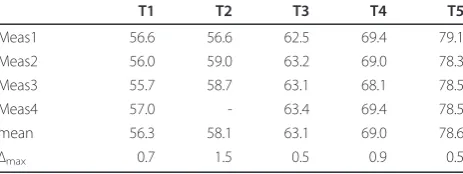
Table 2 shows the average path loss recorded along T1-T5 for the four measurements (Meas1 to Meas4). Table 2 shows that the maximum deviation from the average path loss Δmax varies only from 0.5 dB to 1.5 dB, indicating that one measurement suffices to give a correct estimate of the path loss along a trajectory. These average values will be used to determine the model parameters in Section 7.

6. Algorithm concept and implementation

In this section, the concept and the implementation of the prediction algorithm is discussed. Our goal is to develop an accurate and fast algorithm that does not make use of extensive fitting to obtain good predictions, as this often leads to results which are only usable for the investigated building.

The planning algorithm predicts the indoor coverage by means of path loss prediction based on the IDP [10]. This model is a compromise between semi-empirical models only considering the “direct”ray between trans-mitter Tx and receiver Rx (e.g., Motley-Keenan multi-wall model [29]) and ray-tracing models where hundreds of rays and their interactions with the environment are investigated. In the IDP model, propagation focuses on the dominant path between transmitter and receiver, i. e., the path along which the signal encounters the smal-lest obstruction in terms of path loss. It takes into account the length along the path, the number and type of interactions (e.g., reflection, transmission, etc.), the material properties of the objects encountered along the path, etc. The approach of using the IDP model is justi-fied by the fact that more than 95% of the energy received is contained in only 2 or 3 rays [10]. According to [10], predictions made by IDP models reach the accu-racy of ray-tracing models or even exceed it. In Section 9, model predictions will be compared with ray-tracing tool predictions.

Different propagation properties can be chosen to be included into the IDP model. We have chosen to take

into account the distance along the dominant path (distance loss), the corresponding wall losses, and the propagation direction changes along the dominant path (interaction loss). The IDP model as presented in [30] also adds other factors, such as waveguiding, transmit-ter room size, .... The more factors used though, the more tuning is needed (limited general use) and the more difficult it is to determine the influence of each single factor on the path loss. As a result, neural net-works are mostly needed to construct a path loss model. Also, the more influencing factors included, the higher the dimensions of the problem, and the more training patterns needed to construct reliable models. Therefore, we aimed to construct a model as simple as possible, but as complex as necessary for accurate pre-dictions, this way improving the IDP model from [10,30]. In Sections 7 and 8, it will be demonstrated that the proposed three contributing factors suffice to perform solid predictions.

6.1. General path loss model

The path loss model, based on the three discussed con-tributions (distance loss, cumulated wall loss, interaction loss), will now be discussed. Path losses are determined between the transmit antenna of an access point and a receiving antenna at a certain location. These receiver points are located on a grid, of which the grid resolution can be set as a parameter by the user (e.g., 2 m).

The total path loss of a certain path can thus be calcu-lated as follows:

PL = PL0+ 10 n log

d d0

distance loss

+

i

LWi

cumulated wall loss

+

j

LB,j

interaction loss

,

(1)

where PL [dB] is the total path loss along the path, PL0[dB] is the path loss at a distance of d0 according to Figure 3Ground plan of‘De Vijvers’with indication of transmitters (blue and purple dots), measurement trajectories (blue and purple rectangles). The points for which the different path loss contributions are investigated in Table 3 are indicated on T3, T4, and T6 with a black dot within a white dot.

Table 2 Reproducibility of the measured path loss along T1-T5

T1 T2 T3 T4 T5

Meas1 56.6 56.6 62.5 69.4 79.1

Meas2 56.0 59.0 63.2 69.0 78.3

Meas3 55.7 58.7 63.1 68.1 78.5

Meas4 57.0 - 63.4 69.4 78.5

mean 56.3 58.1 63.1 69.0 78.6

the distance loss model, d [m] is the distance along the path between access point and receiver, d0 [m] is a reference distance, and n [-] is the path-loss exponent. d0was chosen 1 m here. The first two terms of the sum represent the path loss due to the distance along the considered path, noted here as the “distance loss”. It is calculated for a certain path as the path loss at a distance equal to the length of the path that traverses all the walls of the considered path.

i

LWiis the“

cumu-lated wall loss” along the path (i.e., the sum of the wall lossesLWiof all walls Wi traversed along the path,

i= 1, ..., W, whereWis the total number of walls along

the path).

j

LBj_{is the}“interaction loss”, i.e., the

cumu-lated lossLBjcaused by all propagation direction changes

Bjof the propagation path from access point to receiver, with j = 1, ...,B, whereB is the number of times the propagation path changes its direction. Values for the model parameters will be determined in Section 7. Typi-cal contributions of the distance loss, cumulated wall loss, and interactions loss for different transmitter-recei-ver configurations will be presented in Section 3.

6.2. Search algorithm for dominant path

The dominant path is defined as the path for which the sum of the cumulated wall loss, the distance loss, and the interaction loss is the lowest. We assume thus that this path represents almost the total energy. The minimization is performed by a multi-dimensional optimization algorithm. In the following, the algorithm used for the determination of the dominant path is discussed.

The path loss between an access point and a grid point is determined by calculating the path lossfor all

possible paths between access point and grid point,

where optimizations are implemented in order to speed up the calculations. Figure 4a shows an example ground plan of a floor level, where the paths from a random grid point in room 3 (marked with a black dot) to the access point (in room 4) are determined. A tree is cre-ated with as root the room in which the investigcre-ated grid point is located (e.g., room 3 of Figure 4a,b). Each branch corresponds to a wall connecting two rooms with as weight the wall loss between both rooms. For each new room in the tree, new branches are originated. This tree represents the possible paths between an access point and the receiver. Figure 4b shows the tree (from receiver Rx to access point AP) corresponding with the ground plan of Figure 4a for the proposed algorithm. In both figures, the rooms are indicated with numbers in squares, and the walls with letters in circles. The tree here yields the following paths, consisting of a sequence of walls to reach room 4 from room 3: B-A-F, B-E, B-D-G, C-G, C-D-A-F, C-D-E. For reasons of

clarity, exterior walls are not included in the tree in Figure 4b, since they always lead to the termination of a certain branch. Each time the room with the access point is reached, the total loss is calculated (distance loss + cumulated wall loss + interaction loss). If the total loss for this new path is lower than the current lowest loss, then the best path is updated. In order to find a path as quickly as possible, the branches are added so that the walls closest to the access point are added first. Because the tree is built in a “depth-first” way, the algorithm leads to a solution as fast as possible. This also allows the algorithm to prematurely end branches where the room of the access point could not be reached with a path loss that is lower than the path loss that is currently the lowest, this way reducing the calculation time of the algorithm.

6.2.1. Determination of the physical path between access point and receiver

The algorithm could easily be extended to propagation between different floors. However, we chose not to implement this (yet), because in most (office and public) environments, access points are not supposed to provide coverage on other floors.

6.3. Physical rationale: judiciously chosen and physically intuitive path

Our model was aimed at an intuitive understanding of how path loss is affected, without losing accuracy. The three contributions taken into account in the model of Equation (1) (distance loss, cumulated wall loss, and interaction loss) are selected based on the real physical propagation of a wave between transmitter and receiver. The well-known Motley-Keenan multi-wall model [29] in contrast to our model, calculates the loss experienced along thedirect raybetween transmitter and receiver: it is indeed clear that an increasing distance and a higher number of walls between Tx and Rx (first two factors of Equation (1)) lead to a higher path loss, but this model is not realistic for all situations. We illustrate this with the following example of a configuration of a transmitter and a receiver, both placed in a corridor making a 90° turn around a reinforced concrete block (Figure 5). In reality, the wave will propagate along the corridor (dif-fract at the corner point), instead of propagating through the three walls. The power received from the direct ray between Tx and Rx will thus be much lower,

meaning the Motley-Keenan model will overestimate the actual path loss. To cope with similar situations, a third contribution factor, the interaction loss, is introduced, taking into account propagation direction changes of the path in our model. Interaction loss is also used in the IDP model in [10].

To gain more insight into the proposed model, we will now investigate the contributions to the total path loss of the three factors, namely distance loss, cumulated wall loss, and interaction loss, for eight different trans-mitter-receiver configurations: five points circled in Figure 2 on the third floor of the Zuiderpoort building,

(a) (b)

Figure 4Example of building floor with (a) ground plan (rooms 1-5, walls A-G, AP = access point, Rx = receiver, midpoints a-g) with indication of three possible paths and (b) tree yielding all possible paths from room 3 to room 4.

and three points indicated with a black dot within a white dot in Figure 3 in the building of De Vijvers.

Table 3 shows the three different contributions to the total path loss between the transmit antenna and each of these pointsPB_T, where B indicates the building where the point is located (Z= Zuiderpoort orV= De Vijvers) and T indicates the trajectory on which or the room in which the point is located. The table also shows the dominant path from transmitter to receiver. Different propagation situations are illustrated: LoSPZ

T1

, OLoS with onePZ_T3or morePZ_Ewalls between Tx and Rx, and propagation through corridors and/or rooms (all other points). In all cases, the distance loss is by far the most dominant factor. When the cumulated wall loss increases, it becomes more likely that another path (through corridors) will be dominant. In the De Vijvers building (containing a lot of concrete walls), the interac-tion losses can be quite high (up to 17.2 dB forPV

T4).

7. Modeling the parameters of the dominant path model

In this section, the model parameters will be deter-mined. The four buildings described in Section 4 are used for the construction and the validation of the path loss model. We have deliberately chosen different types of buildings (modern office building, retirement home, modern congress center with large exhibition halls, and old arts center), in order to investigate the general applicability of the model. Path loss measurements on the different investigated building floors are used either for tuning the model parameters or for validation pur-poses (see Table 1, column‘goal’).

7.1. Distance loss

A first limitation we impose ourselves is the use of the free-space loss model for thedistance loss (see Equa-tion (1):n= 2, PL0 = 40 dB, d0 = 1 m), because we aim to use a general model, avoiding fitting and tuning of

the model to agree with existing measurement data of a certain environment. This way, we intend to increase the general applicability of Equation (1). Changing these parameters might probably improve the prediction accu-racy in the model tuning phase, but it is more likely that the resulting model would be too specific for a spe-cific building (type), something we try to avoid in this research. The free-space loss model seemed like a good starting point for a general prediction model. Results will indicate that this was a feasible choice.

7.2. Cumulated wall loss

For the determination of the term representing the cumulated wall loss (see Equation (1), we have first measured the penetration loss of the two wall types present in the Zuiderpoort building, layered drywalls (orange walls in Figure 2) and concrete walls (grey walls in Figure 2), and we have used the (rounded) values in the model, 2 dB and 10 dB, respectively. For other wall types, we have based the loss values on available litera-ture (e.g., [28]). For glass (windows or glass doors) 2 dB was used. The importance of correct wall penetration loss values is demonstrated in [26]. Table 4 lists the used values for the penetration losses for thin (< 15 cm) and thick (> 15 cm) walls composed of different material types. We limit this table to the most occurring building materials. The table can easily be extended with

Table 3 Overview of the three different contributions (DL = Distance Loss, CWL = Cumulated Wall Loss,

IL = Interaction Loss) to the total path loss PL between eight receiver points and the transmitter in two buildings

Rx Tx DL CWL IL PL Dominant path

point [dB] [dB] [dB] [dB]

T3 TB 75.2 2.0 17.0 94.2 through corridors along T2 and T3 PV

T4 TB 78.7 2.0 17.2 97.9 through corridors along T2, T3, and T4 PV

T6 TB 73.8 6.0 15.0 94.8 through corridor along T2, then crossing the inner yard

then crossing the inner yard

Table 4 Penetration losses used in the prediction model

penetration losses for various other materials using results from additional measurements or numbers and tables of [31,32].

7.3. Interaction loss

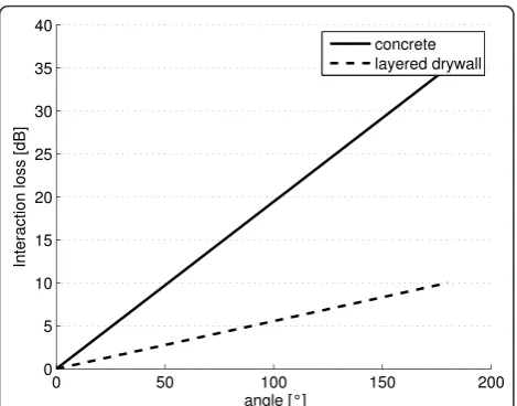
Based on the contribution of the distance loss and wall loss factor obtained as explained above, the value of the third factor, the interaction lossfactor (see Equation (1), was adjusted in order to match the predictions to measurements performed on the second floor of the Zuiderpoort building. The measurements on this build-ing floor were thus used to tune the model (see Table 1, column‘goal’) and allowed us to determine the relation between the angle made by a propagation path and the additional loss associated with the propagation direction change. Because the interaction loss should be the same for e.g., three changes of 30° and one change of 90°, a linear relationship is proposed.

LB,j= A· ˆBj (2)

where LB,j[dB] is the loss caused by bend Bj, A [dB/°] is a parameter depending on the dominant material in the building andBˆj[◦]is the angle corresponding with

bend Bj. Based on measurements in two perpendicular corridors, A was determined at 0.0556 dB/° or 5 dB/90° for the Zuiderpoort (see Figures 1 and 2) building, con-sisting mainly of layered drywalls. Figure 6 shows the obtained relationship between the angle of the bend made by the propagation path and the corresponding interaction loss of Equation (2) for layered drywalls.

7.4. Parameter values for the buildings used for validation

With the model parameters for distance loss, cumulated wall loss, and interaction loss now fixed, measurements on the third floor of the Zuiderpoort building were per-formed as a first validation without any further tuning (see Table 1), albeit in a very similar environment.

However, for the De Vijvers building, an environment mainly consisting of concrete walls (versus the lighter layered drywalls in the Zuiderpoort building), the loss when propagating around corners appeared to be higher than for the Zuiderpoort building. The interaction loss for this environment was tuned to a value of 0.1946 dB/ ° or 17.5 dB/90° for concrete walls (see Figure 6, ‘con-crete’). In fact, it was only tuned for one of the twelve trajectories (T5, a trajectory where the dominant path made a propagation direction change), so all other mea-sured trajectories in this building can be considered as validation trajectories as well (see Table 1, column ‘goal’).

For the remaining two buildings (Lamot and Vooruit), all model parameters from the analysis of the Zuider-poort and De Vijvers buildings were used unchanged. Both buildings mainly consist of concrete, so we could immediately use the interaction loss function from the De Vijvers building (see‘concrete’in Figure 6), and vali-date the model with new measurements, without any additional tuning. Sections 7 and 8 will demonstrate that these validation results are more than satisfactory. Table 1 summarizes the goal (model tuning and/or vali-dation) of the measurements in the different buildings.

For new environments with similar building materials, we advise to use the parameters as derived above. How-ever, when other materials are used, it is important to determine their correct penetration loss value [26]. Also, the interaction loss function could vary for new environ-ments, e.g., in buildings with a lot of glass or metal walls. In that case, the interaction loss function could be determined by executing a limited path loss measure-ment in two perpendicular corridors. It is expected that, compared to concrete materials, interactions losses are lower for glass materials, but higher for metal walls.

7.5. Model performance for second floor of Zuiderpoort building

The model of Equation (1) with its parameters chosen as explained above is first used to calculate the devia-tions between the predicdevia-tions and the measurements for the second floor of the Zuiderpoort building.

Table 5 shows for all trajectories on the second floor (used for modeling) the measured average path loss PLms [dB], the predicted path loss PLpr, and the deviationδ[dB]

0 50 100 150 200

for the considered model for Tx and Rx at heights of 2.5 m and 1 m, respectively.δ[dB] is defined as follows.

δ[dB] = PLpr[dB]−PLms[dB] (3)

Small deviations are obtained in Table 5 for the sec-ond floor of the Zuiderpoort building. This is to be expected, since this is the building floor that was used for model tuning purposes. The average of the absolute value of the deviation |δ| is 1.77 dB for the second floor. The deviation δhas an average of -1.15 dB with a stan-dard deviation of 2.33 dB. Values for the stanstan-dard devia-tion of 3 dB to 6 dB are considered to be excellent according to [26]. Our prediction algorithm performs better than this requirement.

8. Validation of path loss model with measurements in other buildings

The parameter values of our prediction algorithm are based on measurements on one floor of one building (second floor, Zuiderpoort, see Section 7). In this sec-tion, we validate the general applicability of our method by firstly comparing with measurements on another floor of the Zuiderpoort building and secondly, with measurement results from three other buildings.

8.1. Validation cases

The measurement trajectories on the third floor of the Zuiderpoort building(see Figure 2) serve as a first vali-dation for the model proposed in Section 7 (based on measurements on second floor of Zuiderpoort building). Table 5 summarizes for all trajectories on the third floor (T1-T5, A-H, and corr) the measured average path loss PLms[dB], the predicted path loss PLpr, and the devia-tionδ[dB] = PLpr - PLmsfor the considered model for Tx and Rx at heights of 2.5 m and 1 m, respectively. An average value for the absolute deviations (|δ|) on the third floor is only 2.56 dB. The mean of the deviationsδ for the whole third floor is -0.24 dB with a standard deviation of 3.47 dB. This shows that the obtained pre-diction model is valid for a similar propagation environ-ment (same building, but other floor, similar materials used) without tuning of the parameters in contrary to, e.g., [33].

The measurement campaign of twelve trajectories on the ground floor in ‘De Vijvers’, a retirement home, has been considered as a second validation case. Figure 3 shows the ground plan of ‘De Vijvers’with the measure-ment trajectories (see also Section 4). Table 5 shows that the predictions match the measurements excellently. The

Table 5 Measured average path loss PLms[dB] along different trajectories, predicted average path loss PLpr[dB] and

their deviationsδ[dB] from PLmsin four buildings (building floor is indicated between brackets for trajectories with

the same name)

PLms PLpr δ PLms PLpr δ PLms PLpr δ PLms PLpr δ

[dB] [dB] [dB] [dB] [dB] [dB] [dB] [dB] [dB] [dB] [dB] [dB]

Zuider poort Vijv ers Lam ot Voor uit

T1(2) 56.3 61.1 -4.8 T1 66.6 66.7 -0.2 T1(3) 64.2 61.4 2.9 T1(0) 61.3 59.6 1.8 T2(2) 58.1 59.9 -1.8 T2 68.8 68.8 0.0 T2(3) 65.2 64.1 1.1 T2(0) 73.4 67.0 6.4 T3(2) 63.1 62.8 0.3 T3 91.3 92.0 -0.7 T3(3) 63.4 62.7 0.8 T3(0) 77.5 78.0 -0.4 T4(2) 69.0 67.7 1.3 T4 96.9 97.0 -0.1 T4(3) 64.1 61.2 2.9 T4(0) 82.8 80.3 2.5 T5(2) 78.6 79.3 -0.7 T5 83.4 83.4 0.0 T5(3) 74.4 74.5 -0.1 T5(0) 60.8 57.8 3.0

A 50.3 53.3 -3.0 T6 99.3 96.7 2.6 T6(3) 87.1 85.7 1.4 T6(0) 77.0 76.4 0.7

B 61.7 61.4 0.3 T7 84.5 82.0 2.4 T7(3) 83.1 80.2 2.8 T7(0) 81.7 78.2 3.5

C 64.1 67.4 -3.3 T8 97.6 99.7 -2.1 T1(5) 60.4 60.4 0.0 T1(1) 71.8 67.0 4.8

D 65.9 71.3 -5.4 T9 100.6 95.5 5.1 T2(5) 63.1 63.9 -0.8 T2(1) 68.8 72.1 -3.3

E 68.6 75.4 -6.8 T10 96.2 91.7 4.5 T3(5) 62.9 62.1 0.8 T1(2) 74.4 74.1 0.4

F 79.6 79.0 0.6 T11 70.4 67.8 2.5 T4(5) 61.1 60.1 1.1 T2(2) 71.1 66.1 5.0

G 82.3 78.6 3.7 T12 64.4 63.8 0.6 T6(5) 87.4 85.5 1.9 T3(2) 67.9 63.5 4.4

H 84.9 81.8 3.1 T7(5) 79.0 79.1 -0.2 T4(2) 83.1 78.7 4.4

corr 66.9 66.9 0.0 T5(2) 86.2 83.0 3.3

T1(3) 58.1 59.1 -1.0 T6(2) 69.9 65.4 4.4

T2(3) 70.1 70.2 -0.1 T7(2) 66.1 62.4 3.7

T3(3) 65.5 65.2 0.3 T8(2) 71.3 71.7 -0.4

average deviation for T1-T12 is only 1.22 dB with a stan-dard deviation of 2.19 dB. The average absolute deviation is 1.73 dB, while the maximum deviation is 5.07 dB (tra-jectory T9). The deviations are small especially for the trajectories with the lowest path losses (T1, T2, T11, T12 are LoS or OLoS) which will be most relevant for actual networks (locations on trajectories with PL > 90 dB will probably have no WiFi reception). From these small deviations we can conclude that the model is also valid for a different environment than the one for which the model was originally constructed. Only the interaction loss model has been adapted, based on one trajectory (T5).

The measurement campaign of thirteen trajectories on the third and fifth floor in congress center‘Lamot’has been considered as a third validation case, and the mea-surement campaign of seventeen trajectories on three floors of arts center ‘Vooruit’ as a fourth validation case. Table 5 lists the measured path loss for the trajec-tories and the comparison with the prediction PLpr (columns‘Lamot’and‘Vooruit’). Again, predictions are very accurate, indicating that the proposed model is

valid for environments for which the model has not been tuned.

Figure 7a,b show the received power recorded along trajectory T1 on the third floor of the Zuiderpoort building (LoS, see Figure 2) and along trajectory T9 of the De Vijvers building (NLoS, see Figure 3). 90% sha-dowing margins for the prediction model have been cal-culated for all buildings. The values vary between 5.4 dB for the Lamot building and 8.2 dB for the Vooruit build-ing. Also temporal fading measurements (during 5 min) have been executed at several locations in the Zuider-poort and De Vijvers buildings. Average 95% fading margins of 7.8 dB and 5.0 dB were obtained for the Zuiderpoort and De Vijvers buildings, respectively.

8.2. Summary of validation

Table 6 gives a summary of the average absolute devia-tions |δ|avg, the average deviations δavg, and standard deviation sof δavg for all investigated buildings. The number between brackets indicates the building floor for the Zuiderpoort building. This table again shows the accuracy of the prediction, even for buildings where no

tuning at all has been performed (Lamot and Vooruit).

Compared to literature (see Section 2), these are all small deviations. In [10], the obtained deviations are similar, but there, δwas considered, while we used |δ|, which is more correct. Moreover, the values in [10] were obtained for a similar environment, whereas we have investigated different environments, indicating the improvement compared to [10].

From our measurements, it appeared that the doors in the Vooruit building had a greater penetration loss than the losses used in the algorithm (glass doors with a loss

(a) (b)

Figure 7Received power PR[dBm] (a) along trajectory T1 on the third floor of the Zuiderpoort building and (b) along trajectory T9 of

the De Vijvers building.

Table 6 Average absolute deviations |δ|avg, average

deviationsδavg, and standard deviationsof the

deviationsδ(see Equation (3) for the different buildings (number between brackets indicates building floor))

Zuiderpoort (2)

Zuiderpoort (3)

De Vijvers

Lamot Vooruit

|δ|avg

[dB]

1.77 2.56 1.73 1.29 3.08

δavg[dB] -1.15 -0.24 1.22 1.12 2.60

of 2 dB). Some doors in the building were in fact half wood, half glass, and if we would have introduced a new building material with a loss of 4 dB (equal to the aver-age of glass (2 dB) and wood (6 dB)), we would have obtained an absolute deviation averaged over all floors of only about 2 dB instead of 3.06 dB. However, we have chosen not to do this as it would have implied a further tuning of the model. However, it again indicates the importance of using reliable wall attenuation values in the prediction.

9. Comparison with ray-tracing tool Wireless InSite

Path losses along twelve trajectories on the third floor of the Zuiderpoort building have also been simulated with the commercial ray-tracing tool Wireless InSite and simulation results are analysed and compared with the measurements and the model predictions.

Four different simulation configurations are investi-gated and compared, where the number of allowed reflections (R), transmissions (T), and diffractions (D) are varied. The following four simulation settings are investigated: 6 reflections, 8 transmissions, and 1 diffrac-tion allowed (6R 8T 1D), 4 reflecdiffrac-tions, 6 transmissions, and 1 diffraction allowed (4R 6T 1D), 2 reflections, 2 transmissions, and 1 diffraction allowed (2R 2T 1D), and 1 reflection, 4 transmissions, and 1 diffraction allowed (1R 4T 1D).

Table 7 shows the measured average path loss PLmeas [dB] along trajectories T1, T2, and T4 on the third floor of the Zuiderpoort building (see Figure 2), as well as the

simulated average path loss PLray_sim [dB] (ray tracing) along these trajectories for the four simulation settings and their deviationsδray[dB], defined as follows.

δray_{[dB] = PL}

meas[dB]−PLray_sim[dB] (4)

Table 7 shows that there are large differences between the four settings. For the relatively‘easy’trajectories T1 (LoS trajectory) and T2 (adjacent room), differences up to 5.0 dB (47.9 dB versus 52.9 dB) and 8.3 dB (50.8 dB versus 59.1 dB), respectively, are obtained.

Table 7 also compares the measured average path loss PLmeas[dB] along a trajectory in thecorridor(corr) and in rooms A-H on the third floor (see Figure 2) with

PLray_sim[dB]. It shows again that there are very large dif-ferences between the four ray-tracing simulation set-tings. Close to the transmitter (A, B, C, corr), 1R 4T 1D is the best choice. It should be noted that for 2R 2T 1D and 1R 4T 1D, not all trajectories could be calculated (see ‘-’ in Table 7), because more interactions were needed to reach the receiver. For a higher number of allowed interactions however (i.e., 6R 8T 1D), the calcu-lation time exceeds 24 h (on a computer with an Intel Xeon-3400 single-core 3.4 GHz processor with 4 GB DDR2-SDRAM).

If we compare the agreement of PLpr(Table 5, column ‘Zuiderpoort’) andPLray_sim (Table 7) with the measure-ments PLms, it is clear that the best agreement is obtained for our prediction and no dependency of set-tings is present. Moreover, the path loss calculations according to the proposed prediction algorithm take only 4 s (on a computer with an Intel Pentium D930 dual-core 3.00 GHz processor with 1 GB DDR2-SDRAM).

We can conclude that the path loss predicted by Wireless InSite depends heavily on the simulation set-tings, that the optimal simulation setting depends on the investigated location relative to the transmitter, and that the calculation time becomes very high when more reflections, transmissions, and diffractions are allowed. Prediction errors may be caused by the fact that ray-tra-cing does not take into account the contribution to the total received power of diffuse multipath componentsb [34], while it has been shown that these can not always be ignored [35].

10. Applicability to a wireless testbed

It is now investigated if the propagation model pre-sented in the previous sections can be used to predict the path loss at the locations of the (fixed) nodes of a wireless testbed network, w-iLab.t. The testbed network and the setup for the performed measurements will be presented, followed by an investigation of the prediction quality.

Table 7 Measured average path loss PLmeas[dB] along

different trajectories, predicted average path lossPLray_sim [dB] for the four simulation settings and (between brackets) their deviationsδray_{[dB] from PL}

meas(third

floor of Zuiderpoort building, transmitter height = 2.5 m, receiver height = 1 m

10.1. w-iLab.t testbed network

The w-iLab.t network consists of 34 WiFi nodes, installed at a height of 2.5 m in different rooms on the third floor of the Zuiderpoort office building in Ghent, Belgium (see Section 4). Figure 8 shows the location of all WiFi nodes on this floor (90 m × 17 m). The nodes are Alix 3C3 devices running Linux. These are embedded PC’s equipped with a Compex 802.11b/g WLM series MiniPCI network adapter. The wireless network interface is con-nected to a vertically polarized quarter-wavelength omni-directional dipole antenna with a gain of 3 dBi. An 802.11b signal is transmitted by node 31 (indictated with red circle in Figure 8) with a power of 0 dBm at a data rate of 1 Mbps. In total, 9000 packets are transmitted at a rate of 10 packets/s. In this analysis, all other nodes are receiving nodes measuring the Received Signal Strength Indicator (RSSI). For the conversion of RSSI values to received powers (and path losses), a calibration of the nodes is performed.

10.1.1. Calibration of w-iLab.t testbed nodes

Since the testbed nodes record RSSI values, we first need to be able to reliably map these RSSI [dB] values to received power values Prec[dBm]. Therefore, for each power value between -83 dBm and -15 dBm, we recorded about 500 RSSI values and calculated the aver-age. The values for Prec were obtained by amplifying a fixed transmitting power and reading the received power on a spectrum analyzer. The same transmitting and amplifying values were then used for the testbed nodes, while the RSSI was measured at the receiving node. Figure 9 shows the received power Precas a func-tion of the measured average RSSI values (’ experimen-tal’). A linear regression fit was made:

Prec[dBm] = a·RSSI + b, (5)

where a [-] and b [dBm] are parameters. This fit yielded a value of 0.9983 for the parameter a, indicating that an increase of 1 dB for the RSSI approximately cor-responds with an increase of 1 dB in received power, which is to be expected. A value of -91.7 dBm is obtained for b. Figure 9 shows that the fit matches the experimental results very well. The value of b (-91.7 dBm) can be considered as the noise floor for the sys-tem. According to [36], a (quasi-)constant noise floor was observed for realistic measurements. This allows using the fit to transform RSSI values into received power values when processing actual measurements in the w-iLab.t testbed network.

10.2. Results

Path loss measurements with the spectrum analyzer have been executed close to the testbed node locations (distance less than 30 cm). The obtained PL values have been compared with the prediction and with the path loss values PLtestbed measured by the testbed nodes themselves. Nodes in the same room or nodes close to each other have also been investigated as a group as shown in Figure 8, in order to obtain a more averaged Figure 8Testbed node locations on third floor of Zuiderpoort building (transmitter located roughly in middle of building floor, indicated with red circle).

0 10 20 30 40 50 60 70 80

−90 −80 −70 −60 −50 −40 −30 −20 −10

RSSI [−]

Prec

[dBm]

experimental fit

Figure 9 Conversion of RSSI to Prec values and linear

value, since the measurement locations are subject to small-scaling fading mechanisms, which are not taken into account in the prediction algorithm.

Figures 10 and 11 show the path loss PL2.5 m pred

pre-dicted by the algorithm and PLtestbed as a function of the path loss PLSA measured by the spectrum analyzer for all nodes separately and for the grouped nodes, respectively. Perfect agreement is represented by the full line, which we consider to be correct values. Table 8 shows the mean deviations δmean and standard devia-tions s between the SA measurement, the prediction, and the testbed measurements. Figure 10 and Table 8

show that the mean deviations vary between -0.27 and -2.14 dB when all nodes are considered separately, with standard deviations between 4.72 and 6.96 dB. When nodes are grouped, both the mean deviations (maximum of 1.56 dB) and the standard deviations (maximum of 4.65 dB) are lower (see Figure 11 and Table 8). In gen-eral, the predictions have a fair correspondence with the spectrum analyzer measurements.

First, the main reason for deviations is the influence of fading mechanisms. The measurements are heavily influ-enced by small-scale fading because it is impossible to execute the SA measurements atexactlythe same loca-tions as the testbed measurements. The short wave-length at 2.4 GHz (12.5 cm) causes the signal to rapidly vary when transmitter or receiver are moved over small distances of only a few centimeters. Although grouping the nodes provides us with a slightly averaged value, it is impossible to obtain average values which are not influenced by small-scale fading, since in total, we only dispose of 33 measurements executed at point locations (most considered node groups consist of only 2 to 4 locations, see Figure 8).

A second reason for the deviations is that the path loss close to the transmitter (low path losses) is some-what overestimated by the prediction (see also T1(2) in Table 5, column‘Zuiderpoort’). Finally, the path loss is somewhat underestimated by the prediction model (± 3 to 5 dB) for locations with higher losses (see Figures 10 and 11). The reason for this is that some rooms on the third floor have metal cupboards against the wall, which make the actual path losses increase, but these metal cupboards are not taken into account in the prediction algorithm.

We can conclude that, due to small-scale fading, it is difficult to accurately predict path losses at (fixed) point locations, but a reasonable prediction can still be obtained.

11. Access point selection algorithm

The increase in indoor WiFi deployments leads to the appearance of a lot of access points in (professional) environments. These access points are often placed in a more or less arbitrary way, not always leading to an Figure 10Comparison of path loss measured with spectrum

analyzer (SA) with path loss measured by testbed nodes and with predicted path loss for all measured nodes in Figure 8.

Figure 11Comparison of path loss measured with spectrum analyzer (SA) with path loss measured by testbed nodes and with predicted path loss for nodes grouped as in Figure 8.

Table 8 Mean deviationsδmeanand standard deviationss

of the different predictions and measurements for the wireless testbed

Separate nodes Grouped n odes

δmean[dB] s[dB] δmean[dB] s[dB]

PL2.5 m

pred - PLSA -1.87 6.96 -1.56 4.37

PLtestbed- PLSA -2.14 6.81 -0.99 4.65

optimal network layout. Overdimensioning the network not only increases the installation and operational costs, it also causes an increasing amount of interference and a sub-optimal use of resources. Moreover, different companies mostly have their own WiFi network, installed and operating independently from other net-works. Sharing wireless network infrastructure and resources between different wireless networks could increase QoS, spectrum use efficiency, energy efficiency, ..., this way providing benefits for all participating net-works. A part of the access points could e.g., be switched off, without affecting connectivity. This section presentsan access point selection algorithm: it selects a minimal number of access points out of a larger set, while still meeting a certain throughput requirement in the rooms to be covered. The calculations are based on the path loss prediction algorithm discussed in the first part of this article.

11.1. Algorithm

The goal of the access point selection algorithm is to optimize the existing network without relocating access points and without affecting coverage. The procedure to realize this consists of first switching all access points off, and then, as long as not all coverage requirements have been met, switching on access points from the ori-ginal set one by one.

Figure 12 shows a flow graph of the full algorithm. As a start, the throughput requirement in each room is set according to one of the following two options.

•The first option is to demand that the throughput at each grid point location in a room is minimally equal to the lowest throughput in that room achieved by the original network.

• The second option is to allow, in specific rooms, that the throughput is lower than the throughput provided by the original network. E.g., one can set the minimal throughput in a toilet to 0 Mbps, while the original network provides a throughput of e.g., 24 Mbps. It is allowed that the throughput is higher than this lower limit, but it is not required.

Both options eventually lead to a required minimal throughput in each room, which is not higher than the throughput provided by the original network.

Besides the throughput requirements, a second input parameter of the algorithm is the type of receiver for which the access point set is reduced, since the through-put depends on the performance of the receiver. Finally, it is obvious that also the location and transmit power of the N access points of the original set are needed to execute the selection algorithm.

Next,all access points are switched off. Based on the input parameters, the access point selection algorithm then decides which access points are switched on again (with their original transmit power), and which ones are redundant to meet the throughput requirements.Access points from the original set of original access points will beswitched on one by one, as long as the through-put requirement has not been met in all rooms of the building floor. The access point that is switched on, is the one that is considered as the ‘best access point’at that stage in the algorithm. Each time a new access point (this‘best access point’) is switched on, it is calcu-lated if all coverage requirements in the different rooms are met. If this is not the case, a new‘best access point’ is chosen out of the remaining set of access points (the access point that is already switched on is removed from the set). The process is repeated until all through-put requirements are met. This will eventually be the case, since the throughput requirements cannot be set more restrictive than the throughputs provided by the original network. It is now explained how the ‘best access point’ is chosen out of a set of M access points. At the start of the algorithm, M will be equal to N (the size of the original network), and its value will decrease by one, each time an access point is switched on, because then, this access point is removed from the investigated set.

11.1.1. Selection of‘best access point’

The ’best’access point is bubbled upfrom a set of M, by subsequently comparing two access points. This means that first AP1 and AP2 are compared, after which the best access point of the two is compared with AP3. Again, the best access point is retained and now com-pared with AP4. This process is repeated, so that after M-1 access point comparisons, the‘best’access point is found. Figure 12 shows for each comparison between two access points how it is decided which access point AP is the best of the two.

In most cases, the default rule will be applied to decide which access point is the best of the two. The

default ruleis to prefer the access point that covers the most receiver grid points that require coverage but that are not yet covered by the access points that have already been switched on.

However, a different decision rule is applied for access points in large isolated rooms. A large isolated room

considered room will be searched for. For large isolated rooms, the lowest average distance davg between remain-ing non-covered grid points after addremain-ing an access point is used as criterion to select the best access point (see

asterisk in Figure 12). The reason to select this criterion will be explained in Section 12, where an algorithm for network optimization without any location restrictions for the access points will be presented.

11.2. Performance of access point selection algorithm

The access point selection algorithm is now applied to the third floor of the Zuiderpoort office building, pre-sented in Section 4. Here, no large isolated rooms are present, so the best access points are those that cover the most grid points that are not yet covered by the switched-on access points (default rule). Figure 13 shows the original network consisting of 27 access points. The throughput requirements are indicated as ‘activities’ on the figures: a green flag indicates a HD video requirement, a red flag indicates that there is no coverage needed in that room. Other possible activities are‘Internet video streaming’with a lower quality (e.g., Youtube), and ‘Surfing’, each with their corresponding bit rate. These bit rates are chosen as follows: HD video streaming at least 40 Mbps (Blu-ray quality), Internet video streaming 3 Mbps, and surfing 1 Mbps. The required bit rate is converted into the corresponding

required received power based on the access point’s datasheet. Whether or not this throughput is actually achieved obviously not only depends on the received power, but also on the number of users, the interfer-ence, protocols on higher layers, .... This is however not the scope of this research and can be considered as future study. We will still use the throughput conversion and the activity flags though, for a more understandable illustration of the algorithm.

Figure 14 shows the reduced network: only six access points are needed to ensure the required coverage, instead of 27 in Figure 13.

12. Network optimization algorithm

Due to the popularity of the technology, new indoor WiFi networks are very often being installed. As this task is mostly performed by trial-and-error, the need arises for algorithms to perform this task in a clever Figure 13Original network with indication of access points (purple) and throughput requirements (red and green).

way. In the future, it is expected that also in home environments more than one access point will be needed to meet the increasing high-rate connection requirements.

This section presents a network optimization

algo-rithm: it determines the minimal number of access

points needed to satisfy a certain throughput require-ment in the different rooms, and their optimal position. The calculations are based on the prediction algorithm discussed in the first part of this article and on the access point selection algorithm described in Section 11.

12.1. Algorithm

The algorithm for the network optimization is similar to that of the access point selection algorithm described in the previous section. However, the access point selection algorithm optimizes a network by only using access points from the original set, while the network optimiza-tion algorithm has no restricoptimiza-tions on the locaoptimiza-tion of the newly installed access points. It starts from a floor with-out any access points and it places new access points at the‘best’locations on the whole building floor.

Figure 15 shows a flow graph of the network optimi-zation algorithm. In a first step, the throughput require-ment in the different rooms is set, corresponding with the activities described in Section 2. The optimization algorithm tries to achieve this with the least amount of access points possible. The other input parameters for the algorithm are the transmit power of the access points that will be placed, and the type of receiver for which the throughput will be calculated.

In a second step, a set of candidate access points is created, denoted as‘the pool’(Section 12.1.1 explains

how this pool is created). Then the access point selec-tion algorithm is applied, where the best access point is bubbled up from this pool. In the previous section, the pool consisted only of the original set of access points. Here, this pool will be judiciously composed (of about 100 access points), in order to allow an optimal choice for the placed access point. As in the access point selec-tion algorithm, after adding ‘the best access point’ (selected from the pool) to the set of access points, it is checked whether all coverage requirements are met. As long as this is not the case, a new pool of access points is created and the best access point is bubbled up from it and added to the set. It is now explained how the pool of candidate access points is created.

12.1.1. Pool creation

Before the algorithm can add an access point to the set of access points, a set of candidate access points has to be created, ‘the pool’. More candidates mostly allow a better access point placement, so a large set will be cre-ated (mostly around 100 access points).

First, the four rooms containing the most grid points that still need to be covered, are considered. Initially, these rooms will be the largest ones. Mostly about 25 candidate access points will be created in each of these four rooms, meaning that the selected (best) access point will be also located in one of these four rooms. A distinction is made betweenconvexand concaveroomsc.

spacing becomes 4 m. This is done to limit the number of selected locations for large roomsd. •For concave rooms, access points are added to the pool at the 20 (not yet covered) locations having the most line-of-sight relationships with the other (not yet covered) grid points. If the room contains less than 20 not yet covered grid points, the number of access points added to the pool is decreased accordingly.

In the four considered rooms, candidate access points are created at the selected locations, with a transmit power as defined by the user. The pool is defined as the resulting set of access points. It should be noted that, if the coverage requirements in all rooms have not been met after adding the best access point from the pool to the set of access points,a new pool is created to select the next access point to be added to the set of access points (see feedback loop in Figure 15).

Again, the four rooms containing the most not yet covered grid points are considered, but these four rooms will most probably change each time an access point is added to the set of access points.

12.2. Performance of the network optimization algorithm

Figure 16 shows the the optimized network on the same building floor as in Section 2. Optimal placement of access points allows to meet the coverage requirement of Figure 13 with only five access points (versus six in Figure 14: the optimization algorithm performs indeed better than access point selection algorithm, due to the larger, and cleverly constructed access point pool).

Next, network optimization is performed for a large exhibition hall (94 m × 62.5 m). For this building, the rules for large isolated rooms are applicable (see Section 1) and 368 access points are eventually added to the

pool. Figure 17 shows the network after optimization, consisting of six access points. The added access points are marked with a number indicating the adding order and a circle around it, visualizing the coverage area of the access point. The reason to use davg as a criterion (see Section 1) for the selection of the best access point in large isolated rooms, is now illustrated.

If the default rule would be applied (i.e., choosing the access point that covers the most receiver grid points that require coverage but that are not yet covered), the optimized network would consist of nine access points, as shown in Figure 18. The first three added access points are marked with a number indicating the adding order. The circle around it again visualizes the coverage area of the access points. The other six access points are marked with a dark grey dot. According to the default rule, the first added access point indeed covers the most grid points. However, there are small areas that remain uncovered (e.g., top left shaded area). Addition of access points 2 and 3 also leave small uncovered areas (other shaded areas). To eventually cover the whole room, additional access points are needed to cover each of these small areas, resulting in a set of nine access points. Therefore, it is better to think one step ahead in the algorithm and avoid the creation of these uncovered areas, because adding a new access point only for cover-ing a relatively small area is not really an optimal addcover-ing strategy.

When using davg as a criterion, the room is covered starting from the side of the room: access point 1 is placed at the bottom left side of the ground plan of the room (see Figure 17). This avoids being left with small uncovered areas: the remaining non-covered grid points remain more or less grouped after each access point addition, because that way, they have the lowest average distance davg between them. This approach makes it

easier to cover the remaining grid points in a next phase. Figure 17 shows that six access points are needed in total, instead of nine (the coverage range of access point 6 is not shown in Figure 17, in order not to overload it).

13. Conclusions

A heuristic network planning algorithm has been devel-oped and validated for the prediction of path loss in indoor environments. It has been applied to 2.4 GHz WiFi networks and bases its calculations on the domi-nant path between transmitter and receiver. The algo-rithm, concept, and physical rationale have been presented. The quality of the prediction is validated with measurements in four buildings. In contrary to many existing tools no tuning of the model parameters is per-formed for the validation. Excellent correspondence between measurements and predictions is obtained, even for other buildings and floors, demonstrating the general applicability of the proposed approach. Measure-ments and predictions are compared with ray-tracing simulations. Ray-tracing tools appear to be very depen-dent on the parameter settings for path loss predictions in indoor environments and are thus less suitable for

general application. Compared to literature, our model delivers good prediction results. Predicting the path loss at specific point locations (e.g., at the location of nodes in a wireless testbed) is more difficult due to small-scale fading mechanisms. This algorithm allows to quickly set up a new access point network for different types of indoor environments.

Algorithms are presented to reduce the number of access points in overdimensioned networks without affecting coverage (access point selection algorithm) and to achieve a certain throughput with the least amount of access points possible (network optimization algorithm).

The developed algorithms have proven their use for the accurate calculation of path losses in indoor environments and for optimal network planning. These algorithms can serve as a basis for future developments and extensions.

•The prediction model can be extended for propa-gation through floors or ceilings and additional wall types can be investigated.

can be characterized and taken into account in the algorithms, in order to further improve coverage estimations.

•The access point selection algorithm can be extended to not only enable switching access points on or off, but also adapting transmit powers. This approach fits well in the current trend towards“greener”networks with lower energy consumption and a lower human exposure to RF (Radio Frequency) radiation.

•Procedures can be developed for real-time interac-tion of the algorithm with existing networks. Varying throughput requirements or access point failures can then be coped with by the network planning algo-rithms. Feedback about actual observed path losses and throughputs can be used in the algorithms to improve the prediction models for the monitored network environment.

Endnotes

a

If we would choose AP-b as the first line segment (instead of AP-a), wall E would be intersected instead of walls F and A, leading to another path. The same counts

for line segment AP-Rx.bIn case objects interacting with the incoming wave are not smooth and electrically large, interactions will not result in specular paths with well-defined, discrete directions in space, but rather in scat-tered or diffuse paths that are distributed over a certain range of directions. These scattered paths are referred to as diffuse multipath components.cA convex room is a room where none of all the possible line segments between two points inside it, intersects a room wall. A concave room is a room that is not convex. dIf the room is very large, the number of access points can be higher than 25: with a grid spacing of 4 m, this will be the case for rooms larger than about 400 m2 (25 loca-tions with a surface of 4 m × 4 m).

Acknowledgements

This study was supported by the IBBT-DEUS project, co-funded by the IBBT (Interdisciplinary institute for BroadBand Technology), a research institute founded by the Flemish Government in 2004, and the involved companies and institutions. W. Joseph is a Post-Doctoral Fellow of the FWO-V (Research Foundation - Flanders).

Competing interests

The authors declare that they have no competing interests.