R E S E A R C H
Open Access
Linear precoding based on polynomial
expansion: reducing complexity in massive
MIMO
Axel Mueller
1,2*, Abla Kammoun
3,2, Emil Björnson
4,2and Mérouane Debbah
1,2Abstract
Massive multiple-input multiple-output (MIMO) techniques have the potential to bring tremendous improvements in spectral efficiency to future communication systems. Counterintuitively, the practical issues of having uncertain channel knowledge, high propagation losses, and implementing optimal non-linear precoding are solved more or less automatically by enlarging system dimensions. However, the computational precoding complexity grows with the system dimensions. For example, the close-to-optimal and relatively “antenna-efficient” regularized zero-forcing (RZF) precoding is very complicated to implement in practice, since it requires fast inversions of large matrices in every coherence period. Motivated by the high performance of RZF, we propose to replace the matrix inversion and multiplication by a truncated polynomial expansion (TPE), thereby obtaining the new TPE precoding scheme which is more suitable for real-time hardware implementation and significantly reduces the delay to the first transmitted symbol. The degree of the matrix polynomial can be adapted to the available hardware resources and enables smooth transition between simple maximum ratio transmission and more advanced RZF.
By deriving new random matrix results, we obtain a deterministic expression for the asymptotic
signal-to-interference-and-noise ratio (SINR) achieved by TPE precoding in massive MIMO systems. Furthermore, we provide a closed-form expression for the polynomial coefficients that maximizes this SINR. To maintain a fixed per-user rate loss as compared to RZF, the polynomial degree does not need to scale with the system, but it should be
increased with the quality of the channel knowledge and the signal-to-noise ratio.
Keywords: Massive MIMO, Linear precoding, Multiuser systems, Polynomial expansion, Random matrix theory
1 Introduction
The current wireless networks must be greatly densified to meet the exponential growth in data traffic and number of user terminals (UTs) [1]. The conventional densification approach is to decrease the inter-site distance by adding new base stations (BSs) [2]. However, the cells are subject to more interference from neighboring cells as distances shrink, which requires substantial coordination between neighboring BSs or fractional frequency reuse patterns. Furthermore, serving high-mobility UTs by small cells is
*Correspondence: [email protected]
1Mathematical and Algorithmic Sciences Lab, France Research Center, Huawei Technologies Co. Ltd., Arcs de Seine Bâtiment A, 20 Quai du Point du Jour, 92100 Boulogne-Billancourt, France
2Alcatel-Lucent on Flexible Radio, SUPELEC, Plateau de Moulon, 3 Rue Joliot Curie, 91190 Gif-sur-Yvette, France
Full list of author information is available at the end of the article
very cumbersome due to the large overhead caused by rapidly recurring handover.
Massive multiple-input multiple-output (MIMO) niques, also known as large-scale multiuser MIMO tech-niques, have been shown to be viable alternatives and complements to small cells [3–7]. By deploying large-scale arrays with very many antennas at current macro BSs, an exceptional array gain and spatial precoding resolution can be obtained. This is exploited to achieve higher UT rates and serve more UTs simultaneously. In this paper, we consider the single-cell downlink case where one BS withMantennas servesK single-antenna UTs. As a rule of thumb, hundreds of BS antennas may be deployed in the near future to serve several tens of UTs in paral-lel. If the UTs are selected spatially to have a very small number of common scatterers, the user channels natu-rally decorrelate asMgrows large [8, 9] and space-division
multiple access (SDMA) techniques become robust to channel uncertainty [3].
One might imagine that by taking M and K large, it becomes terribly difficult to optimize the system through-put. The beauty of massive MIMO is that this is not the case: simple linear precoding is asymptotically optimal in the regimeM K 0 [3] and random matrix the-ory can provide simple deterministic approximations of the stochastic achievable rates [5, 10–14]. These so-called deterministic equivalentsare tight asMgrows large due to channel hardening but are usually also very accurate at small values ofMandK.
Although linear precoding is computationally more effi-cient than its non-linear alternatives, the complexity of most linear precoding schemes is still intractable in the large (M,K) regime since the number of arithmetic oper-ations is proportional to K2M. For example, both the optimal precoding parametrization in [15] and the near-optimal regularized zero-forcing (RZF) precoding [16] require an inversion of the Gram matrix of the joint chan-nel of all users—this matrix operation has a complexity proportional toK2M. A notable exception is the matched filter, also known asmaximum ratio transmission(MRT) [17], whose complexity only scales asMK. Unfortunately, this precoding scheme requires roughly an order of mag-nitude more BS antennas to perform as well as RZF [5]. Since it makes little sense to deploy an advanced massive MIMO system and then cripple the system throughput by using interference-ignoring MRT, treating the pre-coding complexity problem is the main focus of this paper.
Similar complexity issues appear in multiuser detec-tion, where the minimum mean square error (MMSE) detector involves matrix inversions [18]. This uplink prob-lem has received considerable attention in the last two decades; see [18–21] and references therein. In particu-lar, different reduced-rank filtering approaches have been proposed, often based on the concept oftruncated poly-nomial expansion (TPE). Simply speaking, the idea is to approximate the matrix inverse by a matrix polyno-mial with J terms, where J needs not to scale with the system dimensions to maintain a certain approximation accuracy [19]. TPE-based detectors admit simple and effi-cient multistage/pipelined hardware implementation [18], which stands in contrast to the complicated implemen-tation of matrix inversion. A key requirement to achieve good detection performance at smallJis to find good coef-ficients for the polynomial. This has been a major research challenge because the optimal coefficients are expensive to compute [18]. Alternatives based on appropriate scal-ing [20] and asymptotic analysis [21] have been proposed. A similar TPE-based approach was used in [22] for the purpose of low-complexity channel estimation in massive MIMO systems.
In this paper, which follows our work in [23], we propose a new family of low-complexity linear precoding schemes for the single-cell multiuser downlink. We exploit TPE to enable a balancing of precoding complexity and system throughput. A main analytic contribution is the deriva-tion of deterministic equivalents for the achievable user rates for any orderJof TPE precoding. These expressions are tight whenMandKgrow large with a fixed ratio but also provide close approximations at small parameter val-ues. The deterministic equivalents allow for optimization of the polynomial coefficients; we derive the coefficients that maximize the throughput. We note that this approach for precoding design is very new. The only other work is [24] by Zarei et al., of which we just became aware at the time this paper was first submitted. Unlike our work, the precoding in [24] is conceived to minimize the sum MSE of all users. Although our approach builds upon the same TPE concept as [24], the design method proposed herein is more efficient since it considers the optimization of the throughput. This metric is usually more pertinent than the sum MSE. Additionally, our work is more comprehen-sive in that we consider a channel model which takes into account the transmit correlation at the base station.
Our novel TPE precoding scheme enables a smooth transition in performance between MRT (J=1) and RZF (J=min(M,K)), where the majority of the gap is bridged for small values of J. We show that J is independent of the system dimensionsMandK but must increase with the signal-to-noise ratio (SNR) and channel state infor-mation (CSI) quality to maintain a fixed per-user rate gap to RZF. We stress that the polynomial structure pro-vides a green radio approach to precoding, since it enables energy-efficient multistage hardware implementation as compared to the complicated/inefficient signal process-ing required to compute conventional RZF. Also, the delay to the first transmitted symbol is significantly reduced, which is of great interest in systems with very short coher-ence periods. Furthermore, the hardware complexity can be easily tailored to the deployment scenario or even changed dynamically by increasing and reducingJin high-and low-SNR situations, respectively.
1.1 Notation
Boldface (lowercase) is used for column vectors, x, and (uppercase) for matrices, X. LetXT,
XH, and
X∗ denote the transpose, conjugate transpose, and conjugate of X, respectively, while tr(X)is the matrix trace function. The Frobenius norm is denoted as · , and the spectral norm is denoted as · 2. A circularly symmetric complex
Gaus-sian random vectorxis denoted asx∼CN(x¯,Q), where ¯
x is the mean and Q is the covariance matrix. The set of all complex numbers is denoted byC, withCN×1and CN×Mbeing the generalizations to vectors and matrices,
and the zero vector of lengthMis denoted as0M×1. For
an infinitely differentiable monovariate functionf(t), the th derivative att = t0(i.e.,d
/dtf(t)|t=t0) is denoted by f()(t0) and more conciselyf(), whent = 0. An analog
definition is considered in the bivariate case; in partic-ular, f(l,m)(t
0,u0) refers to the th and mth derivatives
with respect to t and u at t0 andu0, respectively, (i.e., ∂
/∂t∂
m
/∂umf(t,u)|t=t
0,u=u0). Ift0 = u0 = 0, we abbrevi-ate again asf(l,m) = f(l,m)(0, 0). Furthermore, we use the bigOand smallonotations in their usual sense; that is, αM =O(βM)serves as a flexible abbreviation for|αM| ≤
CβM, whereCis a generic constant andαM = o(βM)is
shorthand forαM = εMβM withεM → 0, asMgoes to
infinity.
2 System model
This section defines the single-cell system with flat-fading channels, linear precoding, and channel estimation errors.
2.1 Transmission model
We consider a single-cell downlink system in which a BS, equipped withMantennas, servesKsingle-antenna UTs. The received complex baseband signalyk ∈ Cat thekth
UT is given by
yk=hHkx+nk, k=1,. . .,K, (1)
wherex ∈ CM×1is the transmit signal andhk ∈ CM×1
represents the random channel vector between the BS and thekth UT. The additive circularly symmetric com-plex Gaussian noise at the kth UT is denoted bynk ∼ CN(0,σ2)fork=1,. . .,K, whereσ2is the receiver noise variance.
The small-scale channel fading is modeled as follows.
Assumption 1.The channel vectorhkis modeled as
hk= 1
2zk, (2)
where the channel covariance matrix ∈ CM×M has
bounded spectral norm 2, as M → ∞, and zk ∼ CN(0M×1,IM). The channel vector has a fixed realization
for a coherence period and then takes a new independent realization. This model is known asRayleigh block-fading.
Note that we assume that the UTs reside in a rich scat-tering environment described by the covariance matrix. This matrix can either be a scaled identity matrix as in [3] or describe array-specific properties (e.g., non-isotropic radiation patterns) and general propagation properties of the coverage area (e.g., for practical sectorized sites). We only consider a common covariance matrixmodel here, since the main focus in this publication is the precoding scheme. This simplification has been done in many recent publications. Adhikary et al. [25] have proposed to always
only serve groups of UTs that share approximately equal covariance matrices, hence providing further motivation behind Assumption 1.
The application of TPE precoding to multicell systems can be found in our paper [26]. However, the models used in this paper and in [26] are incompatible and differ most prominently in the assumption whether the total transmit power increases with the number of users as in [26] or is fixed as in this paper; see (8). This seemingly negligible change has a big impact on the analysis and applicability of the models, as this assumption means that the noise term in [26] becomes asymptotically zero, while in the current work, the noise term is non-negligible. The channel esti-mation model in [26] and in this paper is also different, and the calculations follow very different approaches, due to the inclusion of power control later on. Another big extension in the current work is the complete complex-ity analysis of the TPE approach in comparison to the classical RZF approach. Only this analysis gives TPE pre-coding its motivation and pertinence. Finally, we want to point out that the optimization in [26] is with respect to a max-min SNR problem and the solution is not given as a closed form, while here we maximize the throughput and find a closed-form solution. Before utilizing our work, one needs to decide which model gives the most accu-rate asymptotic behavior for the specific type of system considered.
Assumption 2.The BS employs Gaussian codebooks and linear precoding, wheregk ∈CM×1denotes the
pre-coding vector andsk ∼CN(0, 1)is the data symbol of the
kth UT.
Based on this assumption, the transmit signal in (1) is
x= K
n=1
gnsn=Gs. (3)
The matrix notation is obtained by letting G =
[g1. . .gK]∈ CM×K be the precoding matrix and s =
[s1 . . .sK]T∼ CN(0K×1,IK)be the vector containing all
UT data symbols.
Consequently, the received signal (1) can be expressed as
yk=hHkgksk+ K
n=1,n=k hH
kgnsn+nk. (4)
LetGk ∈ CM×(K−1) be the matrixG with columngk
removed. Then, the SINR at thekth UT becomes
SINRk = hH
kgkgHkhk hH
kGkGHkhk+σ2
By assuming that each UT has perfect instantaneous CSI, the achievable data rates at the UTs are
rk =log2(1+SINRk), k=1,. . .,K.
2.2 Model of imperfect channel information at transmitter
Since we typically have M ≥ K in practice, we assume that we either have a time-division duplex (TDD) proto-col where the BS acquires channel knowledge from uplink pilot signaling [5] or a frequency-division duplex (FDD) protocol where temporal correlation is exploited as in [27]. In both cases, the transmitter generally has imperfect knowledge of the instantaneous channel realizations and we model this by the generic Gauss-Markov formulation; see [12, 28, 29]:
Assumption 3.The transmitter has an imperfect chan-nel estimate
hk = 1 2
1−τ2z
k+τvk
=1−τ2h
k+τnk (6)
for each UT,k = 1,. . .,K, wherehk is the true channel, vk ∼ CN(0M×1,IM), andnk =
1
2vk ∼ CN(0M×1,) models the independent error. The scalar parameterτ ∈ [ 0, 1] indicates the quality of the instantaneous CSI, where τ =0 corresponds to perfect instantaneous CSI andτ =1 corresponds to having only statistical channel knowledge.
The parameterτdepends on factors such as time/power spent on pilot-based channel estimation and user mobil-ity. Note that we assume for simplicity that the BS has the same quality of channel knowledge for all UTs.
Based on the model in (6), the matrix
H=h1 . . .hK
∈CM×K (7)
denotes the joint imperfect knowledge of all user channels.
3 Linear precoding
Many heuristic linear precoding schemes have been pro-posed in the literature, mainly because finding the opti-mal precoding (in terms of weighted sum rate or other criteria) is very computationally demanding and thus unsuitable for fading systems [30]. Among the heuris-tic schemes, we distinguish RZF precoding [16], which is also known as transmit Wiener filter [31], signal-to-leakage-and-noise ratio maximizing beamforming [32], generalized eigenvalue-based beamformer [33], and vir-tual SINR maximizing beamforming [34]. The reason that RZF precoding has been proposed by different authors (under different names) is, most likely, that it provides close-to-optimal performance in many scenarios. It also
outperforms classical MRT and zero-forcing beamform-ing (ZFBF) by combinbeamform-ing the respective benefits of these schemes [30]. Therefore, RZF is deemed the natural start-ing point for this paper.
Next, we provide a brief review of RZF and prior per-formance results in massive MIMO systems. These results serve as a starting point for Section 3.2, where we pro-pose an alternative precoding scheme with a computa-tional/hardware complexity more suited for large systems.
3.1 Review on RZF precoding in massive MIMO systems
Suppose we have a total transmit power constraint
tr GGH=
P. (8)
We stress that the total powerP is fixed, while we let the number of antennas,M, and number of UTs,K, grow large.
Similar to [12], we define the RZF precoding matrix as
GRZF= √β
KH
1 KH
H
H+ξIK
−1 P12
=β
1 KHH
H+ξ IM
−1 H
√ KP
1
2, (9)
where the power normalization parameter β is set such that GRZF satisfies the power constraint in (8) and P
is a fixed diagonal matrix whose diagonal elements are power allocation weights for each user. We assume thatP
satisfies the following:
Assumption 4.The diagonal valuespk, k=1,. . .,Kin
P=diag(p1,. . .,pK)are positive and of orderO(K1).
The scalar regularization coefficientξ can be selected in different ways, depending on the noise variance, chan-nel uncertainty at the transmitter, and system dimensions [12, 16]. In [12], the performance of each UT under RZF precoding is studied in the large (M,K) regime. This means thatMandK tend to infinity at the same speed, which can be formalized as follows.
Assumption 5. In the large (M,K) regime, M andK tend to infinity such that
0<lim infK
M≤lim sup K
M <+∞.
The user performance is characterized by SINRk in (5).
Although the SINR is a random quantity that depends on the instantaneous values of the random users channels in
(a.s.) tight in the asymptotic limit. This channel hardening property is essentially due to the law of large numbers. Deterministic equivalents were first proposed by Hachem et al. in [10], who have also shown their ability to cap-ture important system performance indicators. When the deterministic equivalents are applied at finiteM andK, they are referred to aslarge-scale approximations.
In the sequel, by deterministic equivalent of a sequence of random variablesXn, we mean a deterministic sequence
Xnwhich approximatesXnsuch that
Xn−Xn−−−−→a.s.
n→+∞ 0. (10)
As an example, we recall the following result from [10], which provides some widely known results on determin-istic equivalents. Note that we have chosen to work with a slightly different definition of the deterministic equiva-lents than in [10], since this better fits the analysis of our proposed precoding scheme.
Theorem 1.(Adapted from [10]) Consider the resol-vent matrixQ(t) = KtHHH+I
M
−1
where the columns ofHare distributed according to Assumption 1. Then, the equation
δ(t)= 1 Ktr
IM+
t 1+tδ(t)
−1
admits a unique solutionδ(t) >0 for everyt>0.
LetT(t)=IM+ 1+ttδ(t)
−1
and letUbe any matrix with bounded spectral norm. Under Assumption 5 and fort> 0, we have
1
Ktr(UQ(t))− 1
Ktr(UT(t))
a.s.
−−−−−−→
M,K→+∞ 0. (11)
The statement in (11) shows thatK1tr(UT(t))is a deter-ministic equivalent to the random quantityK1tr(UQ(t)).
In this paper, the deterministic equivalents are essential to determine the limit to which the SINRs tend in the large (M,K)regime. For RZF precoding, as in (9), this limit is given by the following theorem.
Theorem 2.(Adapted from Corollary 1 in [12]) Letρ=
P
σ2 and consider the notation T = T(1ξ)andδ = δ(1ξ). Define the deterministic scalar quantities
γ = 1
Ktr(TT) and
θ = 1−τ
2 pk
tr(P)/Kδ2 (δ+ξ)2−γ
γ ξ2−τ2 ξ2−(ξ+δ)2+ 1 Ktr T2
(ξ+δ)2
ρ
.
(12)
Then, the SINRs with RZF precoding satisfies
SINRk−θ −−−−−−→a.s.
M,K→+∞ 0, k=1,. . .,K.
Note that all UTs obtain the same asymptotic value of the SINR since the UTs have homogeneous channel statis-tics. Theorem 2 holds for any regularization coefficient ξ, but the parameter can also be selected to maximize the limiting valueθ of the SINRs. This is achieved by the following theorem.
Theorem 3.(Adapted from Proposition 2 in [12]) Under the assumption of a uniform power allocation, pk = KP, the large-scale approximated SINR in (12) under
RZF precoding is maximized by the regularization param-eterξ, given as the positive solution to the fixed-point equation
ξ= 1ρ 1+ν(ξ
)+τ2ρ γ
1
Ktr(T2)
(1−τ2)(1+ν(ξ))+ 1
(ξ)2τ2ν(ξ)(ξ+δ)2 ,
whereν(ξ)is given by
ν(ξ)= ξ
1 Ktr T3
γ 1 Ktr T2
γ 1 Ktr T2
−
1
Ktr 2T3
1 Ktr T3
.
The RZF precoding matrix in (9) is a function of the instantaneous CSI at the transmitter. Although the SINRs converges to the deterministic equivalents given in Theorem 2, in the large(M,K)regime, the precoding matrix remains a random quantity that is typically recal-culated on a millisecond basis (i.e., at the same pace as the channel knowledge is updated). This is a major prac-tical issue, because the matrix inversion operation in RZF precoding is very computationally demanding in large sys-tems [35]; the number of operation scale asO(K2M)and the known inversion algorithms are complicated to imple-ment in hardware (see Section 4 for details). The matrix inversion is the key to interference suppression in RZF precoding, thus there is a need to develop less complicated precoding schemes that still can suppress interference efficiently.
3.2 Truncated polynomial expansion precoding
Lemma 1.For any positive definite Hermitian matrixX,
where the second equality holds if the parameter κ is selected such that0< κ < max2
nλn(X).
Proof 1.The inverse of an Hermitian matrix can be computed by inverting each eigenvalue, while keeping the eigenvectors fixed. This lemma follows by applying the standard Taylor series expansion(1−x)−1=∞=0x, for any|x| < 1, on each eigenvalue of the Hermitian matrix (I−κX). The condition onxcorresponds to requiring that the spectral normI−κX2is bounded by unity, which
holds forκ < max2
nλn(X). See [20] for an in-depth analysis
of such properties of polynomial expansions.
This lemma shows that the inverse of any Hermitian matrix can be expressed as a matrix polynomial. More importantly, the low-order terms are the most influential ones, since the eigenvalues of (I−κX) converge geo-metrically to zero as grows large. This is due to each eigenvalueλof(I−κX)having an absolute value smaller than unity,|λ|<1, and thusλgoes geometrically to zero as → ∞. As such, it makes sense to consider a TPE of the matrix inverse using only the firstJterms. This corre-sponds to approximating the inversion of each eigenvalue by a Taylor polynomial withJterms, hence the approxima-tion accuracy per matrix element is independent ofMand K; that is,Jneeds not change with the system dimensions. TPE has been successfully applied for low-complexity multiuser detection in [18–21] and channel estimation in [22]. Next, we exploit the TPE technique to approx-imate RZF precoding by a matrix polynomial. Starting fromGRZFin (9), we note that
where (15) follows directly from Lemma 1 (for an appro-priate selection of κ), (16) is achieved by truncating the polynomial (only keeping the firstJ terms), and (17) fol-lows from applying the binomial theorem and gathering the terms for each exponent. Inspecting (17), we have a precoding matrix with the structure
GTPE=
bracketed term in (17) provides a potential expression for w, we stress that these are generally not the opti-mal coefficients whenJ <∞. Also, these coefficients are not satisfying the power constraint in (8) since the coeffi-cients are not adapted to the truncation. Hence, we treat w0,. . .,wJ−1as design parameters that should be selected
to maximize the performance; for example, by maximizing the limiting value of the SINRs, as was done in Theorem 3 for RZF precoding. We note especially that the value of κ in (17) does not need to be explicitly known in order to choose, optimize, and implement the coefficients. We only need forκ to exist, which is always the case under Assumption 2. Besides the simplified structure, the pro-posed precoding matrixGTPEpossesses a higher number
of degrees of freedom (represented by the J scalarsw) than the RZF precoding (which has only the regularization coefficientξ).
The precoding in (18) is coinedTPE precodingand actu-ally defines a whole class of precoding matrices for differ-entJ. ForJ = 1, we obtainG = √w0
KHP 1
2, which equals MRT. Furthermore, RZF precoding can be obtained by choosing J = min(M,K) and coefficients based on the characteristic polynomial of (K1HHH+ ξI
M)−1 (directly
from Cayley-Hamilton theorem). We refer toJas theTPE orderand note that the corresponding polynomial degree isJ−1. Clearly, proper selection of Jenables a smooth transition between the traditional low-complexity MRT and the high-complexity RZF precoding. Based on the discussion that followed Lemma 1, we assume that the parameterJis a finite constant that does not grow withM andK.
4 Complexity analysis
to give a measure in flops. Also, the ability to parallelize operations and to customize algorithm-specific circuits has a fundamental impact on the computational delays and energy consumption in practical systems.
4.1 Sum complexity per coherence period for RZF and TPE
In order to compare the number of complex operations needed for conventional RZF precoding and the proposed TPE precoding, it is important to consider how often each operation is repeated. There are two time scales: (1) oper-ations that take place once per coherence period (i.e., once per channel realization) and (2) operations that take place every time the channel is used for downlink transmis-sion. To differentiate between these time scales, we let Tdatapcp denote the number of downlink channel uses for data transmission per coherence period. Recall from (3) that the transmit signal isGs, where the precoding matrix
G ∈ CM×K changes once per coherence period and the data transmit symbolss ∈ CK×1 are different for each channel use.
The RZF precoding matrix in (9) is computed once per coherence period. There are two equivalent expressions in (9), where the difference is that the matrix inversion is either of dimensionK ×K orM×M. SinceK ≤ M in most cases of practical interest, and especially in the massive MIMO regime, we consider the first precoding
expression:√1
KH
1
√
KH H√1
KH+ξIK
−1 P12β.
Assuming that √1
KH, ξ, β, and P 1
2 are available in advance and the Hermitian operation is “free,” we need to (1) compute the matrix-matrix multiplication (√1
KH H)(√1
KH); (2) add the diagonal matrixξIK to the
result; (3) compute √1
KH 1 KH
H
H+ξIK−1; and (4) mul-tiply the result with the diagonal matrix resulting from
P12β. These are standard operations for matrices; thus, we obtain the numbers of complex operations as:K2(2M− 1), K, K33 + 2K2M, and MK + K operations,
respec-tively. Step 3 is not immediately obvious, but an efficient method for this part is to compute a Cholesky factor-ization of K1HHH + ξI
K (at a cost of K3/3) and then
solve a simple linear equation system for each row of
1
√
KH
H (at a cost of 2K2 each) ([36], Slides 9–6, 9). This
approach is preferable to the alternative of completely inverting the matrix (again using Cholesky factorization) and then using matrix-matrix multiplication, as long as K3−KM > 0. Given that the alternative method has a cost of 4K3/3+MK(2K−1). It is interesting to note here
that, for the case ofMK, the matrix-matrix multiplica-tion is actually more expensive than the matrix inversion (2MK2vs.K3).1
Once GRZF has been computed, the matrix-vector
multiplication GRZFs requires M(2K − 1) operations
per channel use of data transmission. In summary, RZF
precoding has a total number of complex operations per coherence period of
CRZFpcp =4K2M+K
3
3 +K(M+2)−K
2
+Tdatapcp(2MK−M).
There is a second approach to looking at the RZF precoder complexity. Let the transmit signal with RZF precoding at channel use t be denoted as x(RZFt) . The transmitted signal is then x(RZFt) = GRZFs(t) =
1
√
KH 1 KH
HH+ξI K
−1
βP12s(t). Thus, one can replace the “matrix times inverse of another matrix” operation taking place each coherence period by a matrix-inverse operation per coherence period and two matrix-vector multiplications per data symbol vector. Thus, one effec-tively splits the previous point (3) into two parts and waits for the symbol vector to allow for the matrix-vector multiplications. This results in
CRZF2pcp =2K2M+ 4K
3
3 −K
2+2K
+Tdatapcp(4MK−2M+K).
Still, this complexity is dominated by the matrix-matrix multiplication inside the inverse. However, the per coher-ence period complexity is reduced in exchange for a slight increase in complexity per symbol. Depending on the use-case of the precoder, this change can either be advanta-geous or disadvantaadvanta-geous (see Fig. 1 and Subsection 4.2). We note that choosing to incorporate the multiplication withP12 per coherence period or per symbol vector does only insignificantly change the stated outcomes. In the following, we will chose the appropriate version for each comparison.
Next, we consider TPE precoding. Similar to before, we assume that√1
KH,w, andP 1
2 are available in advance and the Hermitian operation is “free.” Let the transmit signal vector with TPE precoding at channel usetbe denoted as
x(TPEt) and observe that it can be expressed as
x(TPEt) =GTPEs(t)= J−1
=0
wx˜(t),
wheres(t)is the vector of data symbols at channel uset and
˜
x(t)=
⎧ ⎨ ⎩
H
√
K
P12s(t)
, =0,
H
√
K
HH
√
Kx˜
(t)
−1
, 1≤≤J−1.
This reveals that there is an iterative way of computing theJterms in TPE precoding. The benefit of this approach is that it can be implemented using only matrix-vector multiplications.2
Similar to the above, we conclude that the case = 0 usesK+M(2K−1)operations and each of theJ−1 cases of≥1 needsM(2K−1)+K(2M−1)operations. One remarks that it is impractical and unneeded to carry out a matrix-matrix multiplication at this step. Finally, the mul-tiplication withwand the summation requireM(2J−1) further operations. In summary, TPE precoding has a total number of arithmetic operations of
CTPEpcp =Tdatapcp((4J−2)MK+(J−1)M+K(2−J)).
When comparing RZF and TPE precoding, we note that the complexity of precomputing the RZF precod-ing matrix is very large, but it is only done once per coherence period. The corresponding matrix GTPE for
TPE precoding is never computed separately but only indirectly as GTPEs for each data symbol vectors.
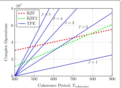
Intu-itively, precomputation is beneficial when the coherence period is long (compared toMandK), and the sequen-tial computation of TPE precoding is beneficial when the system dimensionsMandK are large (compared to the coherence period) or the coherence period is short. This is seen from the large dimensional complexity scal-ing which is O(4K2M) orO(2K2M) for RZF precoding (the latter, if the RZF or RZF2 approach is used) and O(4JKMTdatapcp) for TPE precoding; thus, the asymptotic difference is significant. The break-even point, where TPE precoding outperforms RZF, is easily computed looking at CRZFpcp >CTPEpcp
⇒Tdatapcp < 4K
2M+ K3
3 +K(M+2)−K2
4(J−1)MK+JM+(2−J)K ≈ K J−1
and similar forCpcpRZF2>CpcpTPE.
One should not forget the overhead signaling required to obtain CSI at the UTs, which makes the number of channel usesTdataavailable for data symbols reduce with
K. For example, supposeTcoherence is the total coherence
period and that we use a TDD protocol, whereηDLis the
fraction used for downlink transmission andμKchannel uses (for someμ ≥ 1) are consumed by downlink pilot signals that provide the UTs with sufficient CSI. We then have Tdata = ηDLTcoherence − μK. Using this
relation-ship, the number of arithmetic operations are illustrated numerically in Fig. 1 forηDL = 12,K = 100, andμ= 2.3
This figure shows that TPE precoding uses fewer opera-tions than RZF precoding when the coherence period is short and the TPE order is small, while RZF is competitive for long coherence times.
We remark that all previously found results change in favor of TPE, if one uses the canonical transformation of complex to real operations by doubling all dimensions.
Remark 1. Power normalization. In this section, we assumed that β and w (and ξ) are known beforehand. These factors are responsible for the power normalization of the transmit signal. Depending on the chosen normal-ization, for example, the average per one UT in this paper requires the full precoding matrix to be known. Thus, it forbids the alternative implementation of RZF precod-ing detailed before. Note that this could be remedied by changing to “strict” per UT normalization. In general, we can find values forβ andw, which only rely on channel statistics and are valid in the large(M,K) regime. This, and the possible fix for the alternative RZF approach, has motivated us to assumeβandwas known.
4.2 Delay to the first transmission for RZF and TPE
A practically important complexity metric is the num-ber of complex operations for the first channel use. This number can also be interpreted as the delay until the start of data transmission. This complexity can easily be found from the previous results, by choosing Tdata =
1. Directly looking at the massive MIMO case, we find CRZF1st = 4MK2, CRZF21st = 2MK2, and C1stTPE = 4JMK. Hence, the first data vector is transmitted by a factor of K/(2J) earlier,4 when TPE precoding is employed. This factor is significant and gives TPE precoding practical rel-evance, especially in massive MIMO systems and in very fast changing environments, i.e., when coherence peri-ods are very short. We also remark that not wasting time during the coherence period pays off greatly, as the lost channel uses are given by the saved time multiplied by the (often large) coherence bandwidth.
4.3 Implementation complexity of RZF and TPE precoding
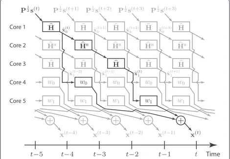
of hardware complexity, time delays, and energy con-sumption. The analysis in Subsection 4.1 showed that we can only expect improvements in the sum of complex operations from TPE precoding per coherence period in certain scenarios. However, one advantage of TPE pre-coding is that it enables multistage hardware implemen-tation where the compuimplemen-tations are pipelined [20] over multiple processing cores (e.g., application-specific inte-grated circuits (ASICs)). This structure is illustrated in Fig. 2, where the transmitted signal x(t) is prepared in various cores (black path), while the preceding and suc-ceeding transmit signals are computed in the “free” cores (gray paths). Each processing core performs two sim-ple matrix-vector multiplications, each requiring approx-imatelyO(2MK) complex additions and multiplications per coherence period. This is relatively easy to imple-ment using ASICs or FPGAs, which are know to be very energy-efficient and have low production cost. Conse-quently, we can select the TPE orderJas large as needed to obtain a certain precoding accuracy, if we are prepared to use as many circuits of the same type as needed. Then, the delay between two consecutive transmitted symbol vectors is given only by the delay of two matrix-vector multiplications.
In comparison, the inversion of RZF precoding can only be pseudo-parallelized by using tree structures. Hence, the pipelining of theCRZFcomplex operations per
coher-ence period is limited by the delay of a single process-ing core that implements the inverse of a matrix-matrix; this delay is most probably much larger than the two matrix-vector multiplications of TPE. The delay of a sec-ond core implementing the multiplication of the inverse
Fig. 2Simple pipelined implementation. A simple pipelined implementation of the proposed TPE precoding withJ=2, which removes the delays caused by precomputing the precoding matrix. Each block performs a simple matrix-vector multiplication, which enables highly efficient hardware implementation, andJcan be increased by simply adding additional cores
with the channel matrix is negligible in comparison. Like mentioned before, the precomputation of the RZF precoding matrix causes non-negligible delays that forces Tdatapcp to be smaller than for TPE precoding; for exam-ple, [35] describes a hardware implementation from [37] where it takes 0.15 ms to compute RZF precoding forK= 15, which translated to a loss of 0.15 ms × 200 kHz = 30 channel uses in a system with coherence bandwidth 200 kHz. Also, the number of active UTs can be much larger than this in large-scale MIMO systems [38]. TPE precoding does not cause such delays because there are no precomputations—the arithmetic operations are spread over the coherence period.
In practice, this means one can argue that only the curve pertaining toJ = 1 in Fig. 1 is relevant for comparisons between TPE and RZF after implementation; if one is pre-pared to add (seemingly unfairly) as many computation cores as necessary to TPE.
5 Analysis and optimization of TPE precoding In this section, we consider the large (M,K) regime, defined in Assumption 5. We show that SINRk, fork =
1,. . .,K, under TPE precoding converges to a limit, a deterministic equivalent, that depends only on the coef-ficients w, the respective attributed power pk, and the
channel statistics.
Recall the SINR expression in (5) and observe thatgk= GekandhHkGkGHkhk =hHkGG
H
hk−hHkgkgHkhk, whereekis
thekth column of the identity matrixIK. By substituting the TPE precoding expression (18) into (5), it is easy to show that the SINR writes as
SINRk = wH
Akw wHB
kw+σ2
, (19)
wherew=[w0 . . .wJ−1]Tand the(,m)th elements of the
matricesAk,Bk ∈CJ×Jare
[Ak],m=
pk Kh
H k
1 KHH
H
hkhH k
1 KHH
H
m
hk (20)
[Bk],m=
1 Kh
H k
1 KHH
H
HPH
1 KHH
H
m hk
−[Ak],m (21)
for=0,. . .,J−1 andm=0,. . .,J−1.5
Since the random matrices Ak and Bk are of finite
done by introducing the following random functionals in
Substituting (24) and (25) into (20) and (21), respec-tively, we obtain the alternative expressions
[Ak],m=
It, thus, suffices to study the asymptotic convergence of the bivariate functions Xk,M(t,u) andZk,M(t,u). This is
achieved by the following new theorem and its corollary:
Theorem 4. Consider a channel matrix H whose columns are distributed according to Assumption 3. Under the asymptotic regime described in Assumption 5, we have
Proof 2.The proof leans heavily on lemmas presented in Appendix 1 and is detailed in Appendix 2.
Corollary 1.Assume that Assumptions 1 and 5 hold true. Then, we have
Xk(,M,m)−X(M,m)−−−−−−→a.s.
Proof 3. See Appendix 4.
Corollary 1 shows that the entries ofAkandBk, which
depend on the derivatives ofXk,M(t,u)andZk,M(t,u), can
be approximated in the asymptotic regime byT()andδ(), which are the derivatives ofT(t)andδ(t)att = 0. Such derivatives can be computed numerically using the itera-tive algorithm of [21], which is provided in Appendix 6 for the sake of completeness.
It remains to compute the aforementioned derivatives. To this end, we denote f(t) = −1+t1δ(t), T(t) = −f(t)T(t), and by f(), T() their derivatives att = 0.
T()can be calculated using the Leibniz derivation rule T() = −T(t)f(t)()|t=0 = −n=0 n
T(n)f(−n) and
the respective values from Appendix 6. Rewriting (26) as
βM(t,u)
and using the Leibniz rule, we obtain for any integers andmgreater than 1, the expression
β(,m)
With these derivation results on hand, we are now in the position to determine the expressions for the deriva-tives of the quantities of interest, namely Xk,m(t,u) and
Using these results in combination with Corollary 1, we immediately obtain the asymptotic equivalents ofAkand Bk:
5.1 Optimization of the polynomial coefficients
Next, we consider the optimization of the asymptotic SINRs with respect to the polynomial coefficientsw =
[w0. . .wJ−1]T. Using results from the previous sections,
a deterministic equivalent for the SINR of thekth UT is
γk=
KpkwTAw
tr(P)wTBw+σ2.
The optimized TPE precoding should satisfy the power constraints in (8)
In order to make the optimization problem independent of the channel realizations, we replace the constraint in (28) by a deterministic one, which depends only on the
statistics of the channel. To find a deterministic equivalent of the matrixC, we introduce the random quantity
YM(t,u)=
Using the same method as for the matricesAandB, we achieve the following result:
Theorem 5.Considering the setting of Theorem 4, we have the following convergence results:
1. Letc(t,u)= K1tr(T(u)T(t))
(1+tδ(t))(1+uδ(u))(1+tuβ(t,u)), then
YM(t,u)−tr(P)c(t,u)−−−−−−→a.s. M,K→+∞ 0.
2. Denote byc(,m)theth andmth derivatives with respect tot and u, respectively, then
c(,m)=
Then, in the asymptotic regime
C−tr(P)C−−−−−−→a.s. M,K→+∞ 0.
Proof 4.The proof relies on the same techniques as before, so we provide only a sketch in Appendix 7.
Based on Theorem 5, we can consider the deterministic power constraint
tr(P)wT
Cw=P (30)
which can be seen as an approximation of (28), in the sense that for anywsatisfying (30), we have
wT
Cw−P−−−−−−→a.s.
Now, the maximization of the asymptotic SINR of UTk amounts to solving the following optimization problem:
maximize w
KpkwHAw
tr(P)wHBw+σ2
subject to tr(P)wH Cw=P.
(31)
The next theorem shows that the optimal solution,wopt,
to (31) admits a closed-form expression.
Theorem 6.Let a be a unit norm eigenvector corre-sponding to the maximum eigenvalueλmaxof
B+ σ
2
PC −1
2
A
B+σ
2
P C −1
2
. (32)
Then, the optimal value of the problem in (31) is achieved by
wopt=
P αtr(P)
B+ σ 2
P C −1
2
a, (33)
where the scaling factorαis
α= C12
B+ σ 2
P C −1
2 a
2
. (34)
Moreover, for the optimal coefficients, the asymptotic SINR for thekth UT is
γk=
Kpkλmax
tr(P) . (35)
Proof 5. The proof is given in Appendix 8.
The optimal polynomial coefficients for UTkare given in (33) of Theorem 6. Interestingly, these coefficients are independent of the user index; thus, we have indeed derived the jointly optimal coefficients. Furthermore, all users converge to the same deterministic SINR up to an UT-specific scaling factor Kpk
γtr(P).
Remark 2. The asymptotic SINR expressions in (35) are only functions of the statistics and the power allocation p1,. . .,pK. The power allocation can be optimized with
respect to some system performance metric. For example, one can show that the asymptotic average achievable rate
1 K
K
k=1
log2
1+Kpkλmax tr(P)
is maximized by a uniform power allocationpk=KP for allk.
Remark 3.Theorem 6 shows that theJpolynomial coef-ficients that jointly maximize the asymptotic SINRs can be
computed using only the channel statistics and the chan-nel estimation error. The optimal coefficients are then given in closed form in (33). Numerical experiments show that the coefficients are very robust to underestimation of τ and robust to overestimation. Hence, the main feature of Theorem 6 is that the TPE precoding coefficients can be computed beforehand or at least be updated at the rel-atively slow rate of change of the channel statistics. Thus, the cost of the optimization step is negligible with respect to calculating the precoding itself. The performance of finite-dimensional large-scale MIMO systems is evaluated numerically in Section 6.
Remark 4. Finally, we remark that Assumption 5 pre-vents us from directly analyzing the scenario whereKis fixed and M → ∞, but we can infer the behavior of TPE precoding based on previous works. In particular, it is known that MRT is an asymptotically optimal precod-ing scheme in this scenario [4]. We recall from Section 3.2 that TPE precoding reduces to MRT for J = 1. Hence, we expect the optimal coefficients to behave asw0 = 0
andw → 0 for ≥ 1 whenM → ∞. In other words, we can reduce J asMgrows large and still keep a fixed performance gap to RZF precoding.
6 Simulation results
In this section, we compare the RZF precoding from [16] (which was restated in (9)) with the proposed TPE precod-ing (defined in (18)) by means of simulations. The purpose is to validate the performance of the proposed precod-ing scheme and illustrate some of its main properties. The performance measure is the average achievable rate
r= 1 K
K
k=1
E[ log2(1+SINRk)]
of the UTs, where the expectation is taken with respect to different channel realizations and users. In the simula-tions, we model the channel covariance matrix as
[]i,j=
aj−i, i≤j,
ai−j∗, i>j,
whereais chosen to be 0.1. This approach is known as the exponential correlation model [39]. More involved models could be chosen here but would make it harder to evaluate the performance and function of TPE, while not offering more insight. The sum power constraint
tr GRZF/TPEGHRZF/TPE
=P
have setσ2= 1. Our default simulation model is a
large-scale single-cell MIMO system of dimensionsM = 128 andK=32.
We first take a look at Fig. 3. It considers a TPE order of J = 3 and three different quality levels of the CSI at the BS:τ ∈ {0.1, 0.4, 0.7}. From Fig. 3, we see that RZF and TPE achieve almost the same average UT performance when a bad channel estimate is available (τ = 0.7). Fur-thermore, TPE and RZF perform almost identically at low SNR values, for anyτ. In general, the unsurprising obser-vation is that the rate difference becomes larger at high SNRs and whenτis small (i.e., with more accurate channel knowledge).
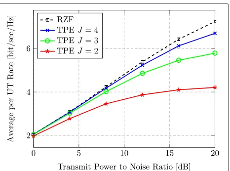
Figure 4 shows more directly the relationship between the average achievable UT rates and the TPE orderJ. We consider the caseτ =0.1,M=512, andK=128, in order to be in a regime where TPE performs relatively bad (see Fig. 3) and the precoding complexity becomes an issue. From the figure, we see that choosing a larger value forJ gives a TPE performance closer to that of RZF. However, doing so will also require more hardware; see Section 4.3. The proposed TPE precoding never surpasses the RZF performance, which is noteworthy since TPE hasJdegrees of freedom that can be optimized (see Section 5.1), while RZF only has one design parameter. Hence one can regard RZF precoding as an upper bound to TPE precoding in the single-cell scenario.6
It is desirable to select the TPE orderJ in such a way that we achieve a certain limited rate-loss with respect to RZF precoding. Figure 5 illustrates the rate-loss (per UT) between TPE and RZF, while the number of UTs K and transmit antennas M increase with a fixed ratio (M/K = 4). The figure considers the case ofτ =0.1. We observe that the TPE orderJand the system dimensions are independent in their respective effects on the rate-loss
Fig. 3Rate for varying CSI. Average per UT rate vs. transmit-power-to-noise ratio for varying CSI errors at the BS (J=3,M=128,K=32)
Fig. 4Rate for varying order. Average UT rate vs. transmit-power-to-noise ratio for different ordersJin the TPE precoding (M=512,K=128, τ=0.1)
between TPE and RZF precoding. This observation is in line with previous results on polynomial expansions, for example, [19] where reduced-rank received filtering was considered. The independence between J and the system dimensions M and K (given the same ratio) is indeed a main motivation behind TPE precoding, because it implies that the orderJcan be kept small even when TPE precoding is applied to very large-scale MIMO systems. The intuition behind this result is that the polynomial expansion approximates the inversion of each eigenvalue with the same accuracy, irrespective of the number of eigenvalues; see Section 3.2 for details. Although the relative performance loss is unaffected by the system dimensions, we also see that J needs to be increased along with the SNR, if a constant performance gap is desired.
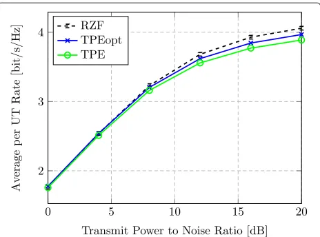
In the simulation depicted in Fig. 6, we introduce a hypothetical case of TPE precoding (TPEopt) that opti-mizes theJcoefficients using the estimated channel coef-ficients in each coherence period, instead of relying solely on the channel statistics. More precisely, the optimal coef-ficients in Theorem 6 are not computed using the deter-ministic equivalents ofA,B, andCbut using the original matrices from (20), (21), and (29). This plot illustrates the additional performance loss caused by precalculat-ing the TPE coefficients based on channel statistics and asymptotic analysis, instead of carrying out the optimiza-tion step for each channel realizaoptimiza-tion. The difference is virtually zero at low SNRs and high at high SNRs. Further-more, we note that increasing the value ofJhas the same performance-gap-reducing effect on TPEopt, as it has on TPE (see Figs. 4 and 5). In order to preserve readability, only the curves pertaining toJ=3 are shown in Fig. 6.
Finally, to assess the validity of our results, we treat the case of non-uniform power allocation (i.e., with differ-ent values forpk). In particular, we considered a situation
where the users are divided into four classes correspond-ing to{c1,c2,c4c4} = {1, 2, 3, 4}, wherepk = cKk in order
to adhere to the scaling in Assumption 4. Figure 7 shows the theoretical large (M,K) regime (DE; based on (35)) and empirical (MC; based on (19)) average rate per UT for each class, when K = 32,M = 128, andτ = 0.1. We especially remark the very good agreement between our theoretical analysis and the empirical system perfor-mance.
7 Conclusions
Conventional RZF precoding provides attractive system throughput in massive MIMO systems, but its compu-tational and implementation complexity is prohibitively
Fig. 6Rate using optimal weights. Average UT rate vs. transmit-power-to-noise ratio with RZF, TPE, and TPEopt precoding (J=3, M=128,K=32,τ=0.4)
Fig. 7Rate with power control. Average rate per UT class vs. transmit-power-to-noise ratio with TPE precoding (J=3,M=256, K=64,τ=0.1)
high, due to the required channel matrix inversion. In this paper, we have proposed a new class of TPE precoding schemes where the inversion is approximated by trun-cated polynomial expansions to enable simple hardware implementation. In the single-cell downlink withM trans-mit antennas andK single-antenna users, this new class can approximate RZF precoding to an arbitrary accuracy by choosing the TPE order J in the interval 1 ≤ J ≤ min(M,K). In terms of implementation complexity, TPE precoding has several advantages: (1) There is no need to compute the precoding matrix beforehand (which leaves more channel uses for data transmission); (2) the delay to the first transmitted symbol is reduced significantly; (3) the multistage structure enables pipelining; and (4) the parameterJcan be tailored to the available hardware.
Although the polynomial coefficients depend on the instantaneous channel realizations, we have shown that the per-user SINRs converge to deterministic values in the large (M,K) regime. This enabled us to compute asymp-totically optimal coefficients using merely the statistics of the channels. The simulations revealed that the differ-ence in performance between RZF and TPE is small at low SNRs and for large CSI errors. The TPE orderJcan be chosen very small in these situations, and in general, it does not need to scale with the system dimensions. How-ever, to maintain a fixed per-user rate-loss compared to RZF,Jshould increase with the SNR or as the CSI quality improves.
Endnotes
1Matrix multiplication combined with matrix inversion
exploit that 2×2 matrices can be multiplied efficiently and thereby reduce the asymptotic complexity of multipling/invertingK×Kmatrices toO(K2.8074)and O(K2.373), respectively. Unfortunately, the overhead in these algorithms is heavy and thusKneeds to be at the order of several thousands to achieve a lower complexity than the Cholesky approach considered here. Hence, these alternative algorithms are unfavorable for matrices of practical sizes.
2Intuitively, one circumvents the expensive
matrix-matrix multiplication with a domino-like chain of 2J−1 (less expensive) matrix-vector multiplications per transmitted symbol vector. This became possible by replacing the inverse of a matrix-matrix multiplication in the RZF with a sum of weighted matrix powers.
3These parameter values correspond to symmetric
downlink/uplink transmission, 2 downlink pilot symbols per UT (at different frequencies). Looking at values similar the LTE standard ([42] Chapter 10), e.g., a coherence bandwidth of 200 kHz, and a coherence period of 5 ms one would arrive aTcoherenceof 1000.
4Depending on the massive MIMO system,Kcan be
on the order of 100 andMof the order 10K, while we will see later thatJ=4 is sufficient for many cases.
5The entries of matrices are numbered from 0, for
notational convenience.
6The optimal precoding parametrization in [15] has
K−1 parameters. To optimize some general performance metric, it is therefore necessary to let the number of design parameters scale with the system dimensions.
Appendix 1: Useful lemmas
Lemma 2.(Common inverses of resolvents) Given any matrixH ∈ CM×K, lethk denote its kth column andHk
denote the matrix obtained after removing the kth column fromH. The resolvent matrices ofHandHkare denoted by Q(t)= KtHHH+I
M
−1
andQk(t)= KtHkHHk+IM
−1
, respectively. It then holds that
Q(t)=Qk(t)−
1 K
tQk(t)hkhHkQk(t)
1+ KthH
kQk(t)hk
(36)
and also
Q(t)hk=
Qk(t)hk
1+ KthH
kQk(t)hk
. (37)
Proof 6.This follows from the Woodbury identity [43].
The following lemma characterizes the asymptotic behavior of quadratic forms. It will be of frequent use in the computation of deterministic equivalents.
Lemma 3.(Convergence of quadratic forms) LetxM =
[X1,. . .,XM]T be a M × 1 vector with i.i.d. complex
Gaussian random variables with unit variance. Let AM
be an M×M matrix independent ofxM, whose spectral
norm is bounded; that is, there exists CA < ∞such that
A2≤CA. Then, for any p≥1, there exists a constant Cp
depending only on p, such that
ExM
M1xH
MAMxM−
1 Mtr(AM)
p ≤ CpC
p A
Mp/2,
where the expectation is taken over the distribution ofxM.
By choosing p≥2, we thus have that
1 Mx
H
AMx− 1
Mtr(AM)
a.s.
−−−−−→
M→+∞ 0.
Lemma 4.LetAM be as in Lemma 3, andxM,yM be
random, mutually independent with complex Gaussian entries of zero mean and variance 1. Then,
1 My
H
MAMxM a.s.
−−−−−−→
M,K→+∞ 0.
Lemma 5.(Rank-one perturbation lemma) LetQ(t)and
Qk(t) be the resolvent matrices as defined in Lemma 2.
Then, for any matrixAwe have
tr(A(Q(t)−Qk(t)))≤ A2.
Lemma 6.Let XMand YM be two scalar random
vari-ables, with vary such that var(XM) = O M−2
and var(XM)=O M−2
=O K−2. Then,
E[XMYM]=E[XM]E[YM]+o(1).
Proof 7.We have
E[XMYM]=
E[(XM−E[XM])(YM−E[YM])]+E[XM]E[YM] .
Using the Cauchy-Schwartz inequality, we see that
E[|(XM−E[XM]) (YM−E[YM])|]
≤var(XM)var(YM)
=O K−2
which establishes the desired result.
Appendix 2: Proof of Theorem 4
Here, we present the proof of Theorem 4, which estab-lishes the asymptotic convergence of Xk,M(t,u) and
Deterministic equivalent forXk,M(t,u)
We will begin the proof by looking at the random quantity Xk,M(t,u). Using the notation of Lemma 2, we can write
To control the quadratic form K1hH
kQ(t)hk, we need to
remove the dependency ofQ(t)on vectorhk. For that, we
shall use the relation in (36), thereby yielding
1
Using Lemma 3, we thus have
1
rank-one perturbation property in Lemma 5, we have
1
Finally, Theorem 1 implies that
1
The same kind of calculations can be used to deal with the quadratic form K1hH
between the channel estimation error and the channel vectorhk. Hence,
Plugging the deterministic approximation of (39) and (40) into (38), we thus see that
1
same steps as in section “Deterministic equivalent for Xk,M(t,u)” Appendix 2, we decomposeZk,M(t,u)as
As it will be shown next, to determine the asymptotic limit of the random variablesXi(t,u),i=1,. . ., 4, we need
to find a deterministic equivalent for
1
Ktr Q(t)HPH
H Q(u).
This is the most involved step of the proof. It will, thus, be treated separately in Appendix 3, where we establish the following lemma:
Lemma 7.Let Hbe an M×K random matrix whose columns are drawn according to Assumption 1. Define for t≥0, the resolvent matrixQ(t)= KtHHH+I
K
−1
.LetA
be an M×M deterministic matrix with uniformly spectral norm andαM(t,u,A)given as
Let us begin by treatingX1(t,u)
The right-hand side term in the equation above can be treated using (40), thereby yielding
pk
Using Lemma 3, we can prove that
1
Continuing, according to Lemma 7, we have
1
Combining (42) with (43) yields
1
Thus, in the asymptotic regime, we have
X1(t,u)− Kpk 1−τ2
difference is thatY2(t,u)is a quadratic form involving
vec-torshk andhk, whereasX1(t,u)involves only the vector hk. Following the same kind of calculations leads to
Y2(t,u)−
Finally,X4(t,u)can be treated using the same approach,
thereby providing the following convergence:
X4(t,u)−
Summing (44), (45), (46), and (47) yields
Zk,M(t,u)−
Appendix 3: Proof of Lemma 7
The aim of this section is to determine a deterministic equivalent for the random quantity
αM(t,u,A)=
1
Ktr AQ(t)HPH
H Q(u).
The proof is technical and will make frequent use of results from Appendix 1. First, we need to control var(αM(t,u)). This has already been treated in [10] where
it was proved that var(αM(t,u,A))= O(K−2)whent =
u. The same calculations hold fort=u, thus we consider in the sequel that var(αM(t,u,A))= O(K−2). Hence, we
have
αM(t,u,A)−E[αM(t,u,A)]−−−−−−→a.s.
Equation (48) allows us to focus directly on controlling
sinceZ2will be compensated by terms inZ3. We begin
withZ1:
Using Lemma 3, we can show that the first term on the right-hand side of the above equation is negligible. Therefore,
Using Lemma 5, we have
E[Z1]=
Theorem 1, thus, implies
E[Z1]=
Using (37), we arrive at
Z3= −
From (36),Z3can be decomposed as
Z3= −
We sequentially deal with the termsZ31 andZ32. The
same arguments as those used before allow us to substi-tute the denominator by 1+tδ(t), thereby yielding
By Lemma 3, the quadratic forms involved inχ2have
variance O(K−2), and thus can be substituted by their expected mean (see Lemma 6). We obtain
χ2= −t
observe that the first order of χ1 does not change if we