Volume 2008, Article ID 817876,13pages doi:10.1155/2008/817876
Research Article
Interference Aware Routing for Minimum Frame Length
Schedules in Wireless Mesh Networks
Vasilis Friderikos1and Katerina Papadaki2
1Division of Engineering, Centre for Telecommunications Research, King’s College London, Strand, London WC2R 2LS, England, UK
2Department of Management, Operational Research Group, London School of Economics, Houghton Street, London WC2A 2AE, England, UK
Correspondence should be addressed to Katerina Papadaki,[email protected]
Received 18 January 2008; Revised 4 June 2008; Accepted 15 August 2008
Recommended by Athanasios Vasilakos
The focus of this paper is on routing in wireless mesh networks (WMNs) that results in spatial TDMA (STDMA) schedules with minimum frame length. In particular, the emphasis is on spanning tree construction; and we formulate the joint routing, power control, and scheduling problem as a mixedinteger linear program (MILP). Since this is anN P-complete problem, we propose a low-complexity iterative pruning-based routing scheme that utilizes scheduling information to construct the spanning tree. A randomized version of this scheme is also discussed and numerical investigations reveal that the proposed iterative pruning algorithms outperform previously proposed routing schemes that aim to minimize the transmitted power or interference produced in the network without explicitly taking into account scheduling decisions.
Copyright © 2008 V. Friderikos and K. Papadaki. This is an open access article distributed under the Creative Commons Attribution License, which permits unrestricted use, distribution, and reproduction in any medium, provided the original work is properly cited.
1. INTRODUCTION
Algorithmic aspects of wireless mesh networks (WMNs) are currently a vigorous area of research and have steadily accumulated momentum over the last few years. The lead-ing exponents of this increased interest are the potential multifarious applications of WMNs [1]. Admittedly, the two most important of them are provision of low-cost and rapid-deployable broadband last mile connectivity to the Internet or backhaul support for 3G cells and IEEE 802.11“x” hot spots.
Efficient resource utilization in WMNs calls for schedul-ing and routschedul-ing policies that maximize the aggregate throughput of the system. Under this perspective, the central theme of this paper is the design of joint scheduling and shortest-path spanning tree schemes that provide increased system performance. With a preconstructed spanning tree within the mesh network, the cornerstone aim of the scheduling engine is either to maximize the transmission opportunities of active links in a specific time window (frame length) by taking into account the interference caused by
simultaneously transmitting nodes or to minimize the time span for all links to transmit, that is, minimize frame length. Concurrent transmissions are of utmost importance since they increase system efficiency but can lead to erroneous reception at the receiver if the level of the received signal is too weak compared to the aggregate interference. Thus, the spatial reuse of timeslots heavily depends on the selected active set of links in the mesh topology; but, the active set of links is constructed by the routing algorithm. Therefore, and as it will become vividly clear in the sequel, there is an interplay between scheduling and routing decisions. The rationale of designing joint routing and scheduling schemes stems exactly from this interplay between the two functionalities.
apart. Spatial reusing of timeslots has been defined in the seminal work of Nelson and Kleinrock [2] and is called spatial TDMA (STDMA).
In this paper, we focus on utilizing shortest-path algo-rithms, which are widely studied and used in practise. The emphasis is on Dijkstra’s algorithm which for bounded degree graphs finds the shortest paths from a source node to every other node in O(nlogn) time, where n is the number of nodes in the network. The cost metric used is the required transmission power for a link (i,j) to be established. We focus on rooted spanning tree construction (for both uplink and downlink) since the mesh mode specifications that have been integrated into the IEEE 802.16-2004 standard are based on tree topology. Our proposed pruning schemes run Dijkstra iteratively, and at each iteration, eliminate (prune) links that produce high interference; the resulting tree’s scheduling performance is evaluated by using optimal scheduling or a greedy scheduling heuristic and the tree with the best scheduling performance is kept. Thus, scheduling information is incorporated in making decisions about routing.
We compare the proposed pruning algorithm with other Dijkstra-based schemes. These heuristics use as costs linear combinations of the required power for transmission and the interference produced. We show that proposed pruning algorithm outperforms these heuristics.
The rest of the paper is organized as follows. In Section 2, selected closely related previous works in the area of joint routing and scheduling are outlined. The problem description and the mixed-integer linear program (MILP) formulation are detailed inSection 3. The inherent interplay between routing and scheduling is explained inSection 4. In Section 5, suboptimal joint scheduling and routing schemes are explained; and Section 6 outlines the two flavors of the proposed pruning algorithm. Numerical investigations are reported in Section 7; and finally, Section 8 concludes the paper by outlining the main findings followed by brief remarks on future avenues for research.
2. REVIEW OF SELECTED PRIOR WORKS
After the introduction of the spatial TDMA concept by Nelson and Kleinrock in [2], general timeslot (or channel) assignment scheduling problems have been extensively stud-ied in the literature. The bulk of previous research work focused on graph theoretic solutions by conceiving link scheduling as a graph-coloring problem [3–5]. In the basic setting, graph-coloring approaches aim to tackle theprimary
andsecondaryconflicts between links. More specifically, any
pair of directed edges (a,b), (c,d) may be colored with the same color if and only if (i) a,b,c,d are all mutually distinct and (ii) edges (a,d), (c,b) do not belong in the set of edges in the graph. When the first (second) condition fails to hold, then there will be a primary (secondary) conflict between edges (a,b) and (c,d). Scheduling based on graph theoretic tools proved essential for formally defining the problem and for the design of distributed solutions. The limitations on the other hand of these solutions stem from the fact that the aggregate effect of interference of links
transmitting in concurrent timeslots (reflected in the signal-to-interference noise ratio (SINR)) is not taken explicitly into account [6]. Hence, a schedule provided by a graph-coloring technique may lead to an infeasible allocation when the SINR thresholds are taken into account. Related to this last point is the observation that an optimal schedule based on graph coloring can be considered as a lower bound of the minimum number of timeslots that can be used in the network.
To fill this void, the authors in [7] have explicitly taken into account the SINR thresholds together with power control for constructing minimum frame length scheduling in STDMA networks with directional antennas. From a computational complexity perspective, even without taking into account the aggregate interference, constructing a trans-mission schedule of timeslots where all links are scheduled with the minimum number of timeslots (i.e., minimum frame length) has shown to be an N P-complete problem [8].
The work of Tassiulas and Ephremides [9] showed that the capacity region of wireless multihop networks depends on the power allocation vector (which itself depends on channel conditions) as well as the routing and scheduling decisions. This formal characterization of the inherent coupling between power control, scheduling, and routing, sparked a research interest in schemes that attempt to optimize them jointly [10,11]. These so-called cross-layer
optimization approaches have recently been extended to
take into account end-to-end flow and congestion control decisions (transport layer) [12]. Polynomial complexity algorithms together with necessary and sufficient conditions for optimal scheduling and routing of a predefined set of source-destination rates in mesh networks have been discussed in [13]. In contrast to these previous works, the emphasis in this paper is on how to construct spanning trees that minimize the frame length (in terms of required timeslots) in the mesh network.
Finally, it is worth mentioning that pruning techniques have been mainly used within quality of service (QoS) routing to produce a sparser graph, consisting entirely of feasible links [14,15]. In these QoS routing schemes, links are deleted from the topology if their available resources do not meet the corresponding constraints. In our case, the incentive for link pruning is a rather different one; pruning is used to delete links that produce high interference to neighbor nodes that can lead to low-spatial reuse of timeslots.
2.1. Contribution of the paper
To the authors best knowledge, this is the first paper that
explicitly addresses the issue of how to jointly construct a
spanning tree while minimizing the required frame length (in terms of the number of timeslots) in a wireless mesh network. In that respect, the contributions of the paper represent measurable progress on the following fronts:
(2) interference aware iterative pruning routing algo-rithms to construct spanning trees in the WMN with a minimum frame length schedule;
(3) quantification of the gains in terms of scheduling of the pruning schemes compared to previously proposed schemes based on an extensive set of simulations.
It is worth mentioning that even though in this paper we have assumed omnidirectional antennas (0 dB gain) and baseline path loss models, the proposed scheme is independent of the operational characteristics and models used. Thus, results drawn in this paper can be applied for different antenna radiation patterns and/or link gain models.
3. PROBLEM DESCRIPTION
Before embarking our study of suboptimal solutions in later sections, we first formulate the problem of joint routing and scheduling as an MILP.Section 3.1deals with the mathematical programming formulation for performing STDMA scheduling under the assumption of a predefined route and Section 3.2 augments the scheduling model to incorporate routing decisions.
For performing joint scheduling and routing in WMNs, we consider the graphG, defined by the (V,L) pair, where
V is a set of vertices (wireless nodes) and L is the set of transmission links that satisfy the SINR threshold criterion,
L=(u,v)|u,v∈V s.t.u /=vcan transmit tov
and vice versa. (1)
Routing is usually performed using a weighting function
w:L→R, which assigns a weight to each edge. The weight of an edge is commonly related with the required transmission power, which depends on the Euclidean distance between the nodes and the level of interference. A number of different possible edge weights that implicitly take into account scheduling information for suboptimal routing and scheduling will be discussed in the following sections.
3.1. A mixed-integer linear programming (MILP) formulation for scheduling
We first focus our attention on how to perform optimal scheduling decisions under the assumption that routing paths are preconstructed. Similar formulations appear in [16, 17]. In this case, the routing will create the directed graphGS = (V,LS), whereLS ⊆ L, and scheduling will be
performed onGS.
We encapsulate power control within the MILP formu-lation by introducing the variable pi jt, which expresses the
transmitted power by node i in link (i,j) at timeslot t, under the constraint that 0 ≤ pi jt ≤ Pmax for allt. The variablePmaxexpresses the power ceiling at the transmitting node (without loss of generalityPmaxis assumed to be equal for all nodes in the WMN). Additionally, we assume that omnidirectional antennas are used by all wireless nodes to transmit and receive signals. Thus, the interference level
produced by link (i,j) to all other receiving nodes will be based on their Euclidean distance with node i. With a constant target bit error rate (i.e., Eb/N0 = Γ), the transmission can be translated into a signal-to-interference ratio requirement, which will be denoted hereafter asγ. By
Wwe denote the lump sum thermal noise power, and bygi j
the link gain between nodesi,jwhich encapsulates both path loss and slow fading.
To be able to express now the problem in a mathematical programming setting, we introduce the boolean variablesxi jt
andπt, which are defined as follows:
xi jt=
⎧ ⎨ ⎩
1, if link (i,j) active at timeslott,
0, otherwise,
πt=
⎧ ⎨ ⎩
1, if timeslottis used,
0, otherwise.
(2)
The mixed-integer linear program for scheduling that mini-mizes the required frame length in a predefined route on the set of linksLS is denoted as OS (LS) and can be written as
follows:
min
M
t=1
πt, (3)
(i,j)∈LS
xi jt≤πt·|LS| ∀t, (4)
M
t=1
xi jt≥1 ∀(i,j)∈LS, (5)
j:(i,j)∈LS xi jt+
k:(k,i)∈LS
xkit≤1 ∀i∈V, ∀t, (6)
gi jpi jt+
1−xi jt Λ
(m,n)∈LS\{(i,j)}gm jpmnt+W ≥γ ∀(i
,j)∈LS, ∀t, (7)
xi jt≤ pi jtgi j
Wγ ∀(i,j)∈LS, ∀t, (8)
xi jt≥pi jt/Pmax ∀(i,j)∈LS, ∀t, (9)
xi jt∈ {0, 1} ∀(i,j)∈LS, ∀t, (10)
πt∈ {0, 1} ∀t, (11)
0≤pi jt≤Pmax ∀(i,j)∈LS, ∀t. (12)
In this formulation, an initial frame lengthMis assumed, where all links can be easily scheduled. For example, an initial frame length valueMcould be the number of links.
Constraints (4) are the binding constraints for variables
πt andxi jt. The requirement that all links transmit at least
once during the frame length is ensured by constraint (5). Constraint (6) is the degree constraint, that is, a node cannot transmit and receive at the same timeslot. Constraint (7) expresses the required SINR threshold that should be satisfied in order to have a successful reception at the receiver. The termΛ(1−xi jt) ensures that the inequality is
variablesxi jtandpi jtare shown in (8) and (9). These binding
constraints ensure that if link (i,j) is not transmitting at timeslott, then the transmitted power pi jt is zero and vice
versa. Constraint (8) is based on the assumption that all links (i,j) inLSsatisfy the SINR constraint when there are
no concurrent transmissions, which is equivalent togi jpi jt> γW.
3.2. Performing joint scheduling and routing
In the previous section, we formulated the scheduling problem given a fixed routing LS. Allowing flexibility with
routing decisions can improve the resulting scheduling. The aim here is to construct a routing such that the number of timeslots in a time frame is minimized. We focus our routing decisions on constructing spanning trees. The direction of the spanning tree depends on whether we are performing uplink or downlink transmission.
We augment the previously defined scheduling model to incorporate both routing (tree construction) and scheduling decisions. Note that the optimal joint routing and scheduling problem operate on the graphG=(V,L). Before describing the new constraints that need to be added, we first introduce the routing variablesyi,j, which are defined as follows:
yi j=
⎧ ⎨ ⎩
1, link (i,j) in optimal spanning tree,
0, otherwise. (13)
Without loss of generality, we assume that noderis the root node in the constructed spanning tree. Based on the above definitions, the optimal joint scheduling and spanning tree construction problem will be denoted as OSR (L), which is based on the set of all feasible links L. The mathematical formulation of the OSR (L) can be constructed by adding the following routing constraints to the already defined OS (L) formulation:
yi j≤ M
t=1
xi jt≤yi j·M ∀(i,j)∈L, (14)
(i,j)∈L:i,j∈D
yi j≤ |D| −1 ∀D⊆V, (15)
(i,j)∈L
yi j= |V| −1 ∀(i,j)∈L, (16)
j∈V:(i,j)∈L
yi j=1 ∀i∈V\ {r},
(r,i)∈L
yri=0, (17)
yi j+yji≤1 ∀(i,j)∈L. (18)
Constraint (14) binds the boolean variablesxi jt andyi j
so that a link (i,j) transmits if and only if it belongs to the optimal spanning tree. Constraint (15) ensure that there are no cycles and constraint (16) ensure that there are|V| −1 links. Since an acyclic graph with|V|nodes and|V|−1 edges is a spanning tree, the previous two constraints construct a spanning tree. Constraints (17), (18) ensure that the tree is directed in the uplink direction towards root noder. In
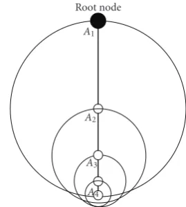
A1
A2
A3
A4 Root node
Figure 1: Worst-case scenario for timeslot reuse: the number of required timeslots is equal to the number of edges (i.e.,M= |L|).
the case of downlink, constraint (17) are replaced by the following:
j∈V:(j,i)∈L
yji=1 ∀i∈V\ {r},
(i,r)∈L
yir=0. (19)
The OSR (L) formulation constructs a tree that produces schedules with the minimal timeslot frame length. Given that OR (LS) is an N P-complete problem [8], the N P
-completeness of OSR (L) follows.
4. THE BINDING NATURE OF SPANNING TREE CONSTRUCTION AND SCHEDULING
The aim of this section is twofold. Firstly, to reveal the closely coupled nature of the spanning tree construction and the scheduling problem by focusing on the uplink transmission problem. Secondly, this discussion will motivate the pro-posed scheme with polynomial computational complexity for spanning tree construction.
Figure 1shows the worst-case scenario of a minimum power spanning tree in terms of utilization of the timeslots. As shown in the figure, the transmission areas of the nodes are nested in the sense that each node’s transmission area includes all nodes that are further away from the root node. If we define the transmission area of nodeiasAi, then nodes
{i,i+ 1,i+ 2. . .} fall within the areaAi. This means that
each nodeicannot transmit at the same timeslot as nodes
m 1 2 1 2 1 2 1 2 n Root node
Interference produced by nodemat timeslot 1 Interference produced by nodenat timeslot 2
Figure2: Best-case scenario for timeslot reuse: the number of required timeslots is equal to two.
interference produced by the nodes transmitting at timeslot one or two produce a violation on the SINR threshold.
In reality, we expect that wireless mesh network topolo-gies will lie somewhere in between the worst- and best-case scenarios described above, therefore, efficient algorithms that can provide high spatial reuse of timeslots become crucially important.
5. SHORTEST-PATH TREE CONSTRUCTION SCHEMES IN WMN’S
The joint routing and scheduling problem defined in Section 5isN P-complete and thus intractable for realistic network sizes. Thus, we turn our attention to existing routing algorithms and try to incorporate scheduling information into routing decisions.
In most widely used routing protocols for constructing trees, the paths are computed based on Dijkstra’s algorithm to find shortest-path spanning trees. The weight assigned to each link (i,j),w(i,j) is usually taken to be proportional to the power needed to transmit on link (i,j). In the sequel, we propose Dijkstra-based routing schemes that use different weights with the aim of improving link scheduling. In Section 7, we evaluate the performance of these schemes and compare them to the proposed interference aware pruning
routing scheme, described inSection 6.
5.1. Minimum power routing (MPR)
This scheme constructs shortest-path spanning trees inG= (V,L) from the root noderto all other nodesV\ {r}using Dijkstra with transmitted power as a link cost. This cost results in reduction of the overall interference. Given that the transmitted power for link (i,j) relates to the distance between nodesiand j,d(i,j), we define the following cost for MPR:
wP(i,j)=d(i,j)α, (20)
where αis the path loss exponent which varies between 2 and 4.
In order to examine the effect of Dijkstra-based routing schemes on scheduling decisions, we assume in this section
the following simple interference model: the interference caused during the transmission of link (i,j) only results in unsuccessful reception of nodes that lie within the disc with centeriand radiusd(i,j). Any receiving nodes that lie outside the disc are unaffected. We call this model as disc-based interference (it is also widely known as the protocol
interference model[18]).
Proposition 1. Assuming a disc-based interference model, the
MPR scheme does not result in a schedule with minimum timeslot frame length.
Proof. We show this using a counter example. Figure 3(a)
shows the shortest-path spanning tree constructed by MPR for the given topology in the case of downlink transmission. In the MPR tree, the transmission of link (i,m) is affecting
five links (including the link that has a degree constraint with link (i,m)). These five links require four timeslots (minimum), and since none of them can be reused, the required number of timeslots should be increased by one to accommodate link (i,m). In the tree shown in Figure3(b), nodemis connected via node j. In this case, the link (j,m) is affecting two links (the link from root node to noden, and link (n,j)), and, therefore, one of the four timeslots from the other branch of the tree can be reused.
The tree depicted inFigure 3(b) is not a shortest-path spanning tree with respect towP since the path from node m to the root node is longer than the equivalent path in Figure 3(a). However, the tree in Figure 3(b) produces a schedule with shorter frame length (in terms of times-lots).
Shortest-path spanning trees can be computed in poly-nomial time using the Dijkstra or Bellman-Ford algorithms. A brute force approach to find the tree with the minimum frame length would be to enumerate all possible trees and for each one to perform optimal scheduling. Even without taking into account the embedded scheduling problem, enu-merating all trees has exponential computational complexity due toProposition 2.
Proposition 2 (Cayleys Formula). The number of labeled
1
2 3
2
4 2
5
3 n
j
m i
d1 Root node
(a)
1 2
3 2
4 2
3
4 n
j
m i
d2 Root node
(b)
Figure3: (a) Minimum power spanning tree (MPST), and (b) a spanning tree that requires less number of timeslots (better spatial reuse). Timeslots are shown within the rectangular boxes.
5.2. Minimum nearest neighborhoods routing—MNR
The MNR algorithm tries to minimize the number of nodes that are within the area of each link in the shortest-path spanning tree. In order to compute such a tree, Dijkstra’s algorithm can be deployed where the cost of each link (i,j)∈
Lis equal to the number of receiving nodes that are within its transmission range (taken to be the disc of centeriand radius
d(i,j)). In this case, the cost can be written as follows:
wN(i,j)=
n∈V\{i,j,r}
I(i,j)(n), (21)
whereI(i,j)(n) is the indicator function which is defined as
follows forn /=i,j:
I(i,j)(n)=
⎧ ⎨ ⎩
1, ifd(i,n)≤d(i,j),
0, otherwise. (22)
This algorithm can also include a lower bound on the number of nodes that are within the transmission range of each link so that connectivity can be established with high probability [19].
a
b
c
d
Figure4: Possible edge crossing in the minimum nearest neighbor-hoods spanning tree algorithm.
A drawback of this scheme is that it may introduce edge crossings in the constructed tree.
Proposition 3. The MNR scheme may create shortest-path
spanning trees that are nonplanar graphs.
Proof. Figure 4shows a possible construction of a spanning
tree based on the MNR algorithm. The root node is nodea
and after the construction of links (a,b), which has cost 0, and (a,c), which has cost 1, the cost of the link (b,d) is 4 (nodes within the circle shown by solid lines) whilst the cost for links (a,d) and (c,d) is 5 and 7, respectively (nodes within the dashed and doted dashed circles, resp.). Thus, the least-cost path to nodedis through nodeband, therefore, an edge crossing will be introduced.
Link crossing can be detected, and, subsequently, pla-narity can be restored, but the current proposed techniques need to be adapted before being applied for tree construction (see [20] and references therein).
5.3. Interference based routing—IR
In this case, the actual interference that will be produced to the other receiving nodes in the network is taken into account to produce the cost for every link in the network. More specifically, the cost for link (i,j) is computed as follows:
wI(i,j)=
n∈V\{i,j,r}g(i,n)
g(i,j) . (23)
Therefore, the cost for link (i,j) is inversely proportional to the link gaing(i,j) but weighted with the aggregate link gains of nodeito all other receiving nodes in the network. Thus, the actual interference that will be produced by link (i,j) is explicitly taken into account.
5.4. Weighted power and interference routing (WPIR)
condensed into a single metric via a linear combination. The cost for link (i,j) can be, therefore, written as follows:
wPI(i,j)=βwP(i,j)Θ+ (1−β)wI(i,j), (24)
where β controls the weight of each individual metric in the cost and Θ is a normalizing constant between the average wP and wI values. By this linear combination, a
single weight is assigned to every link and thus it becomes possible to use a Dijkstra-like algorithm. Since different spanning trees will be constructed with different values ofβ, a drawback of this scheme is that by linearly combining the two metrics, the optimal weighting value will be different for different topologies. This routing scheme is similar to the one discussed in [21].
6. INTERFERENCE AWARE PRUNING ROUTING ALGORITHM—IAPR
The algorithm presented herein is based on an iterative version of the Dijkstra’s shortest-path algorithm. At each iteration of the algorithm, links that produce the highest interference are pruned in later iterations of the algorithm. The idea is that by excluding links that produce severe interference, the spatial timeslot reuse could be enhanced.
At iteration k, a shortest-path spanning tree Tk is
constructed using weights wP based on the set of available
links, and scheduling is performed on Tk to find the
minimum frame lengthSk to schedule all links in the tree.
The functionIk(e) is a metric of interference produced by
linkeat iteration kin shortest-path spanning treeTk. The
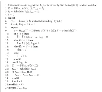
spanning tree is updated at each iteration by removing the link with the highest interference and running Dijkstra on the remaining links. We keep the spanning that produced a schedule with the minimum frame length. This continues until the stopping criteria of the algorithm are satisfied. The pseudocode of the proposed IAPR scheme is shown in Algorithm 1.
6.1. Properties of the IAPR scheme
Since the pruning algorithm eliminates at each iteration links that have been previously used in constructing shortest-path spanning trees, the aggregate shortest-shortest-path cost will not decrease with iterations. This characteristic of the IAPR scheme is encapsulated in the following result. Let us denote bypk(i) the aggregate power for the shortest path inTkfrom
the root node to node i(downlink case), and letK be the maximum number of iterations that the pruning scheme runs.
Proposition 4. If by Pk =
i∈V\{r}pk(i) we denote the
aggregate transmitted power in tree Tk constructed by IAPR
algorithm at iterationsk, then
P1≤P2≤ · · · ≤PK. (25)
The result below is specific to the downlink case, however, the corresponding result for the uplink holds.
1:G(V,L)←G(V,L), pre-processing (seeSection 6.2) 2:k←0,
3:K, maximum number of iterations 4:T, best spanning tree found so far 5:S, minimum frame length achieved so far 6:Tk←∅, spanning tree at iterationk
7:Sk= |L|, frame length achieved at iterationkby treeTk
8:repeat
9: ifk=0then
10: Tk+1←Dijkstra usingwPonG(V,L)
11: else
12: Tk+1←Modified Dijkstra usingwPonG(V,L)
13: end if
14: Sk+1←Schedule(Tk+1) 15: ifSk+1< Sthen 16: T←Tk+1 17: S←Sk+1 18: end if
19: Find linke∈Lsuch thatIk+1(e)=maxl∈L{Ik+1(l)} 20: L←L\ {e}
21: k←k+ 1 22:until(k > K) 23:returnT,S
Algorithm1: Interference aware pruning routing (IAPR).
Lemma 1. Suppose link(i,j) is eliminated at iterationk of the IAPR algorithm in the downlink case. Then, there exists at
least one spanning tree found at iterationk+ 1,Tk+1with the
following property: all nodes of treeTk, that nodejis not one of
their parents, will have the same predecessor in treeTk+1.
Proof. Since link (i,j)∈Tk, (i,j) belongs to the shortest path
from root node to nodejinTk. Eliminating (i,j) at iteration k, the shortest-path cost to node j inTk+1will increase (or remain the same). Thus, pk+1(j) ≥ pk(j). Thus, any node
that did not have node jas a parent in treeTkwill not havej
as a parent in treeTk+1.
Lemma 1indicates that trees Tk and Tk+1 may have a large set of common links. This observation motivates the following modification of the Dijkstra algorithm.
Definition 1. Themodified Dijkstraalgorithm takes as input
the graphGk =(V,Lk), the shortest-path spanning treeTk
ofGk, and a link (i,j)∈Tk,Lk, and produces a spanning tree Tk+1ofGk+1=(V,Lk+1), whereLk+1=Lk\ {(i,j)}.
(1) The set of nodes V is partitioned into two sets:V1 is the set of nodes whose shortest path from the root node onTkincludes link (i,j), andV2is the set of all remaining nodes.
(2) The modified Dijkstra assumes that shortest paths for nodes inV2are the same as the ones constructed in treeTk. Thus, shortest paths for this set of nodes are
not recalculated.
Proposition 5. The tree produced by the modified Dijkstra algorithm is a shortest-path spanning tree.
Proof. The proof follows fromLemma 1.
The above modification of the Dijkstra algorithm is used to accelerate the updating of trees in the IAPR scheme at iterationsk≥1.
6.2. Preprocessing on the initial graph
In order to accelerate the performance of the algorithm, the following preprocessing step can be implemented. In graph
G(V,L) of WMN, the setLof links is reduced by considering only links (i,j) that havewN(i,j)≤Nmax(i.e., only links with less thanNmaxneighbors are considered) (seeSection 5.2).
6.3. Complexity of IAPR
The computational complexity that pertains one iteration of the algorithm is that of the modified Dijkstra algorithm, the pruning operation, and the scheduling engine. Assuming a greedy packing heuristic for scheduling (see Section 7), the complexity of each aforementioned step in one iteration is O(nlogn). In the worst-case scenario, the algorithm terminates after K iterations, thus the complexity of the overall computational can beO(Knlogn) steps.
6.4. Stopping criterion
In general, a stopping criterion is needed to avoid pruning links that are required to ensure connectivity. A possible stopping criterion could be to hault the algorithm at the iteration at which the remaining links no longer can ensure a connected graph. This would mean that we run the algorithm in the order of|V|2iterations, in the case of dense networks, that is, complete graphs. However, in practise after the removal of a few high interference links at the beginning, the algorithm will stop improving. Even though the algorithm will not deteriorate after many iterations (since we keep the best schedule), it will be unnecessary to run it until the graph is disconnected. This is intuitive and we have also verified it experimentally as will be shown in later sections. Thus, either a relatively small number of iterations should be chosen or the algorithm should run within some predefined small time limit. An operator, for example, can put a maximum time limit on the computational time for running the routing algorithm. In that case, the number of iterations will be limited by this time limit.
6.5. A randomized version of the IAPR
At each iteration of the IAPR scheme, the link that produces the highest interference is pruned with probability one, irrespectively of whether the framelength is decreased or not. A variation of the scheme could be to check a number of links ordered by the level of interference they produce, and prune the first link whose removal improves the framelength. In this case, a number of pruning options are considered
and the scheme proceeds in the direction that improves the framelength. However, in the case that none of the V −1 links of the shortest-path tree (when pruned) improve the framelength, the above scheme will be unable to search further and thus stall. In order to further increase the search space and at the same time avoid stalling, we randomize the above scheme by pruning a link with a small probability
p, even though the resulting frame length produced by removing this link is not leading to an improvement. The pseudocode of the randomized version of the IAPR scheme (R-IAPR) is shown in Algorithm 2. In the worst-case scenario, the algorithm in each iteration will test all links in the shortest-path tree. Therefore, the computational complexity of the R-IAPR scheme can beO(K(V−1)nlogn) steps.
7. NUMERICAL INVESTIGATIONS
In this section, we evaluate the performance of the proposed IAPR scheme (both the deterministic and randomized one) compared to the MPR, MNR, IR, and WPIR schemes that have been detailed in Section 5. Simulations are con-ducted on different randomly generated WMN topolo-gies. For all different schemes, a simple greedy heuristic for evaluating the scheduling has been used, which is described inAlgorithm 3. We denote bySthe frame length achieved by either the optimal scheduling or the packing heuristic.
The packing heuristic tries to pack as many links as
possible in each time slot that have not yet transmitted in previous time slots (listA), giving priority to the ones with the highest transmitted power. This continues until all links have transmitted at least once (listAis empty). Thispacking
heuristicis similar to a heuristic used in [16,22,23], where it
was shown to produce satisfactory solutions.
The IAPR (and R-IAPR) scheme uses the packing heuristic at each iteration to evaluate the scheduling of the current shortest path spanning tree. Further, we use the following function to evaluate the interference caused by each link (i,j) in the shortest-path spanning tree Tk: Ik((i,j)) = wN(i,j), that is, the number of receiving nodes
that are within the disc with centeriand radiusd(i,j). For the WPIR scheme, the value ofΘhas been selected to normalize the average power weightwP and the average
interference weight wI. The value ofβ = 0.5, which gives
equal weight to the two metrics, has been used in the simulations.
For the numerical investigations reported in the fol-lowing sections the parameterization of the simulation environment is as follows. The path loss model for link (i,j) is PLd(i,j) = PL (do) + 10ηlog10(d(i,j)/do), where d(i,j)
is the distance of link (i,j), PL (do) is the close in distance
loss (40 dB) for distancedo (100 m), andηis the path loss
exponent, which is assumed to be equal to 3. The value of the SINR thresholdγis 5 dB. The thermal and background noise at the receiverW is assumed to be 10−11 Watt, the carrier frequency 2500 MHz, and the maximum transmission power
1: Initialization as inAlgorithm 1,p,r(uniformly distributed [0, 1] random variable) 2:T0←DijkstraG(V,L);Tbest←T0
3:S0←Schedule(T0);Sbest←S0 4:k←0
5:repeat
6: Hk+1←Links inTksorted (descending) byIk(·)
7: S←Sk; flag←1;i←1
8: repeat
9: e←Hk+1;T ←DijkstraG(V,L\ {e});S ←Schedule(T) 10: ifS < Sthen
11: L←L\ {e};S←S; flag←0 12: else ifr < pthen
13: L←L\ {e}; flag←0 14: else ifi=V−1then 15: flag←0
16: else 17: i←i+ 1; 18: end if 19: untilflag=0
20: Tk+1←DijkstraG(V,L) 21: Sk+1←Schedule(Tk+1) 22: ifSk+1< Sbestthen 23: Sbest←Sk+1;Tbest←Tk+1 24: end if
25: k←k+ 1 26:until(k > K) 27:returnTbest,Sbest
Algorithm2: Randomized interference aware pruning routing (R-IAPR).
Note: The packing heuristic does not perform power control and assumes that each link transmits with power that is 10% higher than the minimum power needed to transmit on its own, i.e., when there is no interference.
1: LetAbe a list of all links sorted according to transmitted power (highest power first). Let Bbe an empty list andt=1. At timeslottschedule the first link in listAfor transmission and shift it from listAto listB
2:repeat
3: Proceed down the current listAscheduling links for transmission in timeslott, if feasible, and shifting them to listBif they transmit
4: Lett←t+ 1 5:untilAis empty 6:returnt−1
Algorithm3: Packing heuristic.
7.1. Main results
The performance of the different routing schemes has been tested with varying number of nodes in the WMN. The average frame length (in terms of timeslots) and the standard deviation of the framelength has been measured for 100 random uniformly distributed WMN’s with 40, 60, and 80 nodes. The packing heuristic was used to evaluate the scheduling and the results are detailed in Table 1. From Table 1, two interesting conclusions can be drawn. The first one is that in all different scenarios, the IAPR scheme
11 10 9 8 7 6 5 4 3 2 1 0
Ti
m
es
lo
ts
(a) (b) (c) (d) (e)
11 10 9 8 7 6 5 4 3 2 1 0
Ti
m
es
lo
ts
(a) (b) (c) (d) (e)
Figure5: Required number of timeslots for optimal scheduling in the case of top 60 nodes and bottom 40 nodes: (a) minimum power routing (MPR), (b) interference aware pruning routing (IAPR), (c) minimum neighbors routing (MNR), (d) interference routing (IR), and (e) weighted power and interference routing (WPIR).
Table1: Performance of the routing schemes in WMN topologies with varying number of nodes.
Nodes 40 60 80
Timeslots avg. std avg. std avg. std MPR 18.70 1.98 22.33 1.81 24.07 1.71 IAPR 18.10 1.97 21.27 1.57 23.10 1.37 MNR 20.27 1.95 23.8 1.86 26.63 1.63 IR 20.10 1.58 23.6 1.81 26.2 1.84 WPIR 18.93 1.78 22.43 1.55 24.26 1.82
inherent difficulties of tuning theβ,Θvalues for the WPIR so that it can outperform the MPR.
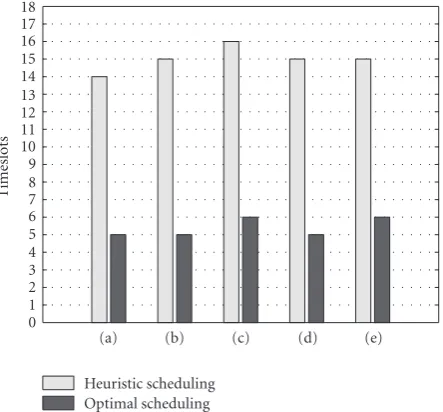
For the same random topologies of 40 and 60 nodes, we test the performance of the different routing schemes using optimal scheduling and the results are shown in Figure 5. When using the optimal scheduling, the average frame length for all different routing schemes is approximately the same (except for MNR and IR schemes which require slightly larger frame lengths). In other words, an optimal scheduling
18 17 16 15 14 13 12 11 10 9 8 7 6 5 4 3 2 1 0
Ti
m
es
lo
ts
(a) (b) (c) (d) (e)
Heuristic scheduling Optimal scheduling
Figure 6: Comparison between packing heuristic and optimal scheduling for the different routing schemes for the case of 18 nodes: (a) interference aware pruning routing (IAPR), (b) minimum power routing (MPR), (c) minimum neighbors-based routing (MNR), (d) interference routing (IR), and (e) weighted power and interference routing (WPIR).
1 0.9 0.8 0.7 0.6 0.5 0.4 0.3 0.2 0.1 0
F
(
x
)
5 10 15 20 25
x Empirical CDF
Figure7: The empirical cumulative distribution function (cdf) of the number of pruning iterations for finding the minimum schedule in terms of timeslots.
engine can compensate the decisions from the routing engine and thus being able to successfully pack all transmission in almost the same number of timeslots irrespectively of the routing scheme. Despite this fact, the IARP scheme is still very robust to different topologies. As can be seen from the error bar, which expresses the standard deviation, in Figure 5, the std of the frame length for the IARP scheme is approximately 30% less than that of the MPR scheme.
2
with 18 nodes. For this topology, the minimum number of timeslots computed by CPLEX was 5 (this solution was found within 200 seconds). In Figure 6, we compare the number of timeslots computed for the same topology for the different routing schemes with optimal and heuristic scheduling. As can be seen from the figure, when using the heuristic scheduling, the pruning scheme provides a 6.7% improvement compared to the other routing schemes. It is also worth mentioning that when using the optimal scheduling, three out of five routing schemes achieve the same number of timeslots as the optimal joint scheduling and routing.
One interesting question is that if we run the pruning algorithm for a fixed number of iterations, at which iteration will it find the schedule with the minimum possible frame length? To shed some light on that question, we have performed the following experiment. For a specific number of nodes in the network, namely, 40 in this case, 100 uniformly distributed topologies have been generated in a 3×3 km rectangular area. For each topology, we perform 30 pruning operations and store the iteration where the IAPR scheme found the frame length with the minimum number of timeslots. We have repeated this procedure for each topology and the result is shown in Figure 7, which depicts the empirical cumulative distribution function (cdf) that has been obtained by the experiment. The empirical cdf reveals that with 90% probability, the pruning algorithm finds the schedule with the minimum timeslot span in less than 14 iterations.
7.2. Randomized pruning scheme
In Section 6.5, we described a variation of the pruning scheme (called R-IAPR) that increases the search space for a better solution by testing more links or by randomizing the search. After demonstrating the improvement performed by the IAPR scheme inSection 7.1, we proceed to demonstrate that the randomized version of the IAPR scheme can offer further improvement.
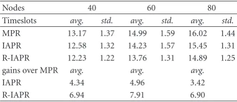
Table 2 shows the average framelength (in terms of timeslots) and the standard deviation of the frame length, averaged over 100 random uniformly distributed WMN topologies with 40, 60, and 80 nodes, respectively, for the MPR, IAPR, and R-IAPR schemes. For the R-IAPR scheme, we used pruning probabilityp=1/3V(seeSection 6.5). The average gains of the pruning schemes are also displayed. We observe that the improvement in performance is evident over all three network sizes, with the randomized pruning scheme offering a consistent enhancement in performance over the IAPR scheme.
7.3. Routing illustrations
Figure 8shows the spanning trees constructed by the differ-ent schemes in the case of a random WMN topology with 30 nodes. In this scenario, the packing heuristic has been used as the scheduling technique for evaluating the frame lengths produced by the different routing schemes. The IAPR scheme requires 17 timeslots (Figure 8(a)), while the R-IAPR
Table 2: Average timeframes of MPR, IAPR, R-IAPR routing schemes, and average performance gains of the pruning schemes.
Nodes 40 60 80
Timeslots avg. std. avg. std. avg. std. MPR 13.17 1.37 14.99 1.59 16.02 1.44 IAPR 12.58 1.32 14.23 1.57 15.45 1.31 R-IAPR 12.23 1.22 13.76 1.31 14.89 1.25 gains over MPR avg. avg. avg.
IAPR 4.34 4.96 3.42
R-IAPR 6.94 7.91 6.90
scheme requires 16 timeslots (Figure 8(b)). These should be compared to the MPR and the WPIR schemes, which both require 19 timeslots (Figures8(c) and8(b), resp.). Thus, the R-IARP scheme provides more than 15% improvement over the MPR. It is also interesting to note that for this scenario, the MNR scheme achieved the same frame length as the IARP. Note also that even though the spatial reuse for MPR, WPIR, and IR schemes is the same, the constructed spanning trees are very different.
8. CONCLUSIONS
In this paper, an interference aware pruning-based routing scheme has been proposed which strives to optimize path selection and STDMA scheduling. A randomized version of the pruning scheme has also been detailed and has been shown to improve the later heuristic. We have formu-lated the corresponding MILP to perform joint scheduling and routing, and used this formulation to compare the performance of the proposed scheme with the optimal joint scheduling and routing. The routing schemes were evaluated using both a greedy scheduling heuristic and optimal scheduling. Extensive performance evaluation in different network settings of the proposed scheme revealed that it outperforms the previously proposed routing schemes where interference and power consumption are used as a routing metric.
We should note that the general nature of the algorithms presented in this paper, including the proposed ones, is applicable to more general network settings that can include directional pattern transmissions and link gains that capture more precisely slow signal variations due to the physical terrain. Furthermore, we merely looked at the joint routing and scheduling problem without considering flows and the corresponding requirement of conserving them. This simplification allowed us to shed light into the interplay between the two engines and compare different schemes. We left the study of such augmented models that incorporate network flow requirements as an avenue of future research.
REFERENCES
[2] R. Nelson and L. Kleinrock, “Spatial TDMA: a collision-free multihop channel access protocol,”IEEE Transactions on Communications, vol. 33, no. 9, pp. 934–944, 1985.
[3] B. Hajek and G. Sasaki, “Link scheduling in polynomial time,” IEEE Transactions on Information Theory, vol. 34, no. 5, part 1, pp. 910–917, 1988.
[4] C. G. Prohazka, “Decoupling link scheduling constraints in multi-hop packet radio networks,” IEEE Transactions on Computers, vol. 38, no. 3, pp. 455–458, 1989.
[5] A.-M. Chou and V. O. K. Li, “Slot allocation strategies for TDMA protocols in multihop packet radio networks,” in Proceedings of the the 11th Annual Joint Conference of the IEEE Computer and Communications Societies (INFOCOM ’92), vol. 2, pp. 710–716, Florence, Italy, May 1992.
[6] A. Behzad and I. Rubin, “On the performance of graph-based scheduling algorithms for packet radio networks,” in Proceedings of the IEEE Global Telecommunications Conference (GLOBECOM ’03), vol. 6, pp. 3432–3436, San Francisco, Calif, USA, December 2003.
[7] A. K. Das, R. J. Marks, P. Arabshahi, and A. Gray, “Power controlled minimum frame length scheduling in TDMA wireless networks with sectored antennas,” inProceedings of the 24th Annual Joint Conference of the IEEE Computer and Communications Societies (INFOCOM ’05), vol. 3, pp. 1782– 1793, Miami, Fla, USA, March 2005.
[8] S. Even, O. Goldreich, S. Moran, and P. Tong, “On the NP-completeness of certain network testing problems,”Networks, vol. 14, no. 1, pp. 1–24, 1984.
[9] L. Tassiulas and A. Ephremides, “Stability properties of constrained queueing systems and scheduling policies for maximum throughput in multihop radio networks,” IEEE Transactions on Automatic Control, vol. 37, no. 12, pp. 1936– 1948, 1992.
[10] R. L. Cruz and A. V. Santhanam, “Optimal routing, link scheduling and power control in multihop wireless networks,” inProceedings of the 22nd Annual Joint Conference of the IEEE Computer and Communications Societies (INFOCOM ’03), vol. 1, pp. 702–711, San Francisco, Calif, USA, March-April 2003. [11] K. Kar, M. Kodialam, T. V. Lakshman, and L. Tassiulas,
“Routing for network capacity maximization in energy-constrained ad hoc networks,” in Proceedings of the 22nd Annual Joint Conference on the IEEE Computer and Commu-nications Societies (INFOCOM ’03), vol. 1, pp. 673–681, San Francisco, Calif, USA, March-April 2003.
[12] L. Chen, S. H. Low, M. Chiangs, and J. C. Doyle, “Cross-layer congestion control, routing and scheduling design in ad hoc wireless networks,” in Proceedings of the 25th IEEE International Conference on Computer Communications (INFOCOM ’06), pp. 1–13, Barcelona, Spain, April 2006. [13] M. Kodialam and T. Nandagopal, “Characterizing achievable
rates in multi-hop wireless mesh networks with orthogonal channels,”IEEE/ACM Transactions on Networking, vol. 13, no. 4, pp. 868–880, 2005.
[14] Z. Wang and J. Crowcroft, “Quality-of-service routing for supporting multimedia applications,”IEEE Journal on Selected Areas in Communications, vol. 14, no. 7, pp. 1228–1234, 1996. [15] G. Liu and K. G. Ramakrishnan, “A∗Prune: an algorithm for finding K shortest paths subject to multiple constraints,” in Proceedings of the 20th Annual Joint Conference of the IEEE Computer and Communications Societies (INFOCOM ’01), vol. 2, pp. 743–749, Anchorage, Alaska, USA, April 2001.
[16] K. Papadaki and V. Friderikos, “Approximate dynamic pro-gramming for link scheduling in wireless mesh networks,” Computers & Operations Research, vol. 35, no. 12, pp. 3848– 3859, 2008.
[17] V. Friderikos, K. Papadaki, D. Wisely, and H. Aghvami, “Multi-rate power-controlled link scheduling for mesh broadband wireless access networks,”IET Communications, vol. 1, no. 5, pp. 909–914, 2007.
[18] P. Gupta and P. R. Kumar, “The capacity of wireless networks,” IEEE Transactions on Information Theory, vol. 46, no. 2, pp. 388–404, 2000.
[19] H. Takagi and L. Kleinrock, “Optimal transmission ranges for randomly distributed packet radio terminals,”IEEE Transac-tions on CommunicaTransac-tions, vol. 32, no. 3, pp. 246–257, 1984. [20] Y.-J. Kim, R. Govindan, B. Karp, and S. Shenker,
“Geo-graphic routing made practical,” inProceedings of the USENIX Symposium on Network Systems Design and Implementation (NSDI ’05), pp. 217–230, Boston, Mass, USA, May 2005. [21] G. Heijenk and F. Liu, “Interference-based routing in
multi-hop wireless infrastructures,”Computer Communications, vol. 29, no. 13-14, pp. 2693–2701, 2006.
[22] J. Gronkvist, “Traffic controlled spatial reuse TDMA in multi-hop radio networks,” in Proceedings of the 9th IEEE International Symposium on Personal, Indoor and Mobile Radio Communications (PIMRC ’98), vol. 3, pp. 1203–1207, Boston, Mass, USA, September 1998.