How to manipulate curve standards: a white paper for the black hat

(1)

a white paper for the black hat

Daniel J. Bernstein1,2, Tung Chou1, Chitchanok Chuengsatiansup1, Andreas H¨ulsing1_{, Eran Lambooij}1_{, Tanja Lange}1_,

Ruben Niederhagen1, and Christine van Vredendaal1 1 _{Department of Mathematics and Computer Science}

Technische Universiteit Eindhoven, P.O. Box 513, 5600 MB Eindhoven, NL [email protected], [email protected],

[email protected], [email protected], [email protected], [email protected], [email protected]

2 _{Department of Computer Science}

University of Illinois at Chicago, Chicago, IL 60607–7045, USA [email protected]

Abstract. This paper analyzes the cost of breaking ECC under the following assump-tions: (1) ECC is using a standardized elliptic curve that was actually chosen by an attacker; (2) the attacker is aware of a vulnerability in some curves that are not pub-licly known to be vulnerable.

This cost includes the cost of exploiting the vulnerability, but also the initial cost of computing a curve suitable for sabotaging the standard. This initial cost depends heav-ily upon the acceptability criteria used by the public to decide whether to allow a curve as a standard, and (in most cases) also upon the chance of a curve being vulnerable.

This paper shows the importance of accurately modeling the actual acceptability cri-teria: i.e., figuring out what the public can be fooled into accepting. For example, this paper shows that plausible models of the “Brainpool acceptability criteria” allow the attacker to target a one-in-a-million vulnerability and that plausible models of the “Microsoft NUMS criteria” allow the attacker to target a one-in-a-hundred-thousand vulnerability.

Keywords. Elliptic-curve cryptography, verifiably random curves, verifiably pseu-dorandom curves, minimal curves, nothing-up-my-sleeve numbers, ANSI X9, NIST, SECG, Brainpool, Microsoft NUMS, sabotaging standards, fighting terrorism, protect-ing the children.

(2)

1 Introduction

More and more Internet traffic is encrypted. This poses a threat to our society as it limits the ability of government agencies to monitor Internet communication for the prevention of terrorism and globalized crime. For example, an increasing number of servers use Transport Layer Security (TLS) as default (not only for transmissions that contain passwords or payment information) and also most modern chat applications encrypt all communication. This increases the cost of protecting society as it becomes necessary to collect the required information at the end points, i.e., either the servers or the clients. This requires agencies to either convince the service providers to make the demanded information available or to deploy a back door on the client system respectively. Both actions are much more expensive for the agencies than collecting unprotected information from the transmission wire.

Fortunately, under reasonable assumptions, it is feasible for agencies to fool users into deploying cryptographic systems that the users believe are secure but that the agencies are able to break.

1.1. Elliptic-curve cryptography. Elliptic-curve cryptography (ECC) has a reputation for high security and has become increasingly popular. For definite-ness we consider the elliptic-curve Diffie–Hellman (ECDH) key-exchange proto-col, specifically “ephemeral ECDH”, which has a reputation of being the best way to achieve forward secrecy. The literature models ephemeral ECDH as the following protocol ECDHE,P, Diffie–Hellman key exchange using a point P on an elliptic curveE:

1. Alice generates a private integera and sends the ath multiple of P on E. 2. Bob generates a private integer b and sends bP.

3. Alice computes abP as the ath multiple ofbP. 4. Bob computes abP as the bth multiple of aP.

5. Alice and Bob encrypt data using a secret key derived from abP.

There are various published attacks showing that this protocol is breakable for many elliptic curvesE, no matter how strong the encryption is. See Section2for details. However, there are also many (E, P) for which the public literature does not indicate any security problems. Similar comments apply to, e.g., elliptic-curve signatures.

This model begs the question of where the curve (E, P) comes from. The standard answer is that a central authority generates a curve for the public (while advertising the resulting benefits for security and performance).3 This does not mean that the public will accept arbitrary curves; our main objective in this paper is to analyze the security consequences of various possibilities for 3 _{See, e.g., ANSI X9.62 [}₁_{] (“public key cryptography for the financial services}

(3)

what the public will accept. The general picture is that Alice, Bob, and the central authority Jerry are actually participating in the following three-party protocol ECDHA, where A is a function determining the public acceptability of a standard curve:

−1. Jerry generates a curveE, a pointP, auxiliary dataSwithA(E, P, S) = 1. (The “seeds” for the NIST curves are examples ofS; see Section4.) 0. Alice and Bob verify that A(E, P, S) = 1.

1. Alice generates a private integer a and sends aP. 2. Bob generates a private integer b and sends bP. 3. Alice computes abP as the ath multiple ofbP. 4. Bob computes abP as the bth multiple of aP.

5. Alice and Bob encrypt data using a secret key derived from abP.

Our paper is targeted at Jerry. We make the natural assumption that Jerry is cooperating with a heroic eavesdropper Eve to break the encryption used by potential terrorists Alice and Bob. The central question is how Jerry can use his curve-selection flexibility to minimize the attack cost.

Obviously the costcAof breaking ECDHA depends onA, the same way that the cost cE,P of breaking ECDHE,P depends on (E, P). One might think that, to evaluate cA, one simply has to check what the public literature says about cE,P, and then minimize cE,P over all (E, P, S) with A(E, P, S) = 1. The reality is more complicated, for three reasons:

1. There may be vulnerabilities not known to the public: curves E for which cE,P is smaller than indicated by the best public attacks. Our starting assumption is that Jerry and Eve are secretly aware of a vulnerability that applies to a fraction of all curves that the public believes to be secure. The obvious strategy for Jerry is to standardize a vulnerable curve. Of course, Jerry should object to any public suggestions that a vulnerable curve could have been standardized.

2. Some choices of A limit the number of curves E for which there exists suitable auxiliary data S. If 1/ is much larger than this limit then Jerry cannot expect any vulnerable (E, P, S) to haveA(E, P, S) = 1. We show that, fortunately for Jerry, this limit is much larger than the public thinks it is. See Sections 5 and6.

3. Other choices of A do not limit the number of vulnerable E for which S exists but nevertheless complicate Jerry’s task of finding a vulnerable (E, P, S) withA(E, P, S) = 1. See Section4for analysis of the cost of this computation.

If Jerry succeeds in finding a vulnerable (E, P, S) withA(E, P, S) = 1, then Eve simply exploits the vulnerability, obtaining access to the information that Alice and Bob have encrypted for transmission.

(4)

Data regarding what public will accept

Data regarding what public will not accept

Plausible model of public acceptability criterion A

Hypothesized fraction

of acceptable curves that are secretly weak

/

/ Analysis of security of ECDHA

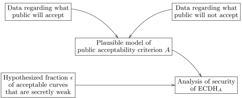
Fig. 1.1. Data flow in this paper. The available data regarding public acceptability is stratified into five different models of the public acceptability criterionA, considered in Sections 3,4,5,6, and7 respectively, with five different shapes of the auxiliary curve data S. The security of eachA is analyzed for variable .

details of secret vulnerabilities, even if we were aware of such vulnerabilities.4 Our goal in this paper is not to evaluate the cost of Eve’s computation, but rather to evaluate the impact of A and upon the cost of Jerry’s computation. For this evaluation it is adequate to use simplified models of secret vulner-abilities. We specify various artificial curve criteria that have no connection to vulnerabilities but that are satisfied by (E, P, S) with probability for various sizes of . We then evaluate how difficult it is for Jerry to find (E, P, S) that satisfy these criteria and that have A(E, P, S) = 1.

The possibilities that we analyze for A are models built from data regarding what the public will accept. See Figure1.1for the data flow. Consider, for exam-ple, the following data: the public has accepted without complaint the constants sin(1),sin(2), . . . ,sin(64) in MD5, the constants √2,√3,√5,√10 in SHA-1, the constants √3

2,√3

3,√3

5,√3

7 in SHA-2, the constant (1 +√5)/2 in RC5, the con-stant e = exp(1) in Brainpool, the constant 1/π in ARIA, etc. All of these constants are listed in [51] as examples of “nothing up my sleeve numbers”. Extrapolating from this data, we confidently predict that the public would ac-cept, e.g., the constant cos(1) used in our example curve BADA55-VPR-224 in Section 5. Enumerating a complete list of acceptable constants would require more systematic psychological experiments, so we have chosen a conservative acceptability function A in Section 5 that allows just 17 constants and their reciprocals.

The reader might object to our specification of ECDHA as implicitly assum-ing that the party sabotagassum-ing curve choices to protect society is the same as the party issuing curve standards to be used by Alice and Bob. In reality, these two

4

(5)

parties are different, and having the first party exercise sufficient control over the second party is often a delicate exercise in finesse. See, for example, [31,20]. 1.2. Organization. Section 2 reviews the curve attacks known to the public and analyzes the probability that a curve resists these attacks; this probability has an obvious impact on the cost of generating curves. Section3, as a warm-up, shows how to manipulate curve choices when A merely checks for these public vulnerabilities.

Section 4 shows how to manipulate “verifiably random” curve choices ob-tained by hashing seeds. Section 5shows how to manipulate “verifiably pseudo-random” curve choices obtained by hashing “nothing-up-my-sleeves numbers”. Section 6 shows how to manipulate “minimal” curve choices. Section 7 shows how to manipulate “the fastest curve”.

1.3. Research contributions of this paper. We appear to be the first to formally introduce the three-party protocol ECDHA. The general idea of Sec-tion4is not new, but our cost analysis is new. We are the first to implement the attack,5 showing how little computer power is necessary to target highly unusual curve properties. Our theoretical and experimental analysis of the percentage of secure curves (see Section 2) is also new.

The general idea of Sections 5 and 6 is new. We are the first to show that curves using so-called “nothing-up-my-sleeves numbers” can very well be ma-nipulated to contain a secret vulnerability. We present concrete ways to gain many bits of freedom and analyze how likely a new vulnerability needs to be in order to hide in this framework. It is surprising that millions of curves can be generated by plausible variations of the Brainpool [14] curve-generation proce-dure, and that hundreds of thousands of curves can be generated by plausible variations of the Microsoft [13] curve-generation procedure.

As discussed in Sections 4.2 and 5, we encourage Jerry to experimentally study the exact boundary of what the public will accept. In followup work to Section5, Aumasson has posted a “Generator of ‘nothing-up-my-sleeve’ (NUMS) constants” that “generates close to 2 million constants, and is easily tweaked to generate many more”. See [4].

2 Pesky public researchers and their security analyses

One obstacle Jerry has to face in deploying his backdoored elliptic curves is that public researchers have raised awareness of certain weaknesses an elliptic curve may have. Once sufficient awareness of a weakness has been raised, many standardization committees will feel compelled to mention that weakness in their standards. This in turn may alert the targeted users, i.e., the general public: some users will check what standards say regarding the properties that an elliptic curve should have or should not have.

The good thing about standards is that there are so many to choose from. Standards evaluating or claiming the security of various elliptic curves include

(6)

ANSI X9.62 (1999) [1], IEEE standard P1363 (2000) [29], Certicom SEC 1 v1 (2000) [16], Certicom SEC 2 v1 (2000) [17], NIST FIPS 186-2 (2000) [41], ANSI X9.63 (2001) [2], Brainpool (2005) [14], NSA Suite B (2005) [43], Certicom SEC 1 v2 (2009) [18], Certicom SEC 2 v2 (2010) [19], OSCCA SM2 (2010) [44,45], ANSSI FRP256V1 (2011) [3], and NIST FIPS 186-4 (2013) [42]. These stan-dards vary in many details, and also demonstrate important variations in public acceptability criteria, an issue explored in depth later in this paper.

Unfortunately for Jerry, some public criteria have become so widely known that all of the above standards agree upon them. Jerry’s curves need to satisfy these criteria. This means not only that Jerry will be unable to use these public attacks as back doors, but also that Jerry will have to bear these criteria in mind when searching for a vulnerable curve. Perhaps the vulnerability known secretly to Jerry does not occur in curves that satisfy the public criteria; on the other hand, perhaps this vulnerability occurs more frequently in curves that satisfy the public criteria than in general curves. The chance of a curve being vulnerable is defined relative to the curves that the public will accept.

This section has three goals:

– Review these standard criteria for “secure” curves, along with attacks those pesky researchers have found. Jerry must be careful, when designing and justifying his curve, to avoid revealing attacks outside this list; such attacks are not known to the public.

– Analyze the probabilityδthat a curve satisfies the standard security criteria. This has a direct influence on Jerry’s curve-generation cost. Two particular criteria, “small cofactor” and “small twist cofactor”, are satisfied by only a small fraction of curves.

– Analyze the probability that a curve is actually feasible to break by various public attacks. It turns out that there are many probabilities on different scales, showing that one should also consider a range of probabilities for Jerry’s secret vulnerability. Recall thatis, by definition, the probability that curves passing the public criteria are secretly vulnerable to Jerry’s attack. Each curve that Jerry tries works with probability onlyδ. The number of curves that Jerry can afford to try and is allowed to try depends on various optimiza-tions and constraints analyzed later in this paper; combining this number withδ immediately reveals Jerry’s overall success chance at creating a vulnerable curve that passes the public criteria, avoiding alarms from the pesky researchers. 2.1. Warning: math begins here. For simplicity we cover only prime fields

here. If Jerry’s secret vulnerability works only in binary fields then we would expect Jerry to have a harder time convincing his targets to use vulnerable curves, although of course he should try.

(7)

Write |E(_Fp)| for the number of points on E defined over Fp, and write |E(_Fp)| asp+ 1−t. Hasse’s theorem (see, e.g., [49]) states that|E(_Fp)| is in the “Hasse interval” [p+ 1−2√p, p+ 1 + 2√p]; i.e.,t is between −2√p and 2√p.

Define ` as the largest prime factor of |E(_Fp)|, and define the “cofactor” h as |E(_Fp)|/`. Let P be a point on E of order `.

2.2. Review of public ECDLP security criteria. Elliptic curve cryptog-raphy is based on the believed hardness of the elliptic-curve discrete-logarithm problem (ECDLP), i.e., the belief that it is computationally infeasible to find a scalar k satisfying Q=kP given a random multiple Q of P on E. The state-of-the-art public algorithm for solving the ECDLP is Pollard’s rho method (with negation), which on average requires approximately 0.886√` point additions. Most publications require the value ` to be large; for example, the SafeCurves web page [9] requires that 0.886√` >2100_.

Some standards put upper limits on the cofactorh, but the limits vary. FIPS 186-2 [41, page 24] claims that “for efficiency reasons, it is desirable to take the cofactor to be as small as possible”; the 2000 version of SEC 1 [16, page 17] required h≤4; but the 2009 version of SEC 1 [18, pages 22 and 78] claims that there are efficiency benefits to “some special curves with cofactor larger than four” and thus requires merelyh ≤2α/8 for security level 2α. We analyze a few possibilities for h and later give examples with h = 1; many standard curves have h = 1.

Another security parameter is the complex-multiplication field discriminant (CM field discriminant) which is defined as D= (t2−4p)/s2 if (t2−4p)/s2 ≡1 (mod 4) or otherwiseD= 4(t2−4p)/s2, wheretis defined asp+ 1− |E(_Fp)|and s2 is the largest square dividingt2−4p. One standard, Brainpool, requires |D| to be large (by requiring a related quantity, the “class number”, to be large). However, other standards do not constrain D, there are various ECC papers choosing curves where D is small, and the only published attacks related to the size of D are some improvements to Pollard’s rho method on a few curves. If Jerry needs a curve with small D then it is likely that Jerry can convince the public to accept the curve. We do not pursue this possibility further.

All standards prohibit efficient additive and multiplicative transfers. An ad-ditive transfer reduces the ECDLP to an easy DLP in the adad-ditive group of _Fp; this transfer is applicable when ` equals p. A degree-k multiplicative transfer reduces the ECDLP to the DLP in the multiplicative group of _Fpk where the

problem can be solved efficiently using index calculus if the embedding degree k is not too large; this transfer is applicable when ` divides pk−1. All standards prohibit ` = p, ` dividing p−1, ` dividing p+ 1, and ` dividing various larger pk−1; the exact limit on k varies from one standard to another.

2.3. ECC security vs. ECDLP security. The most extensive public list of requirements is on the SafeCurves web page [9]. SafeCurves covers hardness of ECDLP, generally imposing more stringent constraints than the standards listed in Section2.2; for example, SafeCurves requires the discriminant D of the CM field to satisfy |D| > 2100 _{and requires the order of} _p _modulo _`_{, i.e., the}

(8)

Jerry is that SafeCurves also covers the general security of ECC, i.e., the security of ECC implementations.

For example, if an implementor of NIST P-224 ECDH uses the side-channel-protected scalar-multiplication algorithm recommended by Brier and Joye [15], reuses an ECDH key for more than a few sessions,6 _{and fails to perform a} mod-erately expensive input validation that has no impact on normal usage,7 then a twist attack finds the user’s secret key using approximately 258 _{elliptic-curve}

additions. See [9] for details. SafeCurves prohibits curves with lowtwist security, such as NIST P-224.

Luckily for Jerry, the other standards listed above focus on ECDLP hard-ness and impose very few additional ECC security constraints. This gives Jerry the freedom (1) to choose a non-SafeCurves-compliant curve that encourages insecure ECC implementations even if ECDLP is difficult, and (2) to deny that there are any security problems. Useful denial text can be found in a May 2014 presentation [40] from NIST: “The NIST curves do NOT belong to any known class of elliptic curves with weak security properties. No sufficiently large classes of weak curves are known.”

Unfortunately, there is some risk that twist-security and other SafeCurves criteria will be added to future standards.8 This paper considers the possibility that Jerry is forced to generate twist-secure curves; it is important for Jerry to be able to sabotage curve standards even under the harshest conditions. Obviously it is also preferable for Jerry to choose a curve for whichall implementations are insecure, rather than merely a curve that encourages insecure implementations. Twist-security requires the twist E0 of the original curve E to be secure. If |E(_Fp)|=p+1−tthen|E0(_Fp)|=p+1+t. Define`0 as the largest prime factor of p+ 1 +t. SafeCurves requires 0.886√`0 _>₂100 _{to prevent Pollard’s rho method;}

`0 6= p to prevent additive transfers; and p having order at least (`0 −1)/100 modulo `0 to prevent multiplicative transfers. SafeCurves also requires various “combined attacks” to be difficult; this is automatic when cofactors are very small, i.e. when (p+ 1−t)/` and (p+ 1 +t)/`0 are very small integers.

2.4. The probability δ of passing public criteria.This subsection analyzes the probability of random curves passing the public criteria described above.

We begin by analyzing how many random curves have small cofactors. As illustrations we consider cofactorsh= 1,h= 2, andh= 4. Note that, for primes 6 _[₂₀_{, Section 4.2] reports that Microsoft’s SChannel automatically reuses “ephemeral”}

keys “for two hours”.

7 _{A very recent paper [}₃₀_{] reports complete breaks of the ECC implementations in}

Bouncy Castle and Java Crypto Extension, precisely because those implementations fail to validate input points.

(9)

plarge enough to pass a laugh test (at least 224 bits), curves with these cofactors automatically satisfy the requirement 0.886√` >2100; in other words, requiring a curve to have a small cofactor supersedes requiring a curve to meet minimal public requirements for security against Pollard’s rho method.

Let π(x) be the number of primes p ≤ x, and let π(S) be the number of primes p in a set S. The prime-number theorem states that the ratio between π(x) and x/logx converges to 1 as x→ ∞, where log is the natural logarithm. Explicit bounds such as [46] are not sufficient to count the number of primes in a short interval I = [x−y, x], but there is nevertheless ample experimental evidence that π(I) is very close to y/logx when y is larger than √x.

The number of integers in I of the form `,2`, or 4`, where ` is prime, is the same as the total number of primes in the intervals I1 = [x−y, x], I2 =

[(x−y)/2, x/2] andI4 = [(x−y)/4, x/4], namely

π(I1) +π(I2) +π(I4)≈

y logx +

y/2 log (x/2) +

y/4 log (x/4) =

X

h∈{1,2,4}

y/h log(x/h).

Take x =p+ 1 + 2√p and y = 4√p to see that the number of such integers in the Hasse interval is approximatelyP

h∈{1,2,4}(4 √

p/h)/(log ((p+ 1 + 2√p)/h)). The total number of integers in the Hasse interval is almost exactly 4√p, so the chance of an integer in the interval having the form`, 2`, or 4` is approximately

X

h∈{1,2,4}

1

hlog ((p+ 1 + 2√p)/h). (1)

This does not imply, however, that the same approximation is valid for the number of points on a random elliptic curve. It is known, for example, that the number of points on an elliptic curve is odd with probability almost exactly 1/3, not 1/2; this suggests that the number is prime less often than a uniformly distributed random integer in the Hasse interval would be.

A further difficulty is that we need to know not merely the probability that the cofactorhis small, but the joint probability that bothhandh0 = (p+1+t)/`0 are small. Even if one disregards the subtleties in the distribution ofp+1−t, one should not expect (e.g.) the probability thatp+ 1−t is prime to be independent of the probability thatp+ 1 +t is prime: for example, if one quantity is odd then the other is also odd.

Galbraith and McKee in [25, Conjecture B] formulated a precise conjecture for the probability of any particularh (called “k” there). Perhaps the techniques of [25] can be extended to formulate a conjecture for the probability of any par-ticular pair (h, h0). However, no such conjectures appear to have been formulated yet, let alone tested.

To collect facts we performed the following experiment: takep= 2224−296₊₁

(the NIST P-224 prime, which is also used in the following sections), and count the number of points on 1000000 curves. Specifically, we took the curves y2 = x3 ₋₃_x _{+ 1 through} _y2 ₌ _x3 ₋₃_x_{+ 1000001, skipping the non-elliptic curve}

(10)

behave nonrandomly, but the same type of nonrandomness appears naturally in Section 6, so this is a relevant experiment. Furthermore, the simple description makes the experiment easy to reproduce.

Within this sample we found probability 0.003705 of h = 1, probability 0.002859 ofh = 2, and probability 0.002372 ofh = 4, with total 0.008936≈2−7_.

We also found, unsurprisingly, practically identical probabilities for the twist cofactor: probability 0.003748 of h0 = 1, probability 0.002902 of h0 = 2, and probability 0.002376 of h0 = 4, with total 0.009026.

For comparison, Formula (1) evaluates to approximately 0.011300 (about 25% too optimistic), built from 0.006441 for h= 1 (about 74% too optimistic), 0.003235 for h = 2 (about 13% too optimistic), and 0.001625 for h = 4 (about 32% too pessimistic).

In our sample we found probability 0.000049 that simultaneouslyh ∈ {1,2,4} and h0 ∈ {1,2,4}. This provides reasonable confidence, although not a guaran-tee, that the events h ∈ {1,2,4} and h0 ∈ {1,2,4} are statistically dependent: independence would mean that the joint event would occur with probability approximately 0.000081, so a sample of size 1000000 would contain ≤49 such curves with probability under 0.0001.

We found probability 0.000032 ≈ 2−15 of h = h0 = 1. Our best estimate, with the caveat of considerable error bars, is therefore that Jerry must try about 215 curves before finding one with h = h0 = 1. If Jerry is free to neglect twist security, searching only for h = 1, then the probability jumps by two orders of magnitude to about 2−8. If Jerry is allowed to take any h ∈ {1,2,4} then the probability is about 2−7.

These probabilities are not noticeably affected by the SafeCurves require-ments regarding the CM discriminant, additive transfers, and multiplicative transfers. Specifically, random curves have a large CM field discriminant, prac-tically always meeting the SafeCurves CM criterion; none of our experiments found a CM field discriminant below 2100. We also found, unsurprisingly, no curves with`=p. As for multiplicative transfers: Luca, Mireles, and Shparlinski gave a theoretical estimate [37] for the probability that for a sufficiently large prime number p and a positive integer K with logK = O(log logp) a randomly chosen elliptic curve E(_Fp) has embedding degree k ≤ K; this result shows that curves with small embedding degree are very rare. The SafeCurves bound K = (`−1)/100 is not within the range of applicability of their theorem, but experimentally we found that about 99% of all curves had a high embedding degree ≥K.

2.5. The probabilities for various feasible attacks.We now consider vari-ous feasible public attacks as models of Jerry’s secret vulnerability. Specifically, for each attack, we evaluate the probability that the attack works against curves that were not chosen to be secure against this type of attack. Any such proba-bility is a reasonable guess for an of interest to Jerry.

At the low end is, e.g., an additive transfer, applying only to curves having exactlyp points. The probability here is roughlyp−1/2_{: e.g., below 2}−100 _{for the}

(11)

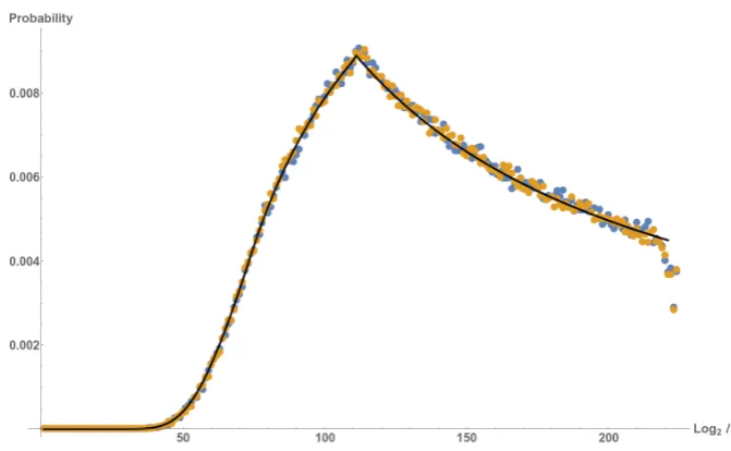
Fig. 2.1. Largest prime factor versus the probability. Blue: The regular curves E. Orange: The twists of the curves E. Black: The Dickman estimate. Orange is more visible than blue because orange is plotted on top of blue.

At the high end, most curves fail the “rho” and “twist” security criteria; see Section 2.4. But this does not mean that the curves are feasible to break, or that the breaking cost is low enough for Jerry to usefully apply to billions of targets. These security criteria are extremely cautious, staying far away from anything potentially breakable by these attacks. For example, `≈ 2150 fails the SafeCurves security criteria but still requires about 275 elliptic-curve operations to break by the rho attack, costing roughly 100 million watt-years of energy with current hardware, a feasible but highly nontrivial cost. A much smaller `≈2120 would require about 260 elliptic-curve operations, and breaking 230 targets by standard multiple-target techniques would again require about 275 elliptic-curve operations. Even smaller values of ` are of interest for twist attacks.

The prime-number theorem can be used to estimate the probabilities of var-ious sizes of ` as in Section 2.4, but it loses applicability as ` drops below √p. To estimate the probability for a wider range of` we use the following result by Dickman (see, e.g., [27]). Define Ψ(x, y) as the number of integers ≤ x whose largest prime factor is at most y; these numbers are called y-smooth integers. Dickman’s result is then as follows:

Ψ(x, y)∼xρ(u) as x → ∞, where x=yu.

Hereρ, the “Dickmanρfunction”, satisfiesρ(u) = 1 for 0≤u≤1 and−uρ0(u) = ρ(u −1) for u ≥ 1, where ρ0 means the right derivative. It is not difficult to compute ρ(u) to high accuracy.

(12)

p k= 30 k= 40 k= 50 k= 60 k= 70 k= 80

P-224 prime 2−15.74 2−8.382 2−4.752 2−2.743 2−1.560 2−0.8601

P-256 prime 2−20.47 2−11.37 2−6.730 2−4.132 2−2.551 2−1.557

P-384 prime 2−42.10 2−25.51 2−16.65 2−11.37 2−7.977 2−5.708

P-521 prime 2−68.64 2−43.34 2−29.57 2−21.16 2−15.63 2−11.81

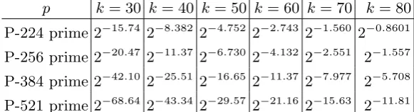
Table 2.2. Estimated probability that an elliptic curve modulo p has largest twist prime at most 22k and second largest twist prime at most 2k, i.e., that an elliptic curve modulopis vulnerable to a twist attack using approximately 2k operations. Estimates rely on the method of [5] to compute asymptotic semismoothness probabilities.

factor has exactly k bits:

Ψ(p+1+2√p,2k)−Ψ(p+1−2√p,2k)−Ψ(p+1+2√p,2k−1)+Ψ(p+1−2√p,2k−1). We divided this by 4√p(the size of the Hasse interval) to obtain the black graph in Figure2.1. We also experimentally computed (for a somewhat smaller sample than in Section2.4) the fraction of curves where` has k bits, and the fraction of curves where`0 hask bits, shown as blue and orange dots in Figure2.1. The dots are below the right end of the graph in Figure 2.1 for the reasons explained in Section2.4; for smaller values of`the estimate closely matches the experimental data.

About 20% of the 224-bit curves have ` < 2100, producing a tolerable rho attack cost, around 250 _{elliptic-curve operations. However,}_ρ₍_u_{) drops rapidly as}

u increases (it is roughly 1/uu), so the chance of achieving this reasonable cost also drops rapidly as the curve size increases. For 256-bit curves the chance is ρ(2.56) ≈0.12 ≈2−3. For 384-bit curves the chance is ρ(3.84) ≈0.0073 ≈2−7. For 512-bit curves the chance is ρ(5.12)≈0.00025≈2−12_.

We now switch from considering rho attacks against arbitrary curves to con-sidering twist attacks against curves with cofactor 1. For a twist attack to fit into 250 elliptic-curve operations, the largest prime`0 dividingp+ 1 +tmust be below 2100, but also the second-largest prime dividingp+ 1 +t must be below 250; see generally [9]. In other words, p+ 1 +t must be (2100,250)-semismooth. Recall that an integer is defined to be (y, z)-semismooth if none of its prime factors is larger than y and at most one of its prime factors is larger than z. The portion of the twist attack corresponding to the second-largest prime is difficult to batch across multiple targets, so it is reasonable to consider even smaller limits for that prime.

(13)

256-bit curves down to 2−29.57 for 521-bit curves. Table 2.2 shows the results of similar computations for several sizes of primes and several limits on feasible attack costs.

To summarize, feasible attacks in the public literature have a broad range of success probabilities against curves not designed to resist those attacks; proba-bilities listed above include 2−4, 2−8, 2−11, 2−16, and 2−25. It is thus reasonable to consider a similarly broad range of possibilities for , the probability that a curve passing public security criteria is vulnerable to Jerry’s secret attack.

3 Manipulating curves

Here we target users with minimal acceptability criteria: i.e., we assume that A(E, P, S) checks only the public security criteria for (E, P) described in Sec-tion2. The auxiliary dataS might be used to communicate, e.g., a precomputed |E(_Fp)| to be verified by the user, but is not used to constrain the choice of (E, P). Curves that pass the acceptability criteria are safe against known at-tacks, but have no protection against Jerry’s secret vulnerability.

3.1. Curves without public justification.Here are two examples of standard curves distributed without any justification for how they were chosen. These examples suggest that there are many ECC users who do in fact have minimal acceptability criteria.

As a first example, we look at the FRP256V1 standard [3] published in 2011 by the Agence nationale de la sécurité des systèmes d’information (ANSSI). This curve is y2 =x3−3x+bover _Fp, where

b=0xEE353FCA5428A9300D4ABA754A44C00FDFEC0C9AE4B1A1803075ED967B7BB73F, p=0xF1FD178C0B3AD58F10126DE8CE42435B3961ADBCABC8CA6DE8FCF353D86E9C03.

Another example is a curve published by the Office of State Commercial Cryptography Administration (OSCCA) in China along with the SM2 algo-rithms in 2010 (cf. [45,44]). The curve is of the same form as the ANSSI one with

b=0x28E9FA9E9D9F5E344D5A9E4BCF6509A7F39789F515AB8F92DDBCBD414D940E93, p=0xFFFFFFFEFFFFFFFFFFFFFFFFFFFFFFFFFFFFFFFF00000000FFFFFFFFFFFFFFFF. Each curveE is also accompanied by a pointP. The curves meet the ECDLP requirements9 reviewed in Section 2. The only further data provided with these curves is data that could also have been computed efficiently by users from the above information. Nothing in the curve documentation suggests any verification that would have further limited the choice of curves.

3.2. The attack.The attack is straightforward. Since the only things that users check are the public security criteria, Jerry can continue generating curves for

9

(14)

a fixed p (either randomly or not) that satisfy the public criteria until he gets one that is vulnerable to his secret attack. Alternatively, Jerry can generate curves vulnerable to his secret attack and check them against the public security criteria. Every attack (publicly) known so far allows efficient computation of vulnerable curves, so it seems likely that the same will be true for Jerry’s secret vulnerability. After finding a vulnerable curve, Jerry simply publishes it.

Of course, Jerry’s vulnerability must not depend on any properties excluded by the public security criteria, and there must be enough vulnerable curves. Enumerating 27 vulnerable curves over _Fp is likely to be sufficient if Jerry can ignore twist-security, and enumerating 215 vulnerable curves over _Fp is likely to be sufficient even if twist-security is required. See Section 2.

Even if Jerry’s curves are less frequent, Jerry can increase his chances by also varying the prime p. To simplify our analysis we do not take advantage of this flexibility in this section: we assume that Jerry is forced to reuse a particu-lar standard prime such as a NIST prime or the ANSSI prime. We emphasize, however, that the standard security requirements do not seriously scrutinize the choice of prime, and existing standards vary in their choices of primes. Any al-lowed variability inpwould also improve the attack in Section5, and we do vary p in Section 6.

3.3. Implementation. We implemented the attack to demonstrate that it is really feasible in practice. In our implementation the same setting as above is adopted and even made more restrictive: the resulting curve should be of the form y2 =x3−3x+b over _Fp, where pis the same as for the ANSSI curve. The public security criteria we consider are all the standard ECDLP security criteria plus twist security, and we further require that both cofactors are 1.

Of course, as explained in the introduction, we will not include any actual secret vulnerability in this white paper. We instead use a highly structured parameter b as an artificial model of a secret vulnerability. We show that we can construct a curve with such ab that passes all the public criteria. In reality, Jerry would select a curve with a secret vulnerability rather than a curve with our artificial model of a vulnerability, and would use a trustworthy curve name such as TrustedCurve-R-256.

Our attack is implemented using the Sage computer algebra system [50]. We took 0x5AFEBADA55ECC5AFEBADA55ECC5AFEBADA55ECC5AFEBADA55ECC5AFEBADA55EC as the start value for b and incremented b until we found a curve that meets the public security criteria. This corresponds to Jerry iteratively checking whether curves that are vulnerable to the secret attack fulfill the public criteria.

As a result we found a desired curve, which we call BADA55-R-256, with b = 0x5AFEBADA55ECC5AFEBADA55ECC5AFEBADA55ECC5AFEBADA55ECC5AFEBADA5A57 af-ter 1131 increments within 78 minutes on a single core of an AMD CPU.10 One 10 _{Note that a} _lucky _{attacker starting from}

0xBADA55BADA55BADA55BADA55BADA55BADA55BADA55BADA55BADA55BADA55BADA is able to find the following secure parameter already within 43 minutes after only 622 increments:

(15)

p = 0xF1FD178C0B3AD58F10126DE8CE42435B3961ADBCABC8CA6DE8FCF353D86E9C03 # standard ANSSI prime k = GF(p)

def secure(A,B):

n = EllipticCurve([k(A),k(B)]).cardinality() return (n.is_prime() and (2*p+2-n).is_prime()

and Integers(n)(p).multiplicative_order() * 100 >= n-1

and Integers(2*p+2-n)(p).multiplicative_order() * 100 >= 2*p+2-n-1)

A = p-3 # standard -3 modulo p

B = 0xBADA55BADA55BADA55BADA55BADA55BADA55BADA55BADA55BADA55BADA55BD48 if secure(A,B):

print ’p’,hex(p).upper() print ’A’,hex(A).upper() print ’B’,hex(B).upper()

# output:

# p F1FD178C0B3AD58F10126DE8CE42435B3961ADBCABC8CA6DE8FCF353D86E9C03 # A F1FD178C0B3AD58F10126DE8CE42435B3961ADBCABC8CA6DE8FCF353D86E9C00

# B BADA55BADA55BADA55BADA55BADA55BADA55BADA55BADA55BADA55BADA55BD48

Fig. 3.1. A procedure to generate the new BADA55-R-256 curve.

can easily check using a computer-algebra system that the curve does meet all the public criteria. It is thus clear that users who only verify public security criteria can be very easily attacked, and Jerry has an easy time if he is working for or is trusted by ANSSI, OSCCA, or a similar organization.

4 Manipulating seeds

Section3deals with the easiest case for Jerry that the users are satisfied verifying public security criteria. However some audiences might demand justifications for the curve choices. In this section, we consider users who are suspicious that the curve parameters might be maliciously chosen to enable a secret attack. Empirically many users are satisfied if they get a hash verification routine as justification; see, e.g., ANSI X9.62 [1], IEEE P1363 [29], SEC 2 [19], or NIST FIPS 186-2 [41]. Hash verification routines mean that Jerry cannot use a very small set of vulnerable curves, but we will show below that he has good chances to get vulnerable curves deployed if they are just somewhat more common. 4.1. Hash verification routine.As the name implies, a hash verification rou-tine involves a cryptographic hash function. The inputs to the rourou-tine are the curve parameters and a seed that is published along with the curve. Usually the seed is hashed to compute a curve parameter or point coordinate. The ways of computing the parameters differ but the public justification is that these bind the curve parameters to the hash value, making them hard to manipulate since the hash function is preimage resistant11. In addition the user verifies a set of public security criteria. We focus on the obstacle that Jerry faces and call curves that can be verified with such routines verifiably hashed curves.

11

(16)

For Jerry’s marketing we do not recommend the phrase “verifiably hashed”: it is better to claim that the curves are totally random (even though this is not what is being verified) and that these curves could not possibly be manipulated (even though Jerry is in fact quite free to manipulate them). For example, ANSI X9.62 [1, page 31] speaks of “selecting an elliptic curve verifiably at random”; SEC 2 [19, copy and paste: page 8 and page 18] claims that “verifiably random parameters offer some additional conservative features” and “that the parame-ters cannot be predetermined”. NIST’s marketing in [41] is not as good: NIST uses the term “pseudo-random curves”.

Below we recall the curve verification routine for the NIST P-curves. The routine is specified in NIST FIPS 186-2 [41].

Each NIST P-curve is of the form y2 = x3 −3x+b over a prime field _Fp and is published with a seed s. The hash function SHA-1 is denoted as SHA1; recall that SHA-1 produces a 160-bit hash value. The bit length of p is denoted by m. We use bin(i) to denote the 20-byte big-endian representation of some integer iand use int(j) to denote the integer with binary expansionj. For given parameters b, p, and s, the verification routine is:

1. Let z ← int(s). Compute hi ← SHA1(si) for 0 ≤ i ≤ v, where si ← bin((z+i) mod 2160) andv =b(m−1)/160c.

2. Let h be the rightmost m−1 bits of h0||h1|| · · · ||hv. Let c←int(h). 3. Verify that b2c=−27 in _Fp.

To generate a verifiably hashed curve one starts with a seed and then follows the same steps 1 and 2 as above. Instead of step 3 one tries to solve for b given c; this succeeds for about 50% of all choices fors. The public perception is that this process is repeated with fresh seeds until the first resulting curve satisfies all public security criteria.

4.2. Acceptability criteria.One might think that the public acceptability cri-teria are defined by the NIST verification routine stated above: i.e.,A(E, P, s) = 1 if and only if (E, P) passes the public security criteria from Section 2 and (E, s) passes the verification routine stated above with seed s and E defined as y2 =x3−3x+b.

However, the public acceptability criteria are not actually so strict. P1363 allows y2 = x3+ax+b without the requirement a = −3. P1363 does require b2c = a3 where c is a hash as above, but neither P1363 nor NIST gives a justification for the relation b2c=a3, and it is clear that the public will accept different relations. For example, the Brainpool curves (see Section 5) use the simpler relations a = g and b= h where g and h are separate hashes. One can equivalently view the Brainpool curves as following the P1363 procedure but using a different hash for c, namely computing c as g3_/h2 _{where again} _g _and _h

(17)

as in Section3. The exact boundaries of public acceptability are complicated and not immediately obvious. We have determined approximations to these bound-aries by extrapolating from existing data (see, e.g., Section5), and we encourage Jerry to carry out large-scale scientific surveys, while taking care to prevent leaks to the public.

4.3. The attack.Jerry begins the attack by defining a public hash verification routine. As explained above, Jerry has some flexibility to modify this routine. This flexibility is not necessary for the rest of the attack in this section (for ex-ample, Jerry can use exactly the NIST verification routine) but a more favorable routine does improve theefficiency of the attack. Our cost analysis below makes a particularly efficient choice of routine.

Jerry then tries one seed after another until finding a seed for which the verifiably hashed curve (1) passes the public security criteria but (2) is subject to his secret vulnerability. Jerry publishes this seed and the resulting curve, pretending that the seed was the first random seed that passed the public security criteria.

4.4. Optimizing the attack.Assume that the curves vulnerable to Jerry’s se-cret attack are randomly distributed over the curves satisfying the public security criteria. Then the success probability that a seed leads to a suitable curve is the probability that a curve is vulnerable to the secret attack times the probability that a curve satisfies the public security criteria. Depending on which condition is easier to check Jerry runs many hash computations to compute candidate b’s, checks them for the easier criterion and only checks the surviving choices for the other criterion. The hash computations and security checks for each seed are independent from other seeds; thus, this procedure can be parallelized with an arbitrary number of parallel computing instances.

We generated a family of curves to show the power of this method and highlight the computing power of hardware accelerators (such as GPUs or Xeon Phis). We began by defining our own curve verification routine and implementing the corresponding secret generation routine. The hash function we use is Keccak with 256-bit output instead of SHA-1. The hash value is c = int(Keccak(s)), and the relation is simply b = c in _Fp. All choices are easily justified: Keccak is the winner of the SHA-3 competition and much more secure than SHA-1; using a hash function with a long output removes the weird order of hashed components that smells suspicious and similarly b=cis as simple and unsuspi-cious as it can get. In reality, however, these choices greatly benefit the attack: the GPUs efficiently search through many seeds in parallel, one single compu-tation of Keccak has a much easier data flow than in the method above, and having b computed without any expensive number-theoretic computation (such as square roots) means that the curve can be tested already on the GPUs and only the fraction that satisfies the first test is passed on to the next stage. Of course, for a real vulnerability we would have to add the cost of checking for that vulnerability, but minimizing overhead is still useful.

(18)

import binascii import simplesha3

hash = simplesha3.keccakc512 # SHA-3 winner with 256-bit output

p = 2^224 - 2^96 + 1 # standard NIST P-224 prime k = GF(p)

def secure(A,B):

def str2int(seed):

return Integer(seed.encode(’hex’),16)

A = p-3

S = ’3CC520E9434349DF680A8F4BCADDA648D693B2907B216EE55CB4853DB68F9165’ B = str2int(hash(binascii.unhexlify(S))) # verifiably random

if secure(A,B):

# output:

# p FFFFFFFFFFFFFFFFFFFFFFFFFFFFFFFF000000000000000000000001 # A FFFFFFFFFFFFFFFFFFFFFFFFFFFFFFFEFFFFFFFFFFFFFFFFFFFFFFFE

# B BADA55ECFD9CA54C0738B8A6FB8CF4CCF84E916D83D6DA1B78B622351E11AB4E

Fig. 4.1.A procedure to generate the new “verifiably random” BADA55-VR-224 curve. Since the hash output is more than 256 bits, we implicitly reduce it modulop.

3x+ b over _Fp, and we consider 3 choices of p: the NIST P-224, P-256, and P-384 primes. (For P-384 we switched to Keccak with 384-bit output.) As a placeholder “vulnerability” we defineE to be vulnerable ifbstarts with the hex-string BADA55EC. This fixes 8 hex digits, i.e., it simulates a 1-out-of-232 _attack.

In addition we require that the curves meet the standard ECDLP criteria plus twist security and have both cofactors equal to 1.

4.5. Implementation. Our implementation uses NVIDIA’s CUDA framework for parallel programming on GPUs. A high-end GPU today allows several thou-sand threads to run in parallel, though at a frequency slightly lower than high-end CPUs. We let each thread start with its own random seed. The threads then hash the seeds in parallel. After hashing, each thread outputs the hash value if it starts with the hex-string BADA55EC. To restart, each seed is simply increased by 1, so no new source of randomness is required. Checking whether outputs from GPUs also satisfy the public security criteria is done by running a Sage [50] script on CPUs. Since only 1 out of 232 curves has the desired pattern, the CPU computation is totally hidden by GPU computation. Longer strings, cor-responding to less likely vulnerabilities, make GPUs even more powerful for our attack scheme.

(19)

p = 2^256 - 2^224 + 2^192 + 2^96 - 1 # standard NIST P-256 prime k = GF(p)

def secure(A,B):

def str2int(seed):

A = p-3

S = ’3ADCC48E36F1D1926701417F101A75F000118A739D4686E77278325A825AA3C6’ B = str2int(hash(binascii.unhexlify(S))) # verifiably random

if secure(A,B):

# output:

# p FFFFFFFF00000001000000000000000000000000FFFFFFFFFFFFFFFFFFFFFFFF # A FFFFFFFF00000001000000000000000000000000FFFFFFFFFFFFFFFFFFFFFFFC

# B BADA55ECD8BBEAD3ADD6C534F92197DEB47FCEB9BE7E0E702A8D1DD56B5D0B0C

Fig. 4.2.A procedure to generate the new “verifiably random” BADA55-VR-256 curve.

Jerry would use a secret vulnerability rather than our artificial “vulnerability”, and would use the name TrustedCurve-VR rather than BADA55-VR.

(20)

p = 2^384 - 2^128 - 2^96 + 2^32 - 1 # standard NIST P-384 prime k = GF(p)

def secure(A,B):

def str2int(seed):

A = p-3

S = ’CA9EBD338A9EE0E6862FD329062ABC06A793575A1C744F0EC24503A525F5D06E’ B = str2int(hash(binascii.unhexlify(S))) # verifiably random

if secure(A,B):

# output:

# p FFFFFFFFFFFFFFFFFFFFFFFFFFFFFFFFFFFFFFFFFFFFFFFFFFFFFFFFFFFFFFFEFFFFFFFF0000000000000000FFFFFFFF # A FFFFFFFFFFFFFFFFFFFFFFFFFFFFFFFFFFFFFFFFFFFFFFFFFFFFFFFFFFFFFFFEFFFFFFFF0000000000000000FFFFFFFC

# B BADA55EC3BE2AD1F9EEEA5881ECF95BBF3AC392526F01D4CD13E684C63A17CC4D5F271642AD83899113817A61006413D

Fig. 4.3.A procedure to generate the new “verifiably random” BADA55-VR-384 curve.

5 Manipulating nothing-up-my-sleeve numbers

There are some particularly pesky researchers who do not shut up even when provided with a verification routine as in the previous section. These researchers might even think of the powerful attack presented in the previous section.

(21)

We have written a Sage implementation, emphasizing simplicity and clarity, of the prime-generation and curve-generation procedures specified in the Brain-pool standard [14, Section 5]. For example, Figure 5.1 (designed to be shown to the public) uses Brainpool’s procedure to generate a 224-bit curve. The output consists of the following “verifiably pseudorandom” integers p, a, b defining an elliptic curve y2 =x3+ax+bover _Fp:

p=0xD7C134AA264366862A18302575D1D787B09F075797DA89F57EC8C0FF

a=0x2B98B906DC245F2916C03A2F953EA9AE565C3253E8AEC4BFE84C659E

b=0x68AEC4BFE84C659EBB8B81DC39355A2EBFA3870D98976FA2F17D2D8D

We have added underlines to point out an embarrassing collision of substrings, obviously quite different from what one expects in “pseudorandom” strings.

What happened here is that the Brainpool procedure generates each ofaand b as truncations of concatenations of various hash outputs (since the selected hash function, SHA-1, produces only 160-bit outputs), and there was a collision in the hash inputs. Specifically, Brainpool uses the same seed-increment function for three purposes: searching for a suitable a; moving from a to b; and moving within the concatenations. The first hash used in the concatenation fora was fed through this increment function to obtain the second hash, and was fed through the same increment function to obtain the first hash used in the concatenation for b, producing the overlap visible above.

A reader who checks the Brainpool standard [14] will find that the 224-bit curve listed there does not have the same (a, b), and does not have this overlap. The reason for this is that, astonishingly, the 224-bit standard Brainpool curve was not actually produced by the standard Brainpool procedure. In fact, although the reader will find overlaps in the standard 192-bit, 256-bit, 384-bit, and 512-bit Brainpool curves, none of the standard Brainpool curves below 512 bits were produced by the standard Brainpool procedure. In the case of the 160-bit, 224-bit, 320-bit, and 384-bit Brainpool curves, one can immediately demonstrate this discrepancy by observing that the gap listed between “seedA” and “seed B” in [14, Section 11] is larger than 1, while the standard procedure always produces a gap of exactly 1.

A procedure that actually does generate the Brainpool curves appeared a few years later in the Brainpool RFC [34] and is reimplemented in Figure 5.2. For readers who do not enjoy playing a “spot the differences” game between Figures 5.1and 5.2, we explain how the procedures differ:

– The procedure in [34] assigns seeds to an (a∗ab∗b)∗ pattern. It tries consec-utive seeds for a until finding that −3/a is a 4th power, then tries further seeds for b until finding that b is not a square, then checks whether the re-sulting curve meets Brainpool’s security criteria. If this fails, it goes back to trying further seeds for a etc.

(22)

import hashlib # for a PRNG, SHA-1 is standard and sufficiently secure def hash(seed): h = hashlib.sha1(); h.update(seed); return h.digest() seedbytes = 20 # 160-bit size for seed, determined by SHA-1 output size

# 224-bit prime p produced by very similar procedure, shown in separate file p = 0xD7C134AA264366862A18302575D1D787B09F075797DA89F57EC8C0FF

k = GF(p); R.<x> = k[]

def secure(A,B):

if k(B).is_square(): return False

n = EllipticCurve([k(A),k(B)]).cardinality() return (n < p and n.is_prime()

and Integers(n)(p).multiplicative_order() * 100 >= n-1)

def int2str(seed,bytes): # standard big-endian encoding of integer seed return ’’.join([chr((seed//256^i)%256) for i in reversed(range(bytes))])

def str2int(seed):

def update(seed): # add 1 to seed, viewed as integer return int2str(str2int(seed) + 1,len(seed))

def fullhash(seed):

return str2int(hash(seed) + hash(update(seed))) % 2^223

def real2str(seed,bytes): # most significant bits of real number between 0 and 1 return int2str(Integer(floor(RealField(8*bytes+8)(seed)*256^bytes)),bytes)

nums = real2str(exp(1)/16,7*seedbytes) # enough bits for all curve sizes S = nums[2*seedbytes:3*seedbytes] # previous bytes are used for 160 and 192 while True:

A = fullhash(S)

if not (k(A)*x^4+3).roots(): S = update(S); continue S = update(S)

B = fullhash(S)

if not secure(A,B): S = update(S); continue print ’p’,hex(p).upper()

print ’A’,hex(A).upper() print ’B’,hex(B).upper() break

# output:

# p D7C134AA264366862A18302575D1D787B09F075797DA89F57EC8C0FF # A 2B98B906DC245F2916C03A2F953EA9AE565C3253E8AEC4BFE84C659E # B 68AEC4BFE84C659EBB8B81DC39355A2EBFA3870D98976FA2F17D2D8D

Fig. 5.1. An implementation of the Brainpool standard procedure [14, Section 5] to generate a 224-bit curve.

meets Brainpool’s security criteria. If this fails, it goes back to trying further seeds for a etc.

(23)

# 224-bit prime p produced by very similar procedure, shown in separate file p = 0xD7C134AA264366862A18302575D1D787B09F075797DA89F57EC8C0FF

k = GF(p); R.<x> = k[]

def secure(A,B):

n = EllipticCurve([k(A),k(B)]).cardinality() return (n < p and n.is_prime()

def str2int(seed):

def fullhash(seed):

return str2int(hash(seed) + hash(update(seed))) % 2^223

nums = real2str(exp(1)/16,7*seedbytes) # enough bits for all curve sizes S = nums[2*seedbytes:3*seedbytes] # previous bytes are used for 160 and 192 while True:

A = fullhash(S)

if not (k(A)*x^4+3).roots(): S = update(S); continue while True:

S = update(S) B = fullhash(S)

if not k(B).is_square(): break

print ’A’,hex(A).upper() print ’B’,hex(B).upper() break

# output:

# p D7C134AA264366862A18302575D1D787B09F075797DA89F57EC8C0FF # A 68A5E62CA9CE6C1C299803A6C1530B514E182AD8B0042A59CAD29F43 # B 2580F63CCFE44138870713B1A92369E33E2135D266DBB372386C400B

Fig. 5.2.An implementation of a procedure that, unlike Figure5.1, actually generates thebrainpool224r1 curve.

negligible probability of failing, such as having large CM field discriminant (see Section 2); these criteria are trivially verified after the fact.

(24)

inter-import sys

def str2int(seed):

sizes = [160,192,224,256,320,384,512] S = real2str(pi/16,len(sizes)*seedbytes)

primeseeds = [S[i:i+seedbytes] for i in range(0,len(S),seedbytes)] S = real2str(exp(1)/16,len(sizes)*seedbytes)

curveseeds = [S[i:i+seedbytes] for i in range(0,len(S),seedbytes)]

for j in range(len(sizes)): L,S = sizes[j],primeseeds[j] v = (L-1)//160

def fullhash(seed,bits): h = hash(seed)

for i in range(v): seed = update(seed); h += hash(seed) return str2int(h) % 2^bits

Fig. 5.3.Part 1 of 2: A complete procedure to generate the Brainpool standard curves. Continued in Figure 5.4.

esting possibility for Jerry. We do not explore this line of thought further: we make the worst-case assumption that future curves will be verified by the public, using tools that Jerry is unable to corrupt.

The Brainpool standard also includes the following statement [14, page 2]: “It is envisioned to provide additional curves on a regular basis for users who wish to change curve parameters regularly, cf. Annex H2 of [X9.62], paragraph ‘Elliptic curve domain parameter cryptoperiod considerations’.” However, the procedure for generating further “verifiably pseudorandom” curves is not discussed. One possibility is to continue the original procedure past the first (a, b) pair, but this makes new curves more and more expensive to verify. Another possibility is to replace e by a different natural constant.

5.2. The BADA55-VPR-224 procedure. We now present a new and im-proved verifiably pseudorandom 224-bit curve, VPR-224. BADA55-VPR-224 uses the standard NIST P-224 prime, i.e., p= 2224−296+ 1.

(25)

while True:

p = fullhash(S,L)

while not (p % 4 == 3 and p.is_prime()): p += 1 if 2^(L-1) - 1 < p and p < 2^L: break

S = update(S)

k = GF(p) R.<x> = k[]

def secure(A,B):

E = EllipticCurve([k(A),k(B)]) for q in [2,3,5,7]:

# quick check whether q divides n, without computing n for r,e in E.division_polynomial(q).roots():

if E.is_x_coord(r): return False n = E.cardinality()

return (n < p and n.is_prime()

S = curveseeds[j] while True:

A = fullhash(S,L-1)

if not (k(A)*x^4+3).roots(): S = update(S); continue while True:

S = update(S) B = fullhash(S,L-1)

if not k(B).is_square(): break

print ’A’,hex(A).upper() print ’B’,hex(B).upper() sys.stdout.flush() break

Fig. 5.4.Part 2 of 2: A complete procedure to generate the Brainpool standard curves. Continued from Figure 5.3.

Brainpool already generates seeds using exp(1) = e and generates primes using arctan(1) = π/4, and MD5 already uses sin(1), so we use cos(1). We eliminate Brainpool’s contrived, complicated12 search pattern for a: we simply count upwards, trying every seed for a, until finding the first secure (a, b). The full 160-bit seed for a is the 32-bit counter followed by cos(1). We complement this seed to obtain the seed for b, ensuring maximal difference between the two seeds.

Figure 5.5 is a Sage script implementing the BADA55-VPR-224 generation procedure. This procedure is simpler and more natural than the Brainpool pro-cedure in Figure 5.2. Here is the resulting curve:

(26)

import simplesha3

hash = simplesha3.sha3512 # SHA-3 standard at maximum security level

seedbytes = 20 # standard 160-bit size for seed

def secure(A,B):

def str2int(seed):

def complement(seed): # change all bits, eliminating Brainpool-type collisions return ’’.join([chr(255-ord(s)) for s in seed])

def real2str(seed,bytes): # most significant bits of real number between 0 and 1 return int2str(Integer(RealField(8*bytes)(seed)*256^bytes),bytes)

sizeofint = 4 # number of bytes in a 32-bit integer nums = real2str(cos(1),seedbytes - sizeofint)

for counter in xrange(0,256^sizeofint): S = int2str(counter,sizeofint) + nums T = complement(S)

A = str2int(hash(S)) B = str2int(hash(T)) if secure(A,B):

print ’p’,hex(p).upper() print ’A’,hex(A).upper() print ’B’,hex(B).upper() break

# output:

# p FFFFFFFFFFFFFFFFFFFFFFFFFFFFFFFF000000000000000000000001

# A 7144BA12CE8A0C3BEFA053EDBADA555A42391FC64F052376E041C7D4AF23195EBD8D83625321D452E8A0C3BB0 # A048A26115704E45DCEB346A9F4BD9741D14D49

# B 5C32EC7FC48CE1802D9B70DBC3FA574EAF015FCE4E99B43EBE3468D6EFB2276BA3669AFF6FFC0F4C6AE4AE2E5 # D74C3C0AF97DCE17147688DDA89E734B56944A2

Fig. 5.5.A procedure to generate the new “verifiably pseudorandom” BADA55-VPR-224 curve. Compare Figure 5.2.

an easy explanation: two hashes in the Brainpool procedure were visibly given the same input. The surprising appearance of the 24-bit stringBADA55inaabove has no such easy explanation. There are 128 hexadecimal digits ina, so one expects this substring to appear anywhere within a with probability 123/224 ≈2−17.

(27)

for deriving the seed: i.e., each procedure is defined by a combination of hash function, seed length, etc. The exact number of choices available in any partic-ular dimension is relatively unimportant; what is important is the exponential effect from combining many dimensions.

Since 220 is far above 217, it is unsurprising that our “vulnerability” appeared in quite a few of these procedures. We selected one of those procedures and presented it as Section 5.2as an example of what could be shown to the public. See Figure5.6for another example13of such a procedure, generating a BADA55-VPR2-224 curve, starting from e instead of cos(1). We could have easily chosen a more restrictive “vulnerability”.

The structure of this attack means that Jerry can use the same attack to target a real vulnerability that has probability 2−17, or (with reasonable success chance) even 2−20_{, perhaps even reusing our database of curves. As in}

Sec-tion3and Section 4, Jerry should use the name TrustedCurve-VPR rather than BADA55-VPR.

In this section we do not manipulate the choice of prime, the choice of curve shape, the choice of cofactor criterion, etc. Taking advantage of this flexibility (see Section 6) would increase the number of natural-sounding Brainpool-like procedures above 230_.

Our experience is that Alice and Bob, when faced with a single procedure such as Section 5.2 (or Section 5.1), find it extremely difficult to envision the entire space of possible procedures (they typically see just a few dimensions of flexibility), and find it inconceivable that the space could have size as large as 220, never mind 230. This is obviously a helpful phenomenon for Jerry.

5.4. Manipulating bit-extraction procedures.Consider the problem of ex-tracting a fixed-length string of bits from (e.g.) the constant e = exp(1) = 2.71828. . .= (10.10110111. . .)2. Here are several plausible options for the

start-ing bit position:

– Start with the most significant bit: i.e., take bits of e at bit positions 21, 20, 2−1, 2−2, etc.

– Start immediately after the binary point: i.e., take bits of e at bit positions 2−1, 2−2, etc. For some constants this is identical to the first option: consider, e.g., the first MD5 constant sin(1) = 0.84. . ..

– Start with the most significant nibble: i.e., take bits ofe at bit positions 23, 22, 21, 20, 2−1, 2−2, etc.

– Start with the most significant byte: i.e., take bits of e at bit positions 27, 26, 25, etc.

(28)

import simplesha3 # Keccak, the SHA-3 winner

hash = simplesha3.keccakc1024 # maximum security level: 512-bit output seedbytes = 64 # maximum-security 512-bit seed, same size as output

def secure(A,B):

def int2str(seed,bytes): # standard little-endian encoding of integer seed return ’’.join([chr((seed//256^i)%256) for i in range(bytes)])

def str2int(seed):

return sum([ord(seed[i])*256^i for i in range(len(seed))])

def rotate(seed): # rotate seed by 1 bit, eliminating Brainpool-like collisions x = str2int(seed)

x = 2*x + (x >> (8*len(seed)-1)) return int2str(x,len(seed))

counterbytes = 3 # minimum number of bytes needed to guarantee success nums = real2str(exp(1)/4,seedbytes - counterbytes)

for counter in xrange(0,256^counterbytes): S = int2str(counter,counterbytes) + nums R = rotate(S)

A = str2int(hash(R)) B = str2int(hash(S)) if secure(A,B):

print ’p’,hex(p).upper() print ’A’,hex(A).upper() print ’B’,hex(B).upper() break

# output:

# p FFFFFFFFFFFFFFFFFFFFFFFFFFFFFFFF000000000000000000000001

# A 8F0FF20E1E3CF4905D492E04110683948BFC236790BBB59E6E6B33F24F348ED2E16C64EE79F9FD27E9A367FF6 # 415B41189E4FB6BADA555455DC44C4F87011EEF

# B E85067A95547E30661C854A43ED80F36289043FFC73DA78A97E37FB96A2717009088656B948865A660FF3959 # 330D8A1CA1E4DE31B7B7D496A4CDE555E57D05C

Fig. 5.6.A procedure to generate the new “verifiably pseudorandom” BADA55-VPR2-224 curve. Compare Figure 5.5.

– Start with the byte at position 0. In the case of e this is the same as the fourth option. In the case of sin(1) this means prepending 8 zero bits to the fourth option.

These options can be viewed as using different maps from real numbers x to real numbers y with 0 ≤ y < 1: the first map takes x to |x|/2blog2|x|c, the

(29)

We implemented the first, second, and fourth options; for an average constant this produced slightly more than 2 distinct possibilities for real numbers y.

Jerry can easily get away with extracting ak-bit integer fromyby truncation (i.e.,2ky) or by rounding (i.e.,2ky). Jerry can defend truncation (which has fundamentally lower accuracy) as simpler, and can defend rounding as being quite standard in mathematics and the physical sciences; but we see no reason to believe that Jerry would be challenged in the first place. We implemented both options, gaining a further factor of 1.5.

Actually, Brainpool uses the bit position indicated above only for the low-security 160-bit Brainpool curve (which Jerry can disregard as already being a non-problem for Eve). As shown in Figure 5.3, Brainpool shifts to subsequent bits of e for the 192-bit curve, then to further bits for the 224-bit curve, etc. Brainpool uses 160 bits for each curve (see below), so the seed for the 256-bit curve (which Jerry can reasonably guess would be the most commonly used curve) is shifted by 480 bits. This number 480 depends on how many lower security levels are allocated (an obvious target of manipulation), and on exactly how many bits are allocated to those seeds. A further option, pointed out in [39] by Merkle (Brainpool RFC co-author), is to reverse the order of curve sizes; the number 480 then depends on how many higher security levels are allocated. Yet another option is to put curve sizes in claimed order of usage. We did not implement any of the options described in this paragraph.

5.5. Manipulating choices of hash functions.The latest (July 2013) revision of the NIST ECDSA standard [42, Section 6.1.1] specifically requires that “the security strength of a hash function used [for curve generation] shall meet or exceed the security strength associated with the bit length”. The original NIST curves are exempted from this rule by [42, footnote 2], but this rule prohibits SHA-1 for (e.g.) new 224-bit curves. On the other hand, a more recent Brainpool-related curve-selection document [39] states that “For a PRNG, SHA-1 was (and still is) sufficiently secure.”

Jerry has at least 10 plausible options for standard hash functions used to generate (e.g.) 256-bit curves:

– SHA-1. “We follow the Brainpool standard. What matters is preimage resis-tance, and SHA-1 still provides more than 2128 preimage resistance.” – SHA-256. “The trusted, widely deployed SHA-256 standard.”

– SHA-384. “SHA-2 at the security level required to handle both sizes of Suite B curves.”

– SHA-512. “The maximum-security SHA-512 standard.” – SHA-512/256. “NIST’s standard wide-pipe hash function.”

– SHA3-256. “The state-of-the-art SHA-3 standard at a 2128 security level.” – SHA3-384. “The state-of-the-art SHA-3 standard, at the security level

re-quired to handle both sizes of Suite B curves.”

– SHA3-512. “The maximum-security state-of-the-art SHA3-512 standard.” – SHAKE128. “The state-of-the-art SHA-3 standard at a 2128 _{security level,}