© The Authors, published by EDP Sciences. This is an open access article distributed under the terms of the Creative Commons
Attribution License 4.0 (http://creativecommons.org/licenses/by/4.0/).
Local reconstruction algorithms in the cathode strip
cham-bers of CMS
Mirena
Paneva
1
,
∗
on behalf of the CMS Collaboration
1
University of California, Riverside (USA)
Abstract.
The design of the CMS detector is optimized for muon
measure-ments. The muon system consists of gas ionization detector technologies.
Cath-ode Strip Chambers (CSC) with both tracking and triggering capabilities are
in-stalled in the forward region. The first stage of muon reconstruction uses
infor-mation from individual muon chambers and is thus called local reconstruction,
in contrast to a subsequent global reconstruction where the information from
all detectors is combined. First, 2-dimensional spatial points (rechits)
describ-ing where a muon crosses the CSC layers are built from the electrical signals
induced by the charged particle traversing the chamber. Next, from the
recon-structed hits, straight-line track segments are built within each chamber. Local
reconstruction becomes particularly challenging at high instantaneous
luminosi-ties, which are expected at the HL-LHC. The high rate of particles traversing
the detectors leads to increased rate of spurious rechits and segments thus
in-creasing the combinatorial backgrounds. In this respect, work on improving
the current and developing new algorithms is essential and is in progress. This
document presents the existing local reconstruction algorithms used in the CMS
cathode strip chambers. Their performance as well as ongoing e
ff
orts towards
HL-LHC improvements are discussed.
1 Introduction
The Cathode Strip Chambers (CSC) provide precise tracking and triggering of muons in the
forward region (endcap) of CMS and constitute an essential part of the CMS muon
measure-ments [1]. CMS has 540 CSCs labelled ME for ”Muon Endcap”, with varying size depending
on the location (Figure 1). An individual CSC consists of six layers of cathode strips and
an-ode wires (Figure 2, left), each layer measuring the muon position in two coordinates,
r
-
φ
. A
charged particle passing through the chamber and ionizing the gas volume, induces charges
on the strips and wires (Figure 2, right). The strips run radially outward and provide a precise
measurement of the azimuthal coordinate. The wires are oriented perpendicular to the strips
and provide a coarse measurement in the radial direction.
Raw data from the detector are unpacked into integer-based ”digis” representing the strip
and wire signals. The digis are used to produce a collection of objects called ”rechits”
rep-resenting the measurement of the intersection point between the traversing track and a CSC
layer. The rechits reconstructed in each chamber form a segment, which is fitted to a straight
line that provides a measure of the muon track trajectory in the chamber.
2
Local reconstruction takes place at the level of individual chambers and denotes the
se-quence of steps leading from raw data to the first-level reconstructed objects (rechits and
segments), which serve as input to the muon track reconstruction [2].
Figure 1.
R
-
z
projection of one quadrant of CMS in the global coordinate system of the detector [1].
The horizontal axis is parallel to the beam and the interaction point is at the lower left corner.
x
z
y
muon
anode plane with wires
(a few wires shown)
cathode plane
with strips
6 layers of radial
strips + wires
-z
Figure 2: Left: A schematic view of a CMS Cathode Strip Chamber. The cutout in the top panel allows one to
see radial fan-shaped cathode strips and anode wires running across strips (only a few wires shown). Right: An
illustration of the CSC operation principle. An electron avalanche resulting from a muon traversing a gas gap
produces a signal on anode wires and induces a distributed charge on cathode strips.
Figure 3: Left: A pattern of wire group hits left behind by a muon passing through a chamber. Right: A pattern of
induced charges on strips and comparator half-strip hits left behind by a muon.
remains well adequate for HLT purposes. The algorithm performance is validated using cosmic ray data taken in
situ with 36 chambers.
2 HLT requirements for a local track segment reconstruction in CSCs
Muon reconstruction in the High Level Trigger (HLT) starts by finding local track segments in muon chambers
(for the endcap muon system, in six-plane cathode strip chambers). The local track segments found in all muon
chambers and the reconstructed hits, RecHits, associated with them are then used for a standalone muon
recon-struction. An event will be accepted by the L2 trigger (the first stage of the HLT event selection), if there is at
least one muon with transverse momentum
p
T
>
19
GeV/c or if there are at least two muons with
p
T
>
7
GeV/c
each. The following stages of HLT involve calorimeter (L2.5—muon isolation) and reconstruction of tracks in the
tracker (L3—refined momentum and muon isolation). More details on the CMS High Level Trigger can be found
elsewhere [11].
The four main criteria required of a track segment finding algorithm are as follows:
•
low CPU time per event and operational code robustness;
3
anode wires
cathode panels
μ
x
induced charge on strips
Figure 2: Left: A schematic view of a CMS Cathode Strip Chamber. The cutout in the top panel allows one to
see radial fan-shaped cathode strips and anode wires running across strips (only a few wires shown). Right: An
illustration of the CSC operation principle. An electron avalanche resulting from a muon traversing a gas gap
produces a signal on anode wires and induces a distributed charge on cathode strips.
Figure 3: Left: A pattern of wire group hits left behind by a muon passing through a chamber. Right: A pattern of
induced charges on strips and comparator half-strip hits left behind by a muon.
remains well adequate for HLT purposes. The algorithm performance is validated using cosmic ray data taken in
situ with 36 chambers.
2 HLT requirements for a local track segment reconstruction in CSCs
Muon reconstruction in the High Level Trigger (HLT) starts by finding local track segments in muon chambers
(for the endcap muon system, in six-plane cathode strip chambers). The local track segments found in all muon
chambers and the reconstructed hits, RecHits, associated with them are then used for a standalone muon
recon-struction. An event will be accepted by the L2 trigger (the first stage of the HLT event selection), if there is at
least one muon with transverse momentum
p
T
>
19
GeV/c or if there are at least two muons with
p
T
>
7
GeV/c
each. The following stages of HLT involve calorimeter (L2.5—muon isolation) and reconstruction of tracks in the
tracker (L3—refined momentum and muon isolation). More details on the CMS High Level Trigger can be found
elsewhere [11].
The four main criteria required of a track segment finding algorithm are as follows:
•
low CPU time per event and operational code robustness;
3
wire group
anode wires
wire group hit
cathode panels
μ
y
3
Local reconstruction takes place at the level of individual chambers and denotes the
se-quence of steps leading from raw data to the first-level reconstructed objects (rechits and
segments), which serve as input to the muon track reconstruction [2].
Figure 1.
R
-
z
projection of one quadrant of CMS in the global coordinate system of the detector [1].
The horizontal axis is parallel to the beam and the interaction point is at the lower left corner.
x
z
y
muon
anode plane with wires
(a few wires shown)
cathode plane
with strips
6 layers of radial
strips + wires
-z
Figure 2: Left: A schematic view of a CMS Cathode Strip Chamber. The cutout in the top panel allows one to
see radial fan-shaped cathode strips and anode wires running across strips (only a few wires shown). Right: An
illustration of the CSC operation principle. An electron avalanche resulting from a muon traversing a gas gap
produces a signal on anode wires and induces a distributed charge on cathode strips.
Figure 3: Left: A pattern of wire group hits left behind by a muon passing through a chamber. Right: A pattern of
induced charges on strips and comparator half-strip hits left behind by a muon.
remains well adequate for HLT purposes. The algorithm performance is validated using cosmic ray data taken in
situ with 36 chambers.
2 HLT requirements for a local track segment reconstruction in CSCs
Muon reconstruction in the High Level Trigger (HLT) starts by finding local track segments in muon chambers
(for the endcap muon system, in six-plane cathode strip chambers). The local track segments found in all muon
chambers and the reconstructed hits, RecHits, associated with them are then used for a standalone muon
recon-struction. An event will be accepted by the L2 trigger (the first stage of the HLT event selection), if there is at
least one muon with transverse momentum
p
T
>
19
GeV/c or if there are at least two muons with
p
T
>
7
GeV/c
each. The following stages of HLT involve calorimeter (L2.5—muon isolation) and reconstruction of tracks in the
tracker (L3—refined momentum and muon isolation). More details on the CMS High Level Trigger can be found
elsewhere [11].
The four main criteria required of a track segment finding algorithm are as follows:
•
low CPU time per event and operational code robustness;
3
anode wires
cathode panels
μ
x
induced charge on strips
Figure 2: Left: A schematic view of a CMS Cathode Strip Chamber. The cutout in the top panel allows one to
see radial fan-shaped cathode strips and anode wires running across strips (only a few wires shown). Right: An
illustration of the CSC operation principle. An electron avalanche resulting from a muon traversing a gas gap
produces a signal on anode wires and induces a distributed charge on cathode strips.
Figure 3: Left: A pattern of wire group hits left behind by a muon passing through a chamber. Right: A pattern of
induced charges on strips and comparator half-strip hits left behind by a muon.
remains well adequate for HLT purposes. The algorithm performance is validated using cosmic ray data taken in
situ with 36 chambers.
2 HLT requirements for a local track segment reconstruction in CSCs
Muon reconstruction in the High Level Trigger (HLT) starts by finding local track segments in muon chambers
(for the endcap muon system, in six-plane cathode strip chambers). The local track segments found in all muon
chambers and the reconstructed hits, RecHits, associated with them are then used for a standalone muon
recon-struction. An event will be accepted by the L2 trigger (the first stage of the HLT event selection), if there is at
least one muon with transverse momentum
p
T
>
19
GeV/c or if there are at least two muons with
p
T
>
7
GeV/c
each. The following stages of HLT involve calorimeter (L2.5—muon isolation) and reconstruction of tracks in the
tracker (L3—refined momentum and muon isolation). More details on the CMS High Level Trigger can be found
elsewhere [11].
The four main criteria required of a track segment finding algorithm are as follows:
•
low CPU time per event and operational code robustness;
3
wire group
anode wires
wire group hit
cathode panels
μ
y
Figure 2.
Left: Schematic view of a CSC. Right: Induced charges on strips and wire groups left by a
muon. The coordinates (
x
,
y
,
z
) are the local coordinates within an individual chamber with the origin
of the coordinate system at the center of the chamber and the
z
-axis passing through the centre of each
layer.
2 Reconstruction of hits
A rechit describes the point (
x
,
y
) where a muon traverses a layer of a CSC. The
y
coordinate
of the rechit is assigned according to the center-of-gravity of neighboring wire group hits. In
principle,
x
is obtained by the center of the charge distribution in a group of hit strips. In
prac-tice, the strip pulse-heights are sampled in 50 ns time bins, and the information from the peak
of the pulse-height snapshots in time for each strip is used. The functional form describing
the charge distribution in the cathode plane is known as a Gatti function [3], shown in Figure
3, left. A Gatti function is fitted to the measured pulse-height peaks in the cluster of hit strips
in the plane to provide the
x
-coordinate. In the CMS software, however, a parametrization of
the induced charge distribution is used instead of a fit. This approach provides equally good
results, but is faster and more robust [4]. For each strip in a cluster, three time samples are
added together, as illustrated in Figure 3 (center). The measured charges
Q
l
,
Q
c
,
Q
r
in left,
central and right strips, respectively, are used to build a ratio
r
defined as
r
=
1
2
Q
r
−
Q
l
Q
c
−
min
(
Q
r
,
Q
l
)
.
(1)
Figure 3 (right) shows the ratio
r
as a function of the
x
-coordinate for di
ff
erent strip widths
w
.
The
x
-coordinate of the cluster is then calculated via a function
x
=
f
(
r
, w
) that corrects for
nonlinearity between
r
and
x
. The parametrization function is derived in two steps. First, an
empirical function is used to add a correction to
r
in order to obtain the
x
-coordinate, where
x
is based on the Gatti function as shown in Figure 3. A second empirical function is used to
apply a correction due to the fact that the induced charge distribution does not quite follow the
theoretical Gatti function. This second-order correction is obtained from cosmic rays data.
The uncertainty in the position is also calculated from a parameterization, which is tuned for
various kinematic and chamber geometries.
Figure 14: Left: Induced charge distribution calculated according to Gatti et al. [19] for large and ME1/1 chamber
geometries. The Gatti parameter
K
3
was taken to be 0.334 for large chambers and 0.379 for ME1/1 according to
the empirical approximations in Ref. [20]. Right: Ratio
r
versus a local coordinate
x
for large chambers calculated
for variety of strip widths in the assumption of the Gatti charge distribution for large chambers (see plot on the
left).
6 Acknowledgments
We want to thank I. Bloch, O. Boeriu, T. Cox, D. Fortin, N. Ippolito, K. Kotov, M. Sani, M. Schmitt, and A.
Tumanov for their help and inspiring discussions.
7 Appendix I: RATIO METHOD.
After charges
Q
l
,
Q
c
,
Q
r
on left, central, and right strips are measured, their ratio is built as follows:
r
=
1
2
Q
r
Q
l
Q
c
min
(
Q
r
, Q
l
)
(3)
Figure 14 (right) shows the ratio
r
as a function of a local coordinate
x
calculated for the induced charged
distri-bution according to Gatti et al. [19] (same Figure, left). The local coordinate
x
is assumed to be in strip units,
x
=0
corresponds to the strip center, and
x
=
±
0.5 corresponds to the right/left strip edges. This ratio
r
is a monotonic,
but not linear, function of the hit position across a strip
x
. The “wedge” effect is taken into account using different
strip widths in perpendicular direction to wire groups.
We find the conversion function from
r
to
x
in two steps.
The first correction is an approximate inversion of the “theoretical” function
r
(
x, w
)
. Figure 15 (left) shows
a correction that one needs to add to
r
to obtain the coordinate
x
. The points correspond to the “theoretical”
Gatti function. We find that the 1st-order correction can be parameterized quite well with the following empirical
function (
w
is a strip width in cm):
g
(
r, w
) =
r
(0
.
5
r
)
a/w
b
+
c
|
r
|
,
(4)
where
a
=0.27 (0.11),
b
=2.7 (2.9),
c
=1.25 (1.25) for large (and ME1/1) chambers.
After applying this correction, the 1st-order corrected coordinate
x
1
=
r
+
g
(
r, w
)
is expected to be within 1% of
the true coordinate
x
—see Fig. 15 (left). This is already sufficient for HLT purposes. However, this correction is
purely theoretical and must be checked against reality.
Figure 15 (right) shows the experimental occupancy distribution
dN/dx
1
. It has an obvious “wave”, which is a
manifestation of the fact that the induced charge does not quite follow the “theoretical” Gatti. Curiously enough,
16
Q
l
Q
c
Q
r
strips
time
Figure 14: Left: Induced charge distribution calculated according to Gatti et al. [19] for large and ME1/1 chamber
geometries. The Gatti parameter
K
3
was taken to be 0.334 for large chambers and 0.379 for ME1/1 according to
the empirical approximations in Ref. [20]. Right: Ratio
r
versus a local coordinate
x
for large chambers calculated
for variety of strip widths in the assumption of the Gatti charge distribution for large chambers (see plot on the
left).
6 Acknowledgments
We want to thank I. Bloch, O. Boeriu, T. Cox, D. Fortin, N. Ippolito, K. Kotov, M. Sani, M. Schmitt, and A.
Tumanov for their help and inspiring discussions.
7 Appendix I: RATIO METHOD.
After charges
Q
l
,
Q
c
,
Q
r
on left, central, and right strips are measured, their ratio is built as follows:
r
=
1
2
Q
r
Q
l
Q
c
min
(
Q
r
, Q
l)
(3)
Figure 14 (right) shows the ratio
r
as a function of a local coordinate
x
calculated for the induced charged
distri-bution according to Gatti et al. [19] (same Figure, left). The local coordinate
x
is assumed to be in strip units,
x
=0
corresponds to the strip center, and
x
=
±
0.5 corresponds to the right/left strip edges. This ratio
r
is a monotonic,
but not linear, function of the hit position across a strip
x
. The “wedge” effect is taken into account using different
strip widths in perpendicular direction to wire groups.
We find the conversion function from
r
to
x
in two steps.
The first correction is an approximate inversion of the “theoretical” function
r
(
x, w
)
. Figure 15 (left) shows
a correction that one needs to add to
r
to obtain the coordinate
x
. The points correspond to the “theoretical”
Gatti function. We find that the 1st-order correction can be parameterized quite well with the following empirical
function (
w
is a strip width in cm):
g
(
r, w
) =
r
(0
.
5
r
)
a/w
b
+
c
|
r
|
,
(4)
where
a
=0.27 (0.11),
b
=2.7 (2.9),
c
=1.25 (1.25) for large (and ME1/1) chambers.
After applying this correction, the 1st-order corrected coordinate
x
1
=
r
+
g
(
r, w
)
is expected to be within 1% of
the true coordinate
x
—see Fig. 15 (left). This is already sufficient for HLT purposes. However, this correction is
purely theoretical and must be checked against reality.
Figure 15 (right) shows the experimental occupancy distribution
dN/dx
1
. It has an obvious “wave”, which is a
manifestation of the fact that the induced charge does not quite follow the “theoretical” Gatti. Curiously enough,
16
Figure 3.
Left: Induced strip charge distribution according to a Gatti function. Center: Illustration
of strip charge snapshots in time used to define the ration
r
in Equation 1. Right: The ratio
r
vs
x
-coordinate (in strip width units) for various strip widths
w
(in millimeters) assuming a Gatti distribution
[4].
3 Reconstruction of segments
For each CSC, the collection of reconstructed hits serves as input to a segment-building
al-gorithm, which finds straight-line track stubs across the chamber using the available rechits
from each of the 6 layers. A segment is e
ff
ectively a set of 3-6 hits fitted to a straight line.
4
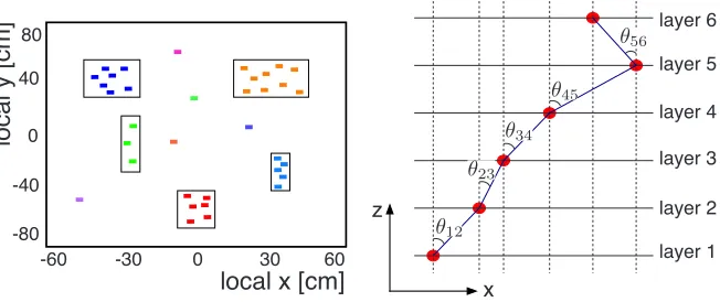
3.1 Spanning Tree (ST) algorithm
The Spanning Tree algorithm was used in the CMS software during the 7 and 8 TeV
run-ning and part of the 13 TeV runrun-ning of LHC. It is based on pattern recognition using all hit
combinations within a chamber. In the first step of the algorithm (
pre-clustering
), hits are
grouped based on their (
x
,
y
) coordinates via the ”box” algorithm, as illustrated in Figure 4
(left), to form groups clearly separated from one another. In the
segment finding
step, each
group of pre-clustered hits is fed to a ”spanning tree” pattern recognition algorithm to check
all combinations of hits within the group and find those that are most consistent with straight
lines. The best segment candidates are chosen using variables sensitive to the angular o
ff
sets
between the lines connecting hits from neighboring layers, as shown in Figure 4 (right), and
minimizing the parameter
A
, which characterizes the spread of the hits, defined as (for an
example case of 6 layers with hits):
A
=
|
θ
12
−
θ
23
|
+
|
θ
23
−
θ
34
|
+
|
θ
34
−
θ
45
|
+
|
θ
45
−
θ
56
|
(2)
The segment candidates chosen via the pattern recognition algorithm are fitted to a straight
line using a least-squares method. The final step of the algorithm (
hit pruning
) aims to
im-prove the segment quality by checking if the removal of any single hit significantly imim-proves
the fit.
local x [cm]
local y [cm]
0
30
60
-30
-60
0
-40
-80
80
40
4.1 Segment Candidate Classification
The best segments are defined as those with the smallest value of a parameter, A, defined as follows (for the case
of a segment candidate containing hits on all six chamber layers):
A
=
|
✓
12
−
✓
23
|
+
|
✓
23
−
✓
34
|
+
|
✓
34
−
✓
45
|
+
|
✓
45
−
✓
56
|
(1)
Figure 1: Definition of distances and angles for the sorting criterion in the spanning tree approach.
The angles in equation 1 are illustrated in fig. 1. These angles are defined in the local x-z plane (the
local-x direction is approlocal-ximately perpendicular to the strips, for which the hit position resolution is highest). For
simplicity, advantage is taken of the fact that
tan(✓
12
)
⇡
✓
12
(2)
for small angles which will be the case for tracks that are nearly orthogonal to the face (local x-y plane) of the
chamber. This condition will hold for tracks that originate at the interaction region of the detector. Using this
approximation, one can write
✓
12
⇠
x
12
d
12
(3)
which greatly simplifies the calculation of A for each segment candidate to the following:
A
=
x
12
d
12
−
x
23
d
23
+
x
23
d
23
−
x
34
d
34
+
x
34
d
34
−
x
45
d
45
+
x
45
d
45
−
x
56
d
56
(4)
If there are no hits on one or more chamber layers within a pre-clustered group, the missing layers are skipped,
resulting in a reduction in the total number of terms contributing to the sum that defines A. For example, if a
pre-clustered group contains hits on five of the six chamber layers, the total number of terms in the sum is reduced
3
✓
12
✓
23
✓
34
✓
45
✓
56
layer 1
layer 2
layer 3
layer 4
layer 5
layer 6
x
z
Figure 4.
Illustration of the Spanning Tree algorithm. Left: Pre-clustering step. Right: Definition of
the angles used for sorting criteria.
3.2 Road Usage (RU) algorithm
5
3.1 Spanning Tree (ST) algorithm
The Spanning Tree algorithm was used in the CMS software during the 7 and 8 TeV
run-ning and part of the 13 TeV runrun-ning of LHC. It is based on pattern recognition using all hit
combinations within a chamber. In the first step of the algorithm (
pre-clustering
), hits are
grouped based on their (
x
,
y
) coordinates via the ”box” algorithm, as illustrated in Figure 4
(left), to form groups clearly separated from one another. In the
segment finding
step, each
group of pre-clustered hits is fed to a ”spanning tree” pattern recognition algorithm to check
all combinations of hits within the group and find those that are most consistent with straight
lines. The best segment candidates are chosen using variables sensitive to the angular o
ff
sets
between the lines connecting hits from neighboring layers, as shown in Figure 4 (right), and
minimizing the parameter
A
, which characterizes the spread of the hits, defined as (for an
example case of 6 layers with hits):
A
=
|
θ
12
−
θ
23
|
+
|
θ
23
−
θ
34
|
+
|
θ
34
−
θ
45
|
+
|
θ
45
−
θ
56
|
(2)
The segment candidates chosen via the pattern recognition algorithm are fitted to a straight
line using a least-squares method. The final step of the algorithm (
hit pruning
) aims to
im-prove the segment quality by checking if the removal of any single hit significantly imim-proves
the fit.
local x [cm]
local y [cm]
0
30
60
-30
-60
0
-40
-80
80
40
4.1 Segment Candidate Classification
The best segments are defined as those with the smallest value of a parameter, A, defined as follows (for the case
of a segment candidate containing hits on all six chamber layers):
A
=
|
✓
12
−
✓
23
|
+
|
✓
23
−
✓
34
|
+
|
✓
34
−
✓
45
|
+
|
✓
45
−
✓
56
|
(1)
Figure 1: Definition of distances and angles for the sorting criterion in the spanning tree approach.
The angles in equation 1 are illustrated in fig. 1. These angles are defined in the local x-z plane (the
local-x direction is approlocal-ximately perpendicular to the strips, for which the hit position resolution is highest). For
simplicity, advantage is taken of the fact that
tan(✓
12
)
⇡
✓
12
(2)
for small angles which will be the case for tracks that are nearly orthogonal to the face (local x-y plane) of the
chamber. This condition will hold for tracks that originate at the interaction region of the detector. Using this
approximation, one can write
✓
12
⇠
x
12
d
12
(3)
which greatly simplifies the calculation of A for each segment candidate to the following:
A
=
x
12
d
12
−
x
23
d
23
+
x
23
d
23
−
x
34
d
34
+
x
34
d
34
−
x
45
d
45
+
x
45
d
45
−
x
56
d
56
(4)
If there are no hits on one or more chamber layers within a pre-clustered group, the missing layers are skipped,
resulting in a reduction in the total number of terms contributing to the sum that defines A. For example, if a
pre-clustered group contains hits on five of the six chamber layers, the total number of terms in the sum is reduced
3
✓
12
✓
23
✓
34
✓
45
✓
56
layer 1
layer 2
layer 3
layer 4
layer 5
layer 6
x
z
Figure 4.
Illustration of the Spanning Tree algorithm. Left: Pre-clustering step. Right: Definition of
the angles used for sorting criteria.
3.2 Road Usage (RU) algorithm
Beginning in 2017, a new segment reconstruction algorithm is used in the CMS software. The
Road Usage algorithm [5] is faster and less complex than ST, and provides better performance
at high luminosity where there is a large number (
∼
35) of background interactions per beam
crossing (pileup). The concept of the algorithm is schematically illustrated in Figure 5. First,
the chamber layers with hits that are closest to and furthest from the CMS interaction point
(shown in red) are taken as base layers. A pair of hits from the base layers is chosen such that
the line connecting the two hits (shown in dashed magenta) points towards the interaction
point. This requirement is an essential distinction with respect to the ST algorithm, and
contributes to the reduction of fake segments with random orientation that are built out of
background hits. Hits from the inner layers that are close to the ”base road” (region shown in
shaded blue) along the line connecting the base hits are added to the segment. If more than
1 hit in a layer satisfies the criteria, separate segments are built for each. After all possible
segments consistent with the base layers are built, those that have common hits are grouped
together. Each segment is fitted to a straight line. From each group only the segment with
the lowest
χ
2
is chosen. If the segment does not pass a certain
χ
2
threshold, the hit furthest
from the fit line is removed in order to minimize the sum of hit residuals, and the segment is
refitted.
z
IP
Figure 5.
Schematic illustration of the Road Usage algorithm.
4 Performance
The performance of the local reconstruction algorithms is quantified in terms of e
ffi
ciency
and resolution, and has been studied with cosmic rays, collision data from LHC, and Monte
Carlo simulated data [1, 6, 7].
4.1 Efficiency to find and associate a rechit to a segment
The e
ffi
ciency to find and associate a rechit to a segment is studied with simulated data.
Rechits that are close to simulated hits in (
R
−
φ
) coordinates are selected. If more than one
rechit is found in a layer, the closest one to the simulated hit is used. The e
ffi
ciency is then
defined as
e
ffi
ciency
=
#hits in segment
#hits in chamber
(3)
As can be seen in Figure 6, the RU algorithm outperforms ST by a few percent for all chamber
types, and the overall e
ffi
ciency is close to 100%.
4.2 CSC spatial resolution
For the measurement of the CSC spatial resolution, a data sample enriched in
Z
→
µ
+
µ
−
events is used, and segments associated with reconstructed muons are selected. For each
segment, one hit is dropped for a specific layer, the segment is refitted, and the residual for
this hit is calculated. This is repeated for each layer, calculating a residual for each case.
These residuals are combined to obtain the spatial resolution for each chamber. Resolution in
the range of 40-150
µ
m is measured, depending on the chamber type (Figure 6, right), which
is well within the CSC design specifications. The di
ff
erence in the resolution per chamber
6
0
20
40
60
80
100
120
140
160
0
1
2
3
4
5
6
7
8
9
10
11
2017
2018
CSC resolution
σ per station (
μm)
chamber type
ME1/1a ME1/1b ME1/2 ME1/3 ME2/1
ME2/2 ME3/1
ME3/2 ME4/1
ME4/2
CMS
Preliminary
CSC Spatial Resolution
(5 fb
-1
)
(11 fb
-1
)
pp 13 TeV
Figure 6.
Left: Hit reconstruction and association e
ffi
ciency. Right: Spatial resolution for the di
ff
erent
CSC types.
4.3 Segment reconstruction efficiency
The e
ffi
ciency to reconstruct a segment is measured using the Tag & Probe technique in a data
sample enriched in
Z
→
µ
+
µ
−
events. The tag is defined as a well-measured muon, the probe
is a track reconstructed in the CMS tracking system and the invariant mass of the tag
+
probe
is consistent with the
Z
boson mass. The probe is projected into the CSC system and a
matching segment is searched for in each CSC the track traverses. The measured e
ffi
ciencies
to reconstruct segments with the RU algorithm are shown in Figure 7 and are generally above
90-95%. A few chambers out of 540 are known to be ine
ffi
cient due to failed electronics
boards.
0
10
20
30
40
50
60
70
80
90
100
67.9 93.5 95.9 97.0 95.8 95.6 97.3 73.5 95.2 95.5 92.3 97.7 97.1 88.9 96.2 95.3 95.4 96.9 96.2 97.2 0.0 96.6 96.5 95.9 96.4 94.6 95.8 97.7 96.1 95.5 98.0 97.2 95.0 83.2 96.5 96.2 78.1 99.3 96.3 98.6 98.6 99.3 98.5 97.7 98.0 97.9 85.2 98.8 99.5 98.6 80.7 98.4 99.1 96.8 96.7 97.7 97.7 97.8 95.6 95.0 96.8 95.9 94.5 95.2 96.1 97.7 95.4 97.5 97.7 96.8 97.0 98.0 96.3 97.8 96.6 97.5 95.1 96.1 94.9 96.1 97.1 97.7 96.7 97.6 97.5 95.3 96.6 97.9 95.2 97.0 97.8 99.1 99.0 98.7 99.4 98.3 98.4 99.0 75.9 99.4 98.6 98.9 78.8 98.8 99.1 99.0 98.8 87.0 73.0 96.1 72.6 96.9 96.6 97.7 96.7 96.9 98.5 96.5 96.1 96.8 96.7 96.3 97.1 93.8 95.7 97.3 95.0 90.3 97.2 93.4 96.8 95.5 97.1 97.0 82.8 96.7 96.1 96.9 95.5 97.9 97.1 97.1 96.0 96.8 98.7 98.8 0.0 97.8 97.0 98.6 98.4 91.8 65.7 87.3 98.0 97.9 98.3 99.3 98.6 98.6 66.3 99.5 90.4 90.2 92.2 92.0 92.0 90.0 94.8 95.1 89.0 93.0 89.5 95.3 91.4 96.7 98.4 93.3 88.0 92.9 90.7 89.5 91.1 79.2 92.0 90.7 82.8 94.3 92.0 100.0 95.3 96.5 89.8 92.3 94.5 88.9 92.4 93.3 96.1 96.8 97.0 97.4 98.8 96.9 95.2 95.2 95.9 97.6 95.7 95.6 96.6 96.7 97.7 97.0 95.1 96.6 94.5 97.3 92.0 97.1 95.3 96.6 95.6 96.7 94.5 94.3 97.4 96.4 96.4 97.3 83.8 94.7 96.7 94.1 94.6 95.7 76.6 96.2 96.0 92.8 95.9 95.1 94.4 95.5 95.7 92.5 94.7 96.9 95.9 95.8 94.6 97.2 95.8 94.2 93.4 93.6 95.1 96.5 92.7 95.1 94.5 96.2 92.9 93.7 96.8 95.2 94.9 0.0 0.0 96.3 92.3 95.1 77.6 93.1 92.8 89.7 85.3 89.9 91.5 90.1 89.9 93.4 93.2 93.8 93.9 89.7 91.7 96.2 87.2 94.8 93.0 92.8 95.2 95.8 93.1 91.0 87.7 94.5 86.6 96.1 93.3 94.8 95.0 0.0 0.0 94.0 95.7 95.0 90.4 90.2 90.4 90.9 88.8 91.2 89.1 93.1 94.1 91.7 92.4 93.1 90.8 91.8 87.6 90.7 90.1 94.3 94.7 92.3 91.1 92.2 92.0 91.3 93.7 90.2 86.5 97.5 89.6 95.7 83.2 92.0 91.4 95.4 95.7 94.7 96.6 95.4 94.9 94.0 95.2 95.8 95.1 94.4 93.3 96.5 96.2 95.3 95.5 95.8 95.3 95.5 93.6 95.0 95.5 94.9 94.0 93.5 94.1 95.3 96.0 94.4 95.6 96.0 92.8 92.2 83.4 95.2 94.7 95.7 89.1 97.4 94.7 96.9 98.1 94.9 95.2 97.1 97.5 95.9 98.2 97.0 80.1 96.2 95.7 96.1 96.5 93.3 95.6 96.7 63.8 96.2 97.5 96.4 96.2 95.9 98.5 97.9 97.0 93.8 83.2 98.0 94.9 96.2 97.7 95.6 91.1 88.9 93.3 90.5 88.1 97.9 93.8 93.4 91.5 92.6 64.3 87.5 93.5 90.0 86.9 69.3 94.7 90.1 96.5 93.0 98.2 88.8 89.6 90.3 93.3 90.8 90.2 93.2 87.8 92.3 99.3 86.8 91.3 91.0 89.8 96.4 84.9 98.4 75.8 97.7 98.6 98.9 98.6 98.8 98.5 99.5 98.2 97.7 98.4 98.9 99.3 99.0 98.6 98.8 96.1 96.4 96.0 96.1 83.5 96.6 96.4 97.3 96.5 96.8 95.5 95.4 97.4 97.1 85.9 96.2 96.1 94.9 81.7 96.6 94.8 97.2 98.4 95.3 96.7 96.4 95.1 96.4 94.5 97.4 97.3 94.7 97.4 95.7 97.3 96.9
98.8 97.5 99.4 98.5 98.8 98.0 73.2 99.0 96.7 99.1 98.9 95.0 99.3 98.3 99.9 98.4 99.2 99.8 96.5 96.8 96.5 96.8 95.3 97.7 95.0 97.0 97.3 98.4 96.1 97.0 97.3 95.1 96.5 96.5 95.7 97.5 78.2 96.1 96.6 97.7 96.9 95.8 95.4 96.3 95.8 96.4 78.1 97.5 97.3 96.2 97.2 96.8 95.6 95.9 99.5 97.3 99.0 99.5 99.2 99.2 98.8 100.0 98.6 98.9 96.9 98.0 99.6 99.4 82.6 98.2 98.7 98.7 94.8 97.9 94.8 96.1 96.6 97.5 94.3 96.7 95.9 96.7 95.0 96.1 95.2 95.2 96.2 97.4 94.9 97.4 97.4 96.8 96.4 96.9 98.0 97.0 95.7 95.7 96.4 97.1 95.1 94.4 94.7 81.9 97.2 96.5 97.0 96.9
CSC Segment Reconstruction Efficiency (%)
φ
0
π
/2
π
3
π
/2
2
π
Endcap/Station/Ring
ME-42
ME-41
ME-32
ME-31
ME-22
ME-21
ME-13
ME-12
ME-11B
ME-11A
ME+11A
ME+11B
ME+12
ME+13
ME+21
ME+22
ME+31
ME+32
ME+41
ME+42
=13 TeV
s
CMS Preliminary 2017
2.1 1.2 0.8 0.7 0.7 1.0 0.9 1.9 1.0 1.0 1.0 0.7 0.7 1.5 0.8 0.9 0.9 0.8 0.8 0.8 0.0 0.9 0.8 0.8 0.9 0.9 0.8 0.7 0.8 0.8 0.6 0.8 0.9 1.6 0.7 0.8 1.5 0.4 0.6 0.5 0.5 0.5 0.5 0.7 0.6 0.7 1.4 0.7 0.4 0.6 1.4 0.6 0.4 0.6 0.7 0.7 0.7 0.7 0.8 0.9 0.7 0.9 1.1 1.0 0.7 0.7 0.8 0.7 0.7 0.7 1.0 0.0 0.8 0.7 0.9 0.8 1.0 0.8 0.9 0.8 0.8 0.6 0.7 0.7 0.8 0.8 0.8 0.8 0.8 0.8
0.6 0.5 0.4 0.5 0.3 0.5 0.5 0.6 1.5 0.5 0.5 0.6 1.4 0.5 0.4 0.4 0.4 1.2 2.1 0.9 1.9 0.7 0.7 0.6 0.7 0.9 0.6 0.8 0.1 0.8 0.8 0.8 0.6 1.0 0.8 0.9 5.0 1.3 0.8 1.1 0.7 0.9 0.8 1.0 1.7 0.8 0.9 0.7 0.8 0.8 0.7 0.8 0.8 0.7
0.5 0.5 0.0 0.5 0.6 0.5 0.5 1.0 1.6 1.1 0.6 0.6 0.5 0.4 0.5 0.4 1.4 0.4 3.1 4.2 3.7 4.3 4.9 3.8 3.9 4.3 3.8 4.1 4.7 4.0 3.6 3.3 1.6 4.0 4.2 4.0 4.5 4.2 3.9 4.9 3.6 5.2 6.5 3.7 4.5 0.0 3.8 3.5 4.6 3.7 3.4 4.8 3.8 4.3 1.0 0.9 1.1 0.8 0.5 0.8 1.1 1.0 1.1 0.9 1.0 1.0 1.2 0.9 0.9 0.9 1.6 0.9 1.1 0.8 1.7 0.9 1.2 0.9 1.1 1.1 1.2 1.2 0.8 1.0 1.0 0.0 2.4 1.2 1.2 1.4 1.1 1.0 2.1 1.0 1.0 1.2 0.9 0.8 1.1 0.8 1.0 1.3 1.0 0.9 1.0 1.0 1.2 0.9 1.1 1.1 1.3 1.2 1.1 0.9 1.4 1.1 1.1 1.0 1.2 1.8 0.9 0.8 1.2 0.0 0.0 1.0 2.5 2.0 3.7 2.2 2.7 2.6 3.7 2.0 2.9 1.9 2.6 2.3 1.9 2.6 2.5 3.0 2.1 1.8 3.1 2.2 2.0 2.3 2.4 0.0 2.3 2.3 2.4 2.1 2.5 1.6 2.9 2.0 2.4 0.0 0.0 2.5 2.4 2.0 2.5 2.3 2.7 2.2 2.6 1.8 2.1 2.0 2.6 2.4 2.0 2.3 2.4 1.9 3.1 2.4 2.4 1.9 1.9 2.5 2.5 2.2 1.8 2.4 2.5 2.0 3.1 1.5 2.5 2.1 3.3 2.7 2.6 2.0 1.0 1.1 1.0 1.0 1.1 1.2 1.1 1.0 1.0 0.9 1.1 0.9 0.9 0.9 1.0 0.8 1.2 0.9 1.2 1.1 1.0 1.1 1.2 1.0 1.0 1.0 1.1 1.2 1.1 1.1 1.2 1.3 1.8 1.0 1.1 0.8 1.8 1.0 1.9 1.1 0.9 1.2 1.1 0.8 0.8 1.0 0.6 0.8 2.6 1.2 1.5 0.9 1.0 1.4 1.0 0.9 3.1 0.9 1.1 0.9 1.9 1.0 0.9 0.9 1.1 1.4 2.3 0.9 1.1 1.2 0.9 1.1 4.7 4.0 3.9 3.9 4.7 2.1 4.5 4.2 4.3 3.2 5.5 4.2 3.6 4.0 5.0 5.2 4.1 3.6 3.3 3.9 1.8 4.9 3.6 4.7 4.0 4.4 4.1 3.6 4.1 3.8 0.7 4.2 4.2 4.3 4.8 3.6 1.2 0.5 1.3 0.5 0.5 0.5 0.4 0.5 0.6 0.3 0.5 0.5 0.5 0.5 0.5 0.4 0.5 0.4 0.8 0.7 0.8 0.8 1.8 0.8 0.9 0.7 0.7 0.7 0.9 1.0 0.7 0.7 1.6 0.8 0.9 1.0 1.8 0.7 1.0 0.9 0.6 0.8 1.2 0.7 0.8 0.7 1.0 0.7 0.8 1.1 0.6 0.9 0.6 0.9
0.5 0.5 0.4 0.5 0.5 0.6 1.5 0.5 0.7 0.5 0.4 0.8 0.4 0.6 0.1 0.5 0.4 0.2 0.8 0.8 0.8 0.8 0.9 0.7 0.9 0.8 0.8 0.5 0.7 0.8 0.7 0.9 0.8 0.8 0.9 0.7 1.9 0.8 0.7 0.7 0.8 0.8 0.8 0.9 0.9 0.7 1.9 0.8 0.7 0.9 0.7 0.7 0.9 0.9
0.5 0.6 0.5 0.5 0.5 0.5 0.5 0.0 0.6 0.6 0.5 0.7 0.3 0.5 1.5 0.6 0.5 0.6 1.0 0.7 0.9 0.8 0.7 0.7 1.5 0.7 0.9 0.7 0.9 0.9 1.0 0.8 0.9 0.7 1.0 0.9 0.7 0.8 0.7 0.7 0.7 0.8 1.0 0.8 0.8 0.6 1.1 1.0 0.9 1.9 0.6 0.8 0.8 0.8
2.1 1.3 0.9 0.8 0.8 1.1 0.8 2.0 1.1 1.1 1.1 0.8 0.8 1.6 0.9 1.0 1.0 0.9 0.9 0.9 0.0 1.0 0.9 0.9 1.0 1.0 0.9 0.8 0.9 0.9 0.8 0.9 1.0 1.7 0.8 0.9 1.6 0.5 0.7 0.6 0.5 0.5 0.6 0.8 0.7 0.7 1.4 0.8 0.5 0.6 1.5 0.6 0.5 0.6 0.8 0.8 0.9 0.8 0.9 1.0 0.8 0.8 1.2 1.1 0.8 0.9 0.9 0.8 0.8 0.8 1.1 0.0 1.0 0.8 1.0 0.9 1.0 0.9 1.0 0.9 1.0 0.7 0.8 0.8 0.9 0.9 1.0 0.9 0.9 0.9
0.7 0.6 0.5 0.6 0.4 0.6 0.6 0.7 1.6 0.6 0.6 0.6 1.5 0.6 0.5 0.5 0.4 1.2 2.1 1.1 2.0 0.8 0.8 0.7 0.8 1.0 0.7 0.9 0.1 0.9 0.9 0.9 0.8 1.2 1.0 1.0 1.0 1.4 0.9 1.2 0.8 1.0 0.9 0.9 1.8 1.0 1.0 0.8 1.0 0.9 0.8 0.9 0.9 0.8
0.5 0.5 0.0 0.6 0.6 0.5 0.5 1.0 1.6 1.1 0.6 0.6 0.6 0.5 0.5 0.5 1.5 0.4 3.4 4.4 3.9 4.6 5.3 4.1 4.3 4.5 4.1 4.4 4.9 4.3 3.8 4.3 4.2 4.4 4.5 4.3 4.9 4.4 4.2 5.1 4.0 5.3 6.6 3.9 4.8 3.7 4.2 4.8 4.8 4.0 3.8 5.1 4.2 4.5 1.2 1.1 1.3 1.0 0.7 1.0 1.3 1.2 1.3 1.1 1.2 0.0 1.4 1.1 1.2 1.1 1.8 1.1 1.3 1.0 1.8 1.1 1.5 1.1 1.3 1.3 1.4 1.4 1.0 1.2 1.2 0.0 2.5 1.4 1.4 1.6 1.2 1.1 2.2 1.2 1.1 1.3 1.0 1.0 1.2 1.0 1.1 1.4 1.1 1.0 1.1 1.2 1.3 1.1 1.2 1.3 1.4 1.3 1.2 1.1 1.4 1.2 1.3 1.1 1.3 1.1 1.0 0.9 1.3 0.0 0.0 1.1 2.8 2.3 3.8 2.5 3.0 2.4 4.0 2.3 3.2 2.1 2.8 2.6 2.4 3.0 2.9 3.3 2.6 2.2 3.5 2.5 2.2 2.7 2.9 0.0 2.6 2.6 2.8 2.4 2.8 1.9 3.2 2.2 2.7 0.0 0.0 2.7 2.8 2.3 2.7 2.6 3.0 2.7 3.2 2.0 2.4 2.2 3.0 2.7 2.5 2.5 2.7 2.2 3.5 2.6 2.6 2.2 2.2 2.8 2.9 2.5 2.2 2.6 2.8 2.2 3.3 1.8 2.7 2.3 3.5 3.0 4.6 2.3 1.1 1.2 1.1 1.1 1.2 1.3 1.2 1.1 1.2 1.1 1.2 1.0 1.1 1.0 1.1 0.9 1.4 1.0 1.3 1.2 1.1 1.3 1.3 1.1 1.1 1.0 1.2 1.3 1.2 1.2 1.3 1.5 1.9 1.1 1.2 0.9 1.9 1.2 1.4 1.2 1.1 1.3 1.3 1.0 1.0 1.1 0.8 1.0 2.8 1.4 1.3 1.1 1.2 1.7 1.2 1.1 3.2 0.0 1.3 1.0 1.2 1.2 1.0 1.1 1.3 2.6 2.5 0.9 1.3 1.3 1.1 1.3 5.1 4.2 4.2 4.3 4.9 3.8 4.8 4.6 4.6 3.6 5.6 4.5 3.9 4.3 5.2 5.3 4.4 3.9 3.6 4.2 4.4 5.2 3.9 5.0 4.2 4.8 4.5 4.0 4.4 4.1 3.9 4.6 4.5 4.6 5.0 4.5 1.2 0.5 1.3 0.6 0.6 0.5 0.5 0.5 0.6 0.4 0.5 0.6 0.5 0.5 0.5 0.5 0.5 0.5 0.9 0.8 0.9 0.9 1.9 0.9 1.0 0.0 0.9 0.8 1.0 1.1 0.8 0.8 1.7 0.9 1.0 1.1 1.9 0.8 1.1 1.0 0.7 1.0 0.8 0.9 1.0 0.8 1.1 0.9 0.9 1.2 0.7 1.0 0.8 1.0
0.5 0.5 0.4 0.6 0.5 0.6 1.5 0.5 0.8 0.5 0.5 0.9 0.5 0.6 0.5 0.6 0.5 0.4 0.8 0.9 0.9 0.9 1.0 0.8 1.0 1.0 0.9 0.6 0.8 0.9 0.8 1.0 0.9 0.9 1.1 0.9 2.0 0.9 0.8 0.8 0.8 0.9 0.9 1.0 1.0 0.8 2.0 0.9 0.8 1.0 0.8 0.0 1.0 1.1
0.6 0.7 0.6 0.6 0.6 0.6 0.6 0.2 0.7 0.7 0.6 0.7 0.4 0.6 1.5 0.6 0.6 0.7 1.1 0.8 1.0 0.9 0.8 0.8 1.0 0.8 1.0 0.8 1.0 1.0 1.1 1.0 0.9 0.8 1.1 1.0 0.8 0.9 0.8 0.8 0.8 0.8 1.0 0.9 0.9 0.7 1.1 1.0 1.0 1.9 0.7 0.9 0.9 0.9
![Figure 1. R-z projection of one quadrant of CMS in the global coordinate system of the detector [1].The horizontal axis is parallel to the beam and the interaction point is at the lower left corner.](https://thumb-us.123doks.com/thumbv2/123dok_us/7996438.1327855/2.482.64.425.128.360/figure-projection-quadrant-coordinate-detector-horizontal-parallel-interaction.webp)