Optimization of Cutting Parameters in High Speed Trochoidal
Machining
Tushar Mestry1 and Niyati Raut2 1
Mechanical Department, VIVA Institute of Technology, Virar (E), Maharashtra, India
2
Mechanical Department, VIVA Institute of Technology, Virar (E), Maharashtra, India
Abstract
The aim of this paper is to implement and optimize Trochoidal Machining technique as a part of High Speed Machining in Industries. In this Trochoidal Machining and Taguchi Method of optimization will be used to achieve higher efficiency and good surface finish. In this paper the effect of Process parameters on material removal rate (Q) and surface roughness (Ra) of Mild Steel is been studied. Also we know that surface finish is most important criteria to determine the quality and this surface finish depends on various cutting parameters selected for machining. Thus we require some standard tools and techniques for analyzing parameters and getting best result from it. He experiment is analyzed by Taguchi L9 orthogonal array, Grey Relational Analysis and confirmation is done using Linear Regression. For experimentation the input parameters selected are Spindle Speed (S), Central Feed (Vf), Width of Cut (Ae) and Depth of Cut (Ap) while output parameters investigated are Machining Time (T), Material Removal Rate (Q) and Surface roughness (Ra). For each experiment Surface roughness is tested using Surface roughness tester, Material Removal Rate (Q) is calculated by standard formula and after machining each slots machining time is being recorded.
Keywords: Trochoidal Machining, High Speed Machining, Taguchi Method, L9 orthogonal array ,Grey Relational Analysis, Linear Regression.
1. Introduction
Increasing competition and pressure has lead organization to implement new measures and optimizing the current technology possibly using new technologies, which include High Speed Machining and Trochoidal Machining. With the wide use of CNC machines and CAD/CAM systems superior advantages of rapid manufacturing techniques by using High-Speed Machining (HSM) and Trochoidal Machining has been demonstrated. In addition to increase productivity, HSM is capable to generate burr-free edges high-quality surfaces, virtually a stress free component and it can machine thin-wall work-pieces. Another significant advantage of high speed machining is low heating of machined parts and tool. As we know surface roughness is a quality indicator and also the last stage in controlling the machining performance and the operation cost. Thus selection of optimal cutting parameters is very important
factor to achieve good surface finish. As Trochoidal Machining being a new technique very few companies has implemented it on experimental bases but still it has good scope to be used on daily basis. Thus to implement it practically and make users confident of using it regularly the experiment has been designed.
2. Problem Definition
The products manufactured today by using Press Tools and Moulds require excellent accuracy with good surface finish. This totally depends on type of machining method and type of machining parameters used. Thus precise control of parameters is required to optimize quality in manufacturing. Today Mould and Tool makers are using different variety of materials to manufacture tools and we know each material has different chemical composition with different properties. Thus machining of different material and obtaining higher surface finish is very important. Here is where the problem starts i.e. different material, different parameters and so variation in surface finish.
Now a day’s Industries have short cycle time i.e. They want the machining to be done in short time span maintaining good surface finish. Thus short machining time is another problem which needs optimization. While optimizing the parameters used to obtain surface finish need to be kept same in order to achieve good surface finish. Thus we need to neglect some parameters and find an optimal solution which will lead us to achieve constant surface finish and low machining time on different material.
3. Methodology
The methodology includes implementation of High Speed Machining, Trochoidal Machining, Taguchi Method and Grey Relational Analysis.
3.1 High Speed Machining
"Machining at the Resonant Frequency of the Machine," which goes to HSM techniques for selecting spindle speeds that minimize chatter. HSM requires several different components in order to effectively speed up the roughing process. It starts with High speed tool path. An HSM tool path is one that reaches and maintains very high spindle speeds and feed rates, with a trajectory that is smooth and rounded throughout, no matter what the topology or geometry of the part. The preview of this is shown in Fig. 3.1.
Fig. 3.1 High Speed Machining
3.2 Trochoidal Machining
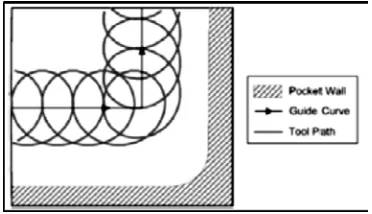
Trochoidal milling is a process where the tool path continuously re-crosses itself as the tool feeds through an outline of constant radius arcs as illustrated in Fig. 3.2. This process uses circular milling and slicing so that the forces on the tool are kept relatively constant. Trochoidal machining is therefore appropriate to use in high speed machining (HSM) as the cutting tool always moves along a curve with a constant radius and this also makes it possible to maintain a relatively consistent feed rate throughout the machining process.
Fig. 3.2 Trochoidal Machining
3.3 Taguchi Methodology
a. System Design: It determines vital design factors and appropriate working levels. In this experiment there are many different parameters available so, we would select
only important factors which will affect our output and will help us to get good results.
b. Parameter Design: Its objective is to conduct experiment and identify optimal design factors to improve performance and reduce variation. As we have designed system we need to select an orthogonal array that will lead to optimal parameter design. Thus by observing the system design we select a standard orthogonal array i.e. L9 (3^4). c. Tolerance Design: Its objective is to determine optimal settings identified during parameter design process. This leads to robust design in which the designed process delivers the target value. Thus after using the experimental data we apply the Taguchi Design and obtain Signal to Noise ratio which helps us to find target value.
3.4 Grey Relational Analysis
Grey relational analysis (GRA), also called Deng's Grey Incidence Analysis model. GRA uses a specific concept of information. It defines situations with no information as black, and those with perfect information as white. However, neither of these idealized situations ever occurs in real world problems. This analysis can be used to represent the grade of correlation between two sequences so that the distance of two factors can be measured discretely. The steps used for GRA are as follows:
a.Data Pre-Processing: It is a process of transferring the original sequence to a comparable sequence. For this purpose the experimental results are normalized in the range between zero and one. The normalization can be done form three different approaches. If the target value of original sequence is infinite, then it has a characteristic of “the larger-the –better”. The original sequence can be normalized as follows.
……..………. (3.1)
Where, Xi*(ki) is the value after the grey relational generation (data pre-processing), Max Xi (k) is the largest value of (k) Xi, Min Xi (k) is the smallest value of (k) Xi and Xn is the desired value.
b.Grey relational coefficient and grey relational grade: Following data pre-processing, a grey relational coefficient is calculated to express the relationship between the ideal and actual normalized experimental results. They grey relational coefficient can be expressed as follows:
Where, ∆oi (k) is the derivation sequence of the reference sequence Xo*(k) and comparability sequence Xi*(k), namely
∆oi (k) = ⋮ Xo^* (k) - Xi^* (k) ⋮ ∆Max = Max ⋮Xo^* (k) - Xi^* (k) ⋮ ∆Min = Min ⋮Xo^* (k) - Xi^* (k) ⋮
ε is distinguishing or identification coefficient ε to [0,1]. ε = 0.5 is generally used.
4. Case Study
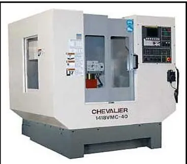
End milling test was conducted on Vertical Machining Centre (CHEVALIER, Model- 1418VMC-40 with Siemens controller).This machine allows high precision positioning. It also allows accurate linear and continuous circular cutting. The achievable spindle speed for the machine is up to 10,000 Rpm as shown in Fig. 4.1.
Fig. 4.1 Vertical Machining Centre
Fig. 4.2 Experimental Setup
4.1 Tooling
The tool used for End Milling process is Solid Carbide End milling cutter with High Helix Flute. The diameter of tool is 8mm, Length is 70mm, flute length 25mm and Helix angle 45 Degrees.
4.2 Material
The work piece material used is Mild steel. Mild steel is also known as plain-carbon steel. The sample of Mild steel is in the form of rectangular blocks, havingsize 150 x 100 x 50 mm. The chemical composition of Mild Steel is shown in Table 4.1
Table 4.1 Chemical Composition Mild Steel
4.3 Experimental Procedure and Analysis
The experiment is designed as per Taguchi Design Approach. This approach starts with following three stages. i. System Design: In this experiment we would select only important factors which will affect our output and will help us to get good results. The Process parameters that are to be selected are shown in Table 5.2.
Table 4.2 System Design for Mild Steel
ii. Parameter Design: Thus by observing the system design we select a Taguchi standard orthogonal array i.e. L9 orthogonal array. According to this array we are going to record data which is shown in Table 4.3.
Chemical
Composition C Si Mn P S
Analysis in % 0.16
0.18 0.40 0.70
0.90 0.040 0.040
Sr. No.
INPUT Parameters
Spindle Speed
(S)
Central Feed
(Vf)
Width of Cut
(Ae)
Depth of Cut
(Ap)
Factors A B C D
1. Level- 1 3581 1504 0.16 8
2. Level- 2 4775 2865 0.20 12
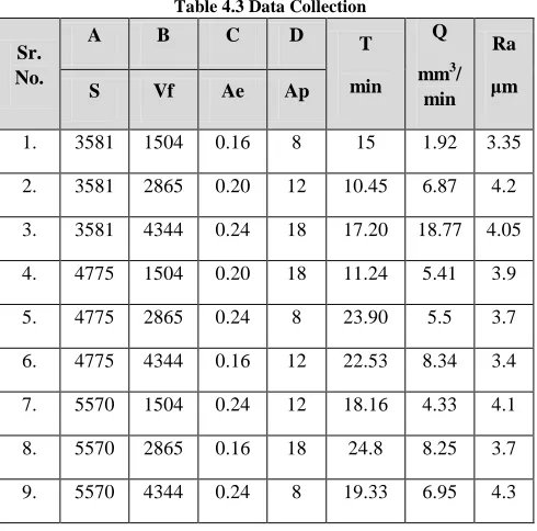
Table 4.3 Data Collection
Sr. No.
A B C D T
min Q
mm3/ min
Ra
μm
S Vf Ae Ap
1. 3581 1504 0.16 8 15 1.92 3.35
2. 3581 2865 0.20 12 10.45 6.87 4.2
3. 3581 4344 0.24 18 17.20 18.77 4.05
4. 4775 1504 0.20 18 11.24 5.41 3.9
5. 4775 2865 0.24 8 23.90 5.5 3.7
6. 4775 4344 0.16 12 22.53 8.34 3.4
7. 5570 1504 0.24 12 18.16 4.33 4.1
8. 5570 2865 0.16 18 24.8 8.25 3.7
9. 5570 4344 0.24 8 19.33 6.95 4.3
iii. Tolerance Design: After using the experimental data we apply Taguchi Design and obtain Signal to Noise ratio which helps us to find target value.
Table 4.4 Experimental Result
Sr. No.
T
min Q
mm3/ min
Ra
μm
S/N
(T)
S/N
(Q)
S/N
(Ra)
1. 15 1.92 3.35 -23.52 5.66 -10.50
2. 10.45 6.87 4.2 -20.38 16.73 -12.46
3. 17.20 18.77 4.05 -24.71 25.46 -12.15
4. 11.24 5.41 3.9 -21.01 14.66 -11.82
5. 23.90 5.5 3.7 -27.56 14.80 -11.36
6. 22.53 8.34 3.4 -27.05 18.42 -10.63
7. 18.16 4.33 4.1 -25.18 12.72 -12.25
8. 24.8 8.25 3.7 -27.88 18.32 -11.36
9. 19.33 6.95 4.3 -25.72 16.83 -12.67
4.4 Results
By implementing Taguchi method for the above experiment we have found optimal values for optimal setting. By using main effect plots relationship between various parameters can be simplified as shown below.
Fig. 4.1 Effects of Process Parameters on Machining Time
Fig. 4.2 S/N Ratio Vs Process Parameters for Machining Time
From Fig. 4.1 and Fig. 4.2 the various effects of process parameters observed are shown below:
a.Effects of Spindle Speed on Machining Time: It is
observe that machining time increases proportionally as spindle speed varies from 3581 to 5570 RPM and machining time increases from 13 min to 21 min. From S/N ratio graph it is observed that values decreases linearly as the spindle speed increases gradually and the given value of S/N ratio lie between -27 to -23.
b.Effects of Central Feed on Machining Time: It observed that as central feed increases from 1504 to 4344 mm/ min, machining time increases from 15 to 20 min. From mean of S/N ratio graph the value lies between 26 to -23.
c.Effects of Width of Cut on Machining Time: It is
observe that as width of cut increases from 0.16 to 0.24 mm the machining time decreases from 21 to 14 min. From mean of S/N ratio graph, the values increases and decreases as width increases from 0.16 to 0.24 mm.
d.Effects of Depth of Cut on Machining Time: It is
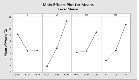
Fig. 4.3 Effects of Process Parameters on Material Removal Rate
Fig. 4.4 S/N Ratio Vs Process Parameters for Material Removal Rate
From Figure 4.3 and Figure 4.4 the various effects of process parameters observed are shown below:
a.Effects of Spindle Speed on Material Removal Rate: It is observed that Material Removal Rate decreases as spindle speed increases from 3581 to 5570 RPM. From S/N ratio graph it is observed that values lie linear as the spindle speed increases gradually and the given value of S/N ratio is at 16.
b.Effects of Central Feed on Material Removal Rate: It is observed that as Material Removal Rate increases from 3 to 12 mm3 /min as central feed increases from 1504 to 4344 mm/min. From mean of S/N ratio graph the value lies between 10 to 20.The values increases linearly as the central feed increases from 1504 to 4344 mm/min. c.Effects of Width of Cut on Material Removal Rate: It is
observe that as width of cut increases from 0.16 to 0.24 mm the Material Removal Rate increases from 6 to 10
mm3 /min. From mean of S/N ratio graph, the values
increases from 14 to 18 as width increases from 0.16 to 0.24 mm.
d. Effects of Depth of Cut on Material Removal
Rate: It is observe that as depth of cut increases from 8 to 18 mm the Material Removal Rate increases from 4 to 11
mm3 /min. From mean of S/N ratio graph, the values
increases linearly from 12 to 20 as depth of cut increases from 8 to 18 mm.
Fig. 4.5 Effects of Process Parameters on Surface Roughness
Fig. 4.6 S/N Ratio Vs Process Parameters for Surface Roughness
From Figure 4.5 and Figure 4.6 the various effects of process parameters observed are shown below:
a.Effects of Spindle Speed on Surface Roughness: It is
observed that Surface Roughness decreases as spindle speed increases from 3581 to 5570 RPM and mean of Surface Roughness increases from 3.6 to 4.1 μm. From S/N ratio graph it is observed that values decreases as the spindle speed increases gradually and the given value of S/N ratio lies from -12 to -11.
b.Effects of Central Feed on Surface Roughness: It
observed that as Surface Roughness increases from 3.8 to 3.9 μm as central feed increases from 1504 to 4344 mm/min. From mean of S/N ratio graph the value lies between -12 to -11.5.The values increases linearly as the central feed increases from 1504 to 4344 mm/min.
c.Effects of Width of Cut on Surface Roughness: It is
observe that as width of cut increases from 0.16 to 0.24 mm the Surface Roughness increases from 3.5 to 4.2 μm. From mean of S/N ratio graph, the values decreases from -11 to -12.5 as width increases from 0.16 to 0.24 mm.
d.Effects of Depth of Cut on Surface Roughness: It is
4.5 Optimization of Parameters by GRA
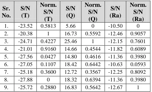
In Grey relational analysis, experimental data are first normalized ranging from zero to one. This process is known as Grey relational generation. Next, based on normalized experimental data, Grey relational coefficient is calculated to represent the correlation between the desired and actual experimental data. Then overall Grey relational grade is determined by averaging the Grey relational coefficient corresponding to selected responses. The overall performance characteristic of the multiple response process depends on the calculated Grey relational grade. This approach converts a multiple response process optimization problem into a single response optimization. The optimal parametric combination is then evaluated which would result highest Grey relational grade. The GRA evaluation is shown below in Table 4.5 and Table 4.6.
Table 4.5 S/N Ratios and Normalized S/N Ratios
Sr. No. S/N (T) Norm. S/N (T) S/N (Q) Norm. S/N (Q) S/N (Ra) Norm. S/N (Ra)
1. -23.52 0.5813 5.66 0 -10.50 0 2. -20.38 1 16.73 0.5592 -12.46 0.9057 3. -24.71 0.4227 25.46 1 -12.15 0.7601 4. -21.01 0.9160 14.66 0.4544 -11.82 0.6089 5. -27.56 0.0427 14.80 0.4616 -11.36 0.3980 6. -27.05 0.1107 18.42 0.6442 -10.63 0.0593 7. -25.18 0.3600 12.72 0.3567 -12.25 0.8092 8. -27.88 0 18.32 0.6394 -11.36 0.3980 9. -25.72 0.2880 16.83 0.5642 -12.67 1
Table 4.6 Grey Relational Coefficient & Grade
Sr. No. GRA Coefficient (T) GRA Coefficient (Q) GRA Coefficient (Ra) Grade
1. 0.5443 0.3333 0.3333 0.4036 2. 1 0.5314 0.8414 0.7909 3. 0.4641 1 0.6757 0.7133 4. 0.8562 0.4782 0.5611 0.6318 5. 0.3431 0.4815 0.4537 0.4261 6. 0.3599 0.5842 0.3471 0.4304 7. 0.4386 0.4373 0.7238 0.5332 8. 0.3333 0.5810 0.4537 0.4560 9. 0.4125 0.5343 1 0.6490
The experiment having best performance can be viewed from highest Grey Relational Grade. But for further simplification we need to build response table for Grey Relational Grade to study its effect. For this we will average the Grey Relational Grade in following sequence
i.e. Experiment 1 to 3, 4 to 6 and 7 to 9. This will help us to study Main effect on machining parameters. The main effect is calculated by subtracting higher value to lower value for those parameters. The Response table for Grey Relational Grade is shown in Table 4.7. This table indicates total mean of Grey Relational Grade for nine experiments. In this larger the grey relational grade, the better is the multiple performance characteristics. However, the relative importance of the performance characteristics still needs to be known, so that the optimal combinations of the machining parameter levels can be determined more accurately.
Table 4.7 Response for Grey Relational Grade
Symb. M/C
Parameter
Grey Relational
Grade Main
Effect Rank
Level 1 Level 2 Level 3
A Spindle Speed (S) 0.636 0* 0.496 1 0.546
1 0.1398 2
B Central Feed (Vf) 0.522 9 0.557 7 0.597
5* 0.0746 4
C Width of Cut (Ae) 0.533 2 0.690 6* 0.557
5 0.1573 1
D Depth of Cut (Ap) 0.492 9 0.584 9 0.600
4* 0.1075 3
From Table 4.7, the optimal parameter combination was determined as A1 (Spindle Speed)-B3 (Central Feed)-C2 (Width of Cut)-D3 (Depth of Cut) shown by *.
4.6 Confirmation Test
The purpose of this confirmation test is to validate the conclusions drawn during the analysis phase. By using Regression equation we predict the optimal Machining Time, Material Removal Rate and Surface Roughness. The Regression equation obtained by using Minitab software is shown below:
Machining Time (T) = 4.9 + 0.00356 S + 0.00184 Vf - 31.3 Ae - 0.182 Ap
Material Removal Rate (Q) = -8.35 - 0.001664 S + 0.002449 Vf + 39.1 Ae + 0.659 Ap
Surface Roughness (Ra) = 2.095 + 0.000022 S + 0.000014 Vf + 6.84 Ae + 0.0174 Ap
Table 4.8 Confirmation Results
Sr. No
.
Response Predicted Error
T Q Ra T Q Ra T Q Ra
1. 16.
07 15. 63 3.8 6 16. 11 16. 01 3.7 6 0.0 4 0.3
A confirmatory experiment was performed using the optimum values and it was found that experimental response values were close enough to predicted values. The values and percentage error between actual and predicted values of the responses are given in Table 4.8. The percentage error between the actual and predicted values of the responses falls below 5%, which shows that the optimized value of Trochoidal machining process parameters obtained is good enough for achieving the target set during the experiment.
By using Taguchi’s L9 orthogonal array and Grey relational analysis the multi response characteristics such as Machining Time (T), Material Removal Rate (Q) and Surface Roughness (Ra) were optimized. The optimal parameter combination obtained were, A1 (Spindle Speed)-B3 (Central Feed)-C2 (Width of Cut)-D3 (Depth of Cut) having an output Machining Time 16.07 Min.,
Material Removal Rate 15.63 mm3 /min and Surface
Roughness as 3.86 Microns.
5. Conclusion
The literature presented in this paper describes in brief of High Speed Trochoidal Machining. This method of programming can be used on all type of CNC Milling machines. In High Speed Trochoidal Machining full flute length of cutter is used to increase material removal rate. This leads to reduce machining time, tool wear and obtain good surface finish. Thus implementation of this method leads to many different benefits to company. The case study presented in this paper helps us to understand and implement High Speed Machining practically. By experimenting and analyzing it using Taguchi method Trochoidal machining process parameters obtained are good enough to achieving the target set during the experiment.
Acknowledgments
The authors would like to express his deep gratitude to Mr. Dinesh Kapoor proprietor of VDA Technologies for Machining Support, Dr. Arun Kumar, Asst. Prof. Niyati Raut, Asst. Prof. Nilesh Nagare and all other authors for their guidance on such a good topic
References
[1] M.Salehia, M.Bluma, B.Fath, T.Akyolb, R.Haasa, J. Ovtcharovac, Epicycloidal versus trochoidal milling- Comparison of cutting force, tool tip vibration, and machining cycle time, CIRP Conference on High Performance Cutting, 46 , 2016, pp.230- 233.
[2] Abram Pleta and Laine Mears, Cutting Force Investigation of Trochoidal Milling in Nickel-Based Superalloy, Procedia Manufacturing, Volume 5, 2016, PP. 1348- 1356.
[3] Mr.Vinit Raut, Mrs. Meeta Gandhi, Mr. Nilesh Nagare, Mr. Aniket Deshmukh, Application of Taguchi Grey Relational Analysis to optimize the process parameters in wire electrical discharge machine, IJISET - International Journal of Innovative Science, Engineering & Technology, Vol. 3 Issue 7, July 2016, pp. 108-115.
[3] Prasad Patil1, Ashwin Polishetty, Moshe Goldberg1, Guy Littlefair and Junior Nomani, Slot Machining Of Ti6al4v With Trochoidal Milling Technique, Journal of Machine Engineering, Vol. 14, No. 4, 2014, pp.42-53.
[4] Vikas Pare1, Geeta Agnihotri, C.M. Krishna, Optimization Of Machining Parameters In High Speed End Milling Of Al-Sic Using Graviational Search Algorithm. International Journal of Recent Advances In Mechanical Engineering (Ijmech), Volume 2, Issue 4, November 2013, pp.45-51. [5] I. Szaloki1, S. Csuka1, S. Csesznok, S. Sipos dr., Can
Trochoidal Milling Be Ideal?, International GTE Conference Manufacturing, November 2012, pp.1-10.
[6] Baohai Wu1, Chengyu Zheng1, Ming Luo1 and Xiaodong He1, Investigation of Trochoidal Milling Nickel-based Superalloy, Materials Science Forum, Vol. 723, June 2012, pp. 332-336.
[7] Barrado E, Vega M, Grande P, Del Valle DL., Optimization of a purification method for metal-containing waste water by using of a Taguchi experimental design, Water Res. 30 (1996) 2309-2314.
[8] Taguchi G, Konishi S., "Taguchi Methods: Orthogonal array and Linear graphs", American Supplier Institute, USA, (1987).
First Author: I am currently in my final year of Masters of Engineering
in Mechanical Engineering (Manufacturing Systems Engineering) at
VIVA Institute of Technology. I have completed my Bachelor of Engineering in Production from Mumbai University and Diploma in Mechanical from Maharashtra State Board of Technical Education. I currently work as Assistant Professor in VIVA Institute of Technology.