A NEW WINDOW FUNCTION FOR FIR FILTER DESIGN AND SPECTRAL ANALYSIS

184 | P a g e

A NEW WINDOW FUNCTION FOR FIR FILTER

DESIGN AND SPECTRAL ANALYSIS

Amit Kumar Patil

H.O.D., EC Department, TSEC Burhanpur, (India)

ABSTRACT

A new window function is presented which like the well known Hamming window offers a preferred property for

use in signal spectrum analysis: the sum of window coefficients with its shifted version by half of the order is

constant for the overlapped region in the time domain. In high orders, the new window has main-lobe width

equal to Hamming window. For low orders, the window parameters are modified to have smaller main-lobe

width compared to Hamming window, while maintaining smaller maximum side-lobe peak. The results indicate

performance improvement of the proposed window compared to Kaiser and Gaussian windows.The FIR filters

designed by windowing method show the efficiency of the new window.

Keywords: FIR, Gaussian, Kaiser, Proposed, Window

I.INTRODUCTION

Window functions are widely used in digital signal processing for the applications in signal analysis and

estimation, digital filter design and signal processing. FFT windows reduce the effects of leakage but can not

only eliminate leakage entirely. In effect, they only change the shape of the leakage. In addition each type of

window affects the spectrum in a slightly different way. Many different windows have been proposed over time

each with its own advantage and disadvantage relative to the others. Some are effective for specific types of

signal types such as random or sinusoidal. Some improve the frequency resolution, that is, they make it easier to

detect the exact frequency of a peak in the spectrum. Some improve the amplitude accuracy that is they most

accurately indicate the level of the peak. The best type of window should be chosen for each specific

application.

Two main applications of the windows in digital signal processing are: data analysis based on Fast Fourier

Transform (FFT) and design of Finite Impulse Response filters from Infinite Impulse Response filters. For FFT

analysis, windows are employed to suppress the so called “leakage effect”, and for FIR filter design according to

the “windowing method”, Gibbs oscillations are attenuated. Desirable characteristics for a window in the

frequency domain are small main-lobe width and side-lobe peak (high attenuation). However, these two

requirements are contradictory, since for a given length, a window with a narrow main-lobe has a poor

185 | P a g e

window order) would be constant:

w [n] + w [n- M/2] = constant, M/2 ≤ n ≤ M (1)

In this paper, a new window function is presented which can be considered as a special case of the important

class of windows, named raised cosine windows. The proposed window has 2~4 dB more side-lobe attenuation

than that of Hamming window, while offering approximately the same main-lobe width and still satisfying the

property in equation (1). The window parameters are modified to avoid the performance degradation for lower

window lengths, which happens for Hamming window.

II.ANALYSIS OF WINDOWING TECHNIQUE

2.1 Types of Windows

There are different types of windows starting from simple type (rectangular window) to more complex type

(Kaiser window). The main goal of these windows is to truncate the impulse response of the filter in order to

generate fixed length filter.

2.1.1 Kaiser window

Syntax: w = kaiser(L,beta)

Description: It returns an L-point Kaiser window in the column vector w. Beta is the Kaiser window β

parameter that affects the sidelobe attenuation of the Fourier transform of the window. The default value for

beta is 0.5. Kaiser window is defined by:

(2)

,

2.1.2 Hamming window

Syntax: w = hamming(L)

Description: It returns an L-point symmetric Hamming window in the column vector w. L should be a positive

integer. The coefficients of a Hamming window are computed from the following equation. Hamming window

is optimized to minimize the maximum side lobe. It is defined by:

186 | P a g e

2.1.3 Gaussian window

Syntax: w = gausswin(N), w = gausswin(N,Alpha)

Description: It returns an N-point Gaussian window in the column vector w. L is a positive integer. The shape

of this window is similar in the frequency domain because the Fourier transform of a Gaussian is also a

Gaussian.

2.1.4 Taylor window

Syntax: w = taylorwin(n)

Description: A Taylor window allows to make tradeoffs between the mainlobe width and sidelobe level. The

Taylor distribution avoids edge discontinuities.Taylor windows are typically used in radar applications, such as

weighting synthetic aperature radar images and antenna design. It returns an n-point Taylor window in a column

vector w. The values in this vector are the window weights or coefficients. n must be a positive integer.

2.1.5 Blackman window

Syntax: w = blackman(L)

Description: It returns the L-point symmetric Blackman window in the column vector w, where L is a positive

integer. Blackman windows have slightly wider central lobes and less sideband leakage than equivalent length

Hamming and Hann windows. Blackman window is defined by:

(4)

2.1.6 Rectangular window

Syntax: w = rectwin(L)

Description: It returns a rectangular window of length L in the column vector w. This function is provided for

completeness; a rectangular window is equivalent to no window at all. It is defined by:

(5)

2.1.7 Hanning window

Syntax: w = hann(L)

Description: It returns an L-point symmetric Hann window in the column vector w. L must be a positive integer.

The coefficients of a Hann window are computed from the following equation.

187 | P a g e

2.2 Windowing Technique

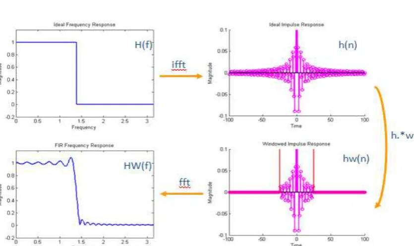
The windowing method involves multiplying the ideal impulse response with a window function to generate a

corresponding filter, which tapers the ideal impulse response. Like the frequency sampling method, the

windowing method produces a filter whose frequency response approximates a desired frequency response. The

windowing method, however, tends to produce better results than the frequency sampling method.

The impulse response of ideal filters is of infinite duration. It is not possible to evaluate the corresponding

frequency response and implement the filter by hardware or software. Thus the impulse response must be

truncated at both ends with respect to the central. Even the impulse response can be truncated when it is small

enough but such a sudden cut off will cause some undesired effects. The window method will reduce them.

In the time domain windowing means to multiply the infinite impulse response hD(n) by a finite duration

window function w(n) to get a truncation. The resulted impulse response h(n) is their product and is given as

follows:

H(n) = hD(n)*w(n) , 0 ≤ n ≤ M (7)

In the window design method we first evaluate the desired filter response hD(n) from the given desired

frequency response HD(



window method. In this method, use is the made of the fact that the frequency response of the filter, HD(



the corresponding impulse response, hd(n) are related by inverse Fourier transform. The subscript D is used to

distinguish between ideal and practical impulse response.

HD(n) =

(

)



 D

H





(8)

The basic idea behind the Window method of filter design is that the ideal frequency response of the desired

filter is equal to 1 for all the pass band frequencies, and equal to 0 for all the stop band frequencies and then the

filter impulse response is obtained by taking the Discrete Fourier Transform (DFT) of the ideal frequency

response. Unfortunately, the filter response would be infinitely long since it has to reproduce the infinitely steep

discontinuities in the ideal frequency response at the band edges. To create a Finite Impulse Response (FIR)

filter, the time domain filter coefficients must be restricted in number by multiplying by a window function of a

finite width. Many windows are used for truncating the signal and the simplest window function is the

188 | P a g e

Fig.1 Windowing Technique

Fig. 2 Spectral Response

III. PROPOSED WINDOW

The goal is to modify Hamming window to lower its maximum side-lobe peak, while holding the main-lobe

189 | P a g e

Hamming window has the shape of

WH[n]= 0.54-0.46 cos(2πn/M), 0 ≤ n ≤ M (9)

This window satisfies the property mentioned in eq. (3), i.e.

WH[ n]+ WH[ n- M/2]= 0.54+0.54, M/2≤n ≤M (10)

On the other hand, Blackman window is composed of three terms as:

WH[n]=0.42-0.5*cos(2πn/M)+0.08*cos(4πn/M), 0 ≤n≤M (11)

that is, it has a DC term, a cosine function with frequency 2/M, and its second harmonic. For this window, due

to the second harmonic, the property in eq.(3) is not satisfied

wH[ n] +wH[ n-M/2]=0.84+0.16*cos(4πn/M ), M/2≤n≤M (12)

However, it can be found that if the third harmonic is added to the Hamming window function, then the property

of eq. (3) will be satisfied. Therefore, the main idea in obtaining the new window is to insert a third harmonic of

cosine function into eq. (1). Thus, an extra degree of freedom is obtained in tuning the window coefficients. In

this way, the proposed window will be as

W[ n]= a0-a1*cos(4πn/M)-a3cos(6πn/M), 0≤n ≤M (13)

Where for normalization, i.e. W[M/2]=1, one have:

a0+a1+a3 = 1 (14)

The new window is also symmetric about point M/2; thus it has a generalized linear phase, like the other

common windows. Checking for the property in eq. (3), one find that

W[n]+W[n-M/2]= 2a0 (15)

Another point of view states that eq. (5) is a four-term raised cosine window, with restriction that the third term

is zero:

W[n]= ∑ ai cos(2iπn/M) 0 ≤ n ≤ M, k = 3, a2 = 0 (16)

The new window can be analyzed in the frequency domain. Its Fourier transform is:

W(ὣ)={a0 D(ω) + a1/2[D(ω - 2π/M) + D(ω + 2π/M)] + a3/2[D(ω -6π/M)+D(ω +6π/M)]}* exp(-jMω/2) (17)

where D(ω) is Dirichlet kernel.

190 | P a g e

algorithm to find the optimal values of the window parameters. For sufficiently large orders, the derived

window is of the form

W[n] = 0.536-0.46cos*(2πn/M)-0.003*cos(6πn/M), 0≤n≤M (19)

Just like Hamming window, the frequency response of the new window is degraded for low orders; therefore

depending on the window order, the above parameters are modified to maintain the efficiency. It shows the

dependence of a0 and a1 on M. It can be easily verified that the coefficients are composed of a monotonic

function and a DC term. Some simple formulas are tried to present the dependence of these parameters on M,

the following formulas approximately fit the data obtained from the optimization:

a0= 0.537 - 0.3/(M+15); a1 = 0.46 + 0.25/(M+15); a3 = 1 - a0 - a1 (20)

IV.RESULTS

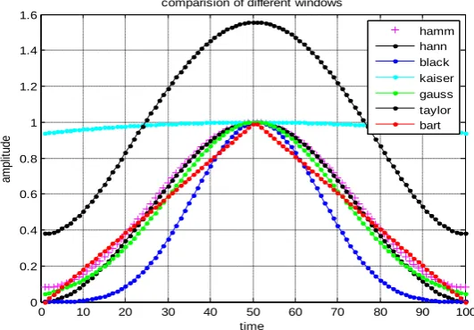
The various methodologies are adopted in developing the programs for proposed window, its comparison with

other windows, performance evaluation, filter designing and plotting their magnitude response, phase response,

pole-zero plot, impulse response, step response, phase delay, group delay and filter information. It discusses the

simulation results for window based FIR filters design.

0 10 20 30 40 50 60 70 80 90 100

0 0.2 0.4 0.6 0.8 1 1.2 1.4 1.6

time

a

m

p

lit

u

d

e

comparision of different windows

hamm hann black kaiser gauss taylor bart

191 | P a g e

0 50 100

0 0.5 1

hamm

0 50 100

0 0.5 1

hann

0 50 100

0 0.5 1

black

0 50 100

0.9 0.95 1

kaiser

0 50 100

0 0.5 1

gauss

0 50 100

0 1 2

taylor

0 50 100

0 0.5 1

bart

0 50 100

0 1 2

rect

0 50 100

0 0.5 1

cheby

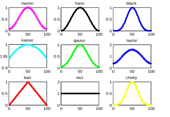
-Fig. 4 Plot of different windows in matrix form

2 4 6 8 10 12 14 16 18 20

0 0.2 0.4 0.6 0.8 1 1.2 1.4 1.6 1.8 2 samples am pl itu de proposed kaiser

Fig. 5 Time-Magnitude response of Kaiser window & Proposed window

0 0.5 1 1.5 2 2.5 3 3.5

-150 -100 -50 0 50 m ag ni tu de proposed

0 0.5 1 1.5 2 2.5 3 3.5

-100 -50 0 50 ksiser m ag ni tu de frequency

192 | P a g e

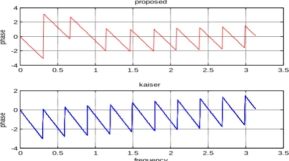
0 0.5 1 1.5 2 2.5 3 3.5

-4 -2 0 2 4 ph as e proposed

0 0.5 1 1.5 2 2.5 3 3.5

-4 -2 0 2 kaiser frequency ph as e

Fig. 7 Frequency-Phase response of Kaiser window & Proposed window

2 4 6 8 10 12 14 16 18 20

0 0.2 0.4 0.6 0.8 1 1.2 1.4 1.6 1.8 2 Samples Am pli tud e Proposed Blackman

Fig. 8 Time-Magnitude response of Blackman window & Proposed window

2 4 6 8 10 12 14 16 18 20 0 0.2 0.4 0.6 0.8 1 1.2 1.4 1.6 1.8 2 Samples Am pli tu de Proposed Gaussian

Fig. 9 Time-Magnitude response of Gaussian window & Proposed window

2 4 6 8 10 12 14 16 18 20 0 0.2 0.4 0.6 0.8 1 1.2 1.4 1.6 1.8 2 Samples Am pli tu de Proposed Taylor

193 | P a g e

V.CONCLUSION

A proposed window is derived for FIR filter designing and spectral analysis which gives better response in

comparison with other windows. Performance evaluation is done in comparison with Hamming, Kaiser and

Gaussian window. Window based FIR filter is designed. Windowing gives good results for proposed window

and it is more convenient. It designs a FIR filter with finite impulse response. It reduces the ripples in the

pass-band and the stop-pass-band due to Gibbs’phenomenon. By choosing the window carefully, various trade-offs can be

managed so as to maximize the filter-design quality in a given application. The window method for digital

filter design is fast, convenient, and robust.

A novel efficient window function has been designed which minimizes the sidelobes. The new window has the

main lobe width less than or equal to that of the Hamming window, while offering less maximum side-lobe

peak. The performance comparison of the proposed window with the other windows showed the better

performance of the proposed window. The average reduction in the side lobe peak of the new window compared

to that of the Hamming, Kaiser, and Gaussian windows is 3 dB, 3.3 dB and 8 dB respectively. The FIR filter

designed with the proposed window achieves less ripple ratio, than those obtained using the windows like

Kaiser, Hamming, Blackman, Gaussian, Hanning, Taylor etc. for all window lengths. The obtained results

indicate that the implemented filter has good performance and stability, and during the implementation of

various cases, it is possible to reach an optimal design used for final design.

REFRENCES

Journal papers:

[1] Mahdi Mottaghi-Kashtiban and Mahrokh G. Shayesteh, “A new window function for signal spectrum

analysis and FIR filter design” in Proc. of IEEE, May 2010.

[2] Abdullah Mohamed Awad, “Adaptive window method for FIR filter design” in Proc. of IEEE, May 2010.

[3] M. G. Shayesteh, M. Mottaghi-Kashtiban, “An efficient window function for design of FIR filters using IIR

filters ,” in Proc. of IEEE Eurocon, pp. 1443-1447, May 2009.

[4] M. G. Shayesteh, M. Mottaghi-Kashtiban, “FIR filter design using a new window function,” in Proc. of

IEEE DSP, July 2009.

[5] K. Avci, N. Nakaroglu, " High Quality Low Order Nonrecursive Digital Filter Design Using Modified

Kaiser Window", IEEE international Conference ,2008.

[6] C. M. Zierhofer, “Data window with tunable side lobe ripple decay”, IEEE Signal Processing Letters, vol.14,

no.11, Nov. 2007.

[7] Rowinska-schwarzweller, M. Wintermantel, “On designing FIR filters using windows based on Gegenbauer

polynomials”, in Proc. IEEE ISCAS, vol. I, pp.413-416, 2002.

[8] M. Jascula, “ New windows family based on modified Legendre polynomials ”, in Proc. IEEE IMTC,

pp. 553-556, 2002.

194 | P a g e

Circuits Syst. II, Analog Digit. Signal Process., vol. 46, no. 1, pp. 40–50, Jan. 1999.

[11] Y.-P. Lin, P. P. Vaidyanathan, “A Kaiser window approach for the design of prototype filters of cosine

modulated filter banks,” IEEE Signal Process. Lett., vol. 5, no. 6, pp. 132–134, Jun. 1998.

[12] I.W. Selesnick, C.S. Burrus,“ Generalized digital Butterworth filter design,” IEEE Trans. Signal Process.,

vol. 46, no. 6, pp. 1688–1694, Jun. 1998.

[13] C. S. Burrus, A. W. Soewito, R. A. Gopinath, “Least squared error FIR filter design with transition bands,”

IEEE Trans. Signal Process., vol. 40, no. 6, pp. 1327–1340, Jun. 1992.

[14] T. Saramaki, A class of window functions with nearly minimum sidelobe energy for designing FIR Filters,

Proc. IEEE Int. Symp. Circuits Syst., Portland, Oregon, pp. 359-362, 1989.

[15] H. Brandenstein, R. Unbehauen, “Least-squares approximation of FIR by IIR filters,” IEEE Trans. Signal

Process., vol. 46, no. 1, pp. 21–30, Jan. 1998.

[16] F. Kaiser, R. W. Schafer, “ On the use of the Io-sinh window for spectrum analysis ” IEEE Trans.

acoustics, Speech, and Signal Processing, vol.28, no.1, pp. 105-107, 1980.

[17] F. J. Harris, “On the use of windows for harmonic analysis with the discrete Fourier transform”, in Proc. Of

IEEE, vol. 66, no. 1, pp. 51- 83, January, 1978.

[18] T. Cooklev, A. Nishihara, “Maximally flat FIR filters,” in Proc. IEEE Int. Symp. Circuits Syst. (ISCAS),

Chicago, IL, May 3–6, 1993, vol. 1, pp. 96–99.

[19] H. J. Orchard, “ The roots of maximally flat-delay polynomials,” IEEE Trans. Circuit Theory, vol. CT-

12, pp. 452–454, Sept. 1965.

Books:

[20] J. Proakis, D. G. Manolakis, Digital Signal Processing, fourth edition, Prentice-Hall, 2007.

[21] Antoniou,” Digital signal processing:”Signal, systems, filters, McGraw-Hill, 2005.

[22] T. S. E1-A1i, Discrete Systems and Digital Signal Processing with MATLAB, CRC Press, 2004.

[23] S. K. Mitra, Digital Signal Processing: A Computer Based Approach, 2nd ed. New York: McGraw Hill,

2002

[24] S.K. Mitra, J.F. Kaiser, Handbook for Digital Signal Process- ing, John Wiley & Sondnc, 1993.

[25] Oppenheim, R. Schafer, J. Buck, Discrete-Time Signal Processing, second edition, Prentice-Hall, 1999.