Two-Phase Flows With Dynamic Contact Angle Effects For Fuel Cell Applications

(1)

University of Windsor University of Windsor

Scholarship at UWindsor

Electronic Theses and Dissertations Theses, Dissertations, and Major Papers

1-24-2019

Two-Phase Flows With Dynamic Contact Angle Effects For Fuel

Cell Applications

Mengcheng Jiang University of Windsor

Follow this and additional works at: https://scholar.uwindsor.ca/etd

Recommended Citation Recommended Citation

Jiang, Mengcheng, "Two-Phase Flows With Dynamic Contact Angle Effects For Fuel Cell Applications" (2019). Electronic Theses and Dissertations. 7640.

https://scholar.uwindsor.ca/etd/7640

This online database contains the full-text of PhD dissertations and Masters’ theses of University of Windsor students from 1954 forward. These documents are made available for personal study and research purposes only, in accordance with the Canadian Copyright Act and the Creative Commons license—CC BY-NC-ND (Attribution, Non-Commercial, No Derivative Works). Under this license, works must always be attributed to the copyright holder (original author), cannot be used for any commercial purposes, and may not be altered. Any other use would require the permission of the copyright holder. Students may inquire about withdrawing their dissertation and/or thesis from this database. For additional inquiries, please contact the repository administrator via email

(2)

TWO-PHASE FLOWS WITH DYNAMIC CONTACT ANGLE EFFECTS FOR FUEL CELL APPLICATIONS

By

Mengcheng Jiang

A Thesis

Submitted to the Faculty of Graduate Studies

through the Department of Mechanical, Automotive & Materials Engineering

in Partial Fulfillment of the Requirements for

the Degree of Master of Applied Science

at the University of Windsor

Windsor, Ontario, Canada

2019

(3)

TWO-PHASE FLOWS WITH DYNAMIC CONTACT ANGLE EFFECTS FOR FUEL CELL APPLICATIONS

by

Mengcheng Jiang

APPROVED BY:

______________________________________________

S. Cheng

Department of Civil and Environmental Engineering

______________________________________________

J. Defoe

Department of Mechanical, Automotive & Materials Engineering

______________________________________________

B. Zhou, Advisor

Department of Mechanical, Automotive & Materials Engineering

(4)

iii

DECLARATION OF CO-AUTHORSHIP / PREVIOUS PUBLICATION

I. Co-Authorship

I hereby declare that this thesis incorporates material that is result of joint research.

Chapter 2 of the thesis (Comparisons and validations of contact angle models) was

co-authored with Dr. Biao Zhou and Xichen Wang. For this paper, Dr. Zhou contributed to

the refinement of main ideas, the follow-up discussions and the revision of the

manuscript. Xichen Wang assisted in the initial numerical model set up. Part of Chapter 3

in this thesis (Numerical Study of Droplet Impact on Inclined Surface: Viscosity Effects)

was co-authored with Dr. Zhou and presented at Fuel Cell Seminar & Energy Exposition

on November 9, 2017 at Long Beach, California.

I am aware of the University of Windsor Senate Policy on Authorship and I certify that I

have properly acknowledged the contribution of other researchers to my thesis, and have

obtained written permission from each of the co-author(s) to include the above

material(s) in my thesis.

I certify that, with the above qualification, this thesis, and the research to which it refers,

is the product of my own work.

II. Previous Publication

This thesis includes two original papers that have been previously published/submitted

for publication in peer reviewed journals/conference proceedings, as follows:

Thesis Chapter Publication title/full citation Publication status

Chapter 2

Jiang M, Zhou B, Wang X. Comparisons and validations of contact angle models.

International Journal of Hydrogen Energy. 2018 Mar 22;43(12):6364-78.

doi: 10.1016/j.ijhydene.2018.02.016

(5)

iv

Chapter 3

(partial)

Jiang M, Zhou B. Numerical Study of Droplet Impact on Inclined Surface: Viscosity Effects. ECS Transactions. 2018 Jan 4;83(1):127-36. doi: 10.1149/08301.0127ecst

Published

I certify that I have obtained a written permission from the copyright owner(s) to include

the above published material(s) in my thesis. I certify that the above material describes

work completed during my registration as a graduate student at the University of

Windsor.

III. General

I declare that, to the best of my knowledge, my thesis does not infringe upon anyone’s

copyright nor violate any proprietary rights and that any ideas, techniques, quotations, or

any other material from the work of other people included in my thesis, published or

otherwise, are fully acknowledged in accordance with the standard referencing practices.

Furthermore, to the extent that I have included copyrighted material that surpasses the

bounds of fair dealing within the meaning of the Canada Copyright Act, I certify that I

have obtained a written permission from the copyright owner(s) to include such

material(s) in my thesis.

I declare that this is a true copy of my thesis, including any final revisions, as approved

by my thesis committee and the Graduate Studies office, and that this thesis has not been

(6)

v ABSTRACT

Liquid water management is still a very critical challenge in the commercialization of

proton exchange membrane fuel cell (PEMFC). Fundamental understanding of two-phase

flow behaviors is of crucial importance to the investigation of water management issues.

Recently, it has been noted that the dynamic contact angle (DCA) plays a critical role in

the two-phase flow simulations and the conventional static contact angle (SCA) model

has obvious limitations in the prediction of droplet behaviors. This thesis mainly focuses

on the numerical modeling and simulation of two-phase flow problems with dynamic

contact angle (DCA) and is presented by four papers. The first paper proposes and

validates an advancing-and-receding DCA (AR-DCA) model that is able to predict both

advancing and receding dynamic contact angles using Hoffman function (Chapter 2). In

the second paper, the AR-DCA model is further applied to simulate droplet behaviors on

inclined surfaces with different impact velocities, impact angles and droplet viscosities

(Chapter 3). The third paper introduces a methodology to improve the evaluation method

of contact line velocity in the AR-DCA model and an improved-AR-DCA (i-AR-DCA)

model is developed (Chapter 4). The last paper presents different flow regimes in a single

(7)

vi

DEDICATION

To my parents, my family and close friends

and

(8)

vii

ACKNOWLEDGEMENTS

I would first like to express my sincerest thanks to my supervisor, Dr. Biao Zhou, for

providing me the opportunity to pursue my Master degree at the University of Windsor

and Clean Powertrain Lab. His guidance, patience and inspiration lead me to the right

direction for my research during my master study. I would also like to express my deep

gratitude to all my committee members, Dr. Jeff Defoe and Dr. Shaohong Cheng, for

their insightful comments and suggestions on my thesis; Dr. Shahpour Alirezaee, for

serving as the chair of my oral defense.

I am also very grateful for Compute Canada and Sharcnet for providing computing

resources which greatly accelerated the simulation progress and made this research

possible. I would also like to acknowledge the support from the Natural Sciences and

Engineering Research Council of Canada (NSERC), the Clean Rail Academic Grant

Program from Transport Canada, and the University of Windsor.

Special appreciation goes to my colleagues in Dr. Zhou’s research group, especially Iman

Azarian Borojeni, and all my close friends in Windsor. Thank you for your

encouragement and companion in these years, which comfort me a lot and help me face

the challenges in my study and life.

Finally, I would like to express my heartfelt gratitude to my family and my parents. Mom

and Dad, thank you for your unconditional love. I would not be able to complete this

(9)

viii

TABLE OF CONTENTS

DECLARATION OF CO-AUTHORSHIP / PREVIOUS PUBLICATION ... iii

ABSTRACT ...v

DEDICATION ... vi

ACKNOWLEDGEMENTS ... vii

LIST OF TABLES ... xi

LIST OF FIGURES ... xii

LIST OF ABBREVIATIONS/SYMBOLS ... xvii

NOMENCLATURE ... xviii

CHAPTER 1 INTRODUCTION ...1

1.1. Proton Exchange Membrane Fuel Cell ... 1

1.2. Water Management and Two-phase Flow in Proton Exchange Membrane Fuel Cells ... 2

1.3. Contact Angle Definition and Dynamic Contact Angle ... 4

1.4. Challenges ... 5

1.5. Objectives and Thesis Overview... 6

References ... 8

CHAPTER 2 COMPARISONS AND VALIDATIONS OF CONTACT ANGLE MODELS ...12

2.1. Introduction ... 12

2.1.1. Dynamic Contact Angle Formulation – Hoffman function ... 12

2.1.2. Numerical Studies on Dynamic Contact Angle ... 14

2.1.3. Summary ... 16

2.2. Fundamental Understanding of Hoffman Function ... 18

2.3. Numerical Methodology ... 19

2.3.1. Governing Equations with Volume of Fluid (VOF) Method ... 20

2.3.2. Implementation of Contact Angle Models ... 21

2.4. Numerical Model Description ... 22

2.4.1. Experiments for Validation ... 22

2.4.2. Computational Domain and Input Parameters ... 23

2.4.3. Mesh Independency ... 25

2.5. Results and Discussion ... 27

(10)

ix

2.5.2. Quantitative Results ... 35

2.6. Conclusions ... 39

Acknowledgements ... 42

References ... 42

CHAPTER 3 DROPLET BEHAVIORS ON INCLINED SURFACES WITH DYNAMIC CONTACT ANGLES ...46

3.3.1. Experiments for Validation ... 49

3.3.2. Computational Domain and Grid Independency ... 51

3.4.1. Effects of Impact Velocity ... 51

3.4.2. Effects of Impact Angle ... 56

3.4.3. Effects of Droplet Viscosity ... 60

References ... 68

CHAPTER 4 IMPROVEMENT AND FURTHER INVESTIGATION ON HOFFMAN-FUNCTION-BASED DYNAMIC CONTACT ANGLE MODEL ...72

4.2.1. Governing Equations and Dynamic Contact Angle ... 75

4.2.2. Modification of the Evaluation Method of Contact Line Velocity ... 75

4.3.1. Computational Domain and Boundary Conditions ... 77

4.3.2. Grid Independency ... 78

4.4.1. Droplet Impact on Inclined Surface ... 80

4.4.2. Liquid Water Behaviors in a Single Straight Microchannel ... 84

References ... 86

CHAPTER 5 NUMERICAL STUDY OF FLOW REGIMES IN MICROCHANNEL WITH DYNAMIC CONTACT ANGLE...90

(11)

x

5.2.2. Governing Equations and Dynamic Contact Angle ... 95

5.2.3. Grid Independency ... 96

5.3.1. Liquid Water Behaviors under Different Water Inlet Flow Rates ... 97

5.3.2. Liquid Water Behaviors under Different Air Inlet Flow Rates ... 102

References ... 106

CHAPTER 6 CONCLUSIONS AND FUTURE WORKS ...110

6.1. Summary and Conclusions ... 110

6.2. Recommendations and Future Works ... 112

APPENDICES ...114

Appendix A ... 114

NUMERICAL SIMULATION OF LIQUID WATER BEHAVIORS IN MICROCHANNEL USING THE MULTI-FLUID VOLUME OF FLUID METHOD ... 114

A.1. Introduction ... 114

A.2. Numerical Model Description ... 117

A.2.1. Computational Domain and Boundary Conditions ... 117

A.2.2. Numerical Methodology ... 118

A.3. Preliminary Results and Discussion ... 121

A.4. Summary and Future Work ... 123

References ... 123

Appendix B ... 128

PERMISSIONS FOR PREVIOUS PUBLISHED WORKS ... 128

(12)

xi

LIST OF TABLES

Table 2.1: Correlations Used in DCA Simulations from Available Literature ... 17

Table 2.2: Detailed Liquid Property, Surface Wettability and Impact Velocity for

Selected Cases ... 23

Table 2.3: Simulation Parameters for Selected Cases ... 24

Table 2.4: Information of Different Grid Resolutions in the Present Study ... 25

Table 3.1 Detailed Liquid Property, Surface Wettability and Impact Velocity for Selected

Cases [15] ... 50

Table 3.2 Calculation Results for the Viscosity of the Glycerin Solution based on Refutas

Equation ... 63

Table 4.1: Information of Different Grid Resolutions for Microchannel Domain ... 79

Table 4.2: Comparison of Numerical Results under Different Grid Resolutions (Re =

49.2, Ca = 0.0023) ... 80

Table 5.1: Comparison of Liquid Water Behavior between the Numerical Simulation

and Experimental Visualization [16] under Ca = 0.011 ... 97

Table 5.2: Simulation Cases under Various Water Inlet Flow Rates with Fixed Air Re

(13)

xii

LIST OF FIGURES

Figure 1.1: Schematic of a PEMFC [3]. ... 2

Figure 1.2: Definition of contact angle. ... 4

Figure 2.1: Dynamic contact angle evolution map. ... 19

Figure 2.2: Schematic of droplet impact on a surface [25]. ... 22

Figure 2.3: (a) Schematic of computational domain used in the numerical simulation; (b) Schematic of the droplet initial and impact position in the computational domain (side-view). ... 24

Figure 2.4: Effects of computational domain size on the numerical results: (a) Case 1; (b) Case 2. ... 25

Figure 2.5: Numerical results of Case 1 under different grid resolution: (a) grid resolution type A; (b) grid resolution type B; (c) grid resolution type C; (d) grid resolution type D. ... 26

Figure 2.6: Numerical results of Case 2 under different grid resolution: (a) grid resolution type A; (b) grid resolution type B; (c) grid resolution type C; (d) grid resolution type D. ... 27

Figure 2.7: Comparison of numerical and experimental results for Case 1 (side-view). (a) Experiment at 0.100, 0.260, 2.020 ms (last three profiles) after impact [34]; (b) A-DCA model (c) AR-DCA model. (d) SCA model. ... 28

Figure 2.8: Comparison of numerical results for Case 1 (3D-view). (a) A-DCA model; (b) AR-DCA model; (c) SCA model. ... 29

Figure 2.9: Comparison of numerical and experimental results for Case 2 (side-view). (a) Experiment [34]; (b) A-DCA model; (c) AR-DCA model; (d) SCA model. 30 Figure 2.10: Comparison of numerical results for Case 2 (3D-view). (a) A-DCA model; (b) AR-DCA model; (c) SCA model. ... 30

Figure 2.11: Comparison of numerical and experimental results for Case 3 (side-view) (a)

(14)

xiii

Figure 2.12: Comparison of numerical results for Case 3 (3D-view) (a) A-DCA model;

(b) AR-DCA model; (c) SCA model. ... 33

Figure 2.13: Comparison of numerical and experimental results for Case 4 (side-view) (a)

Experiment [25]; (b) A-DCA model; (c) AR-DCA model; (d) SCA model. 34

Figure 2.14: Comparison of numerical results for Case 4 (3D-view) (a) A-DCA model;

(b) AR-DCA model; (c) SCA model. ... 34

Figure 2.15: Comparisons of the spreading factor x/D (left column) and dimensionless

droplet spreading length l/D (right column). (a) Case 2; (b) Case 3; (c) Case

4. ... 36

Figure 3.1: Impact of water droplet on smooth glass with α = 10° and different impact

velocities (Left side: experiment from Sikalo [15]; Right side: numerical

results in the present study): (a) We = 50, t =0, 1, 2, 9 ms; (b) We = 161, t =0,

1, 2, 5 ms; (c) We = 391, t =0, 1, 2 ms. ... 52

Figure 3.2: Impact of water droplet on wax with α = 10° and different impact velocities

(Left side: experiment from Sikalo [15]; Right side: numerical results in the

present study): (a) We = 50, t =0, 1, 2, 9 ms; (b) We = 161, t =0, 1, 2, 5 ms;

(c) We = 391, t =0, 1, 2 ms. ... 53

Figure 3.3: Comparison of spreading factor under different impact velocities (We = 50, 161, 391) for water droplet impact on 10° smooth glass: a) simulation and b) experiment [15]. ... 54

Figure 3.4: Comparison of dimensionless spreading length under different impact

velocities (We = 50, 161, 391) for water droplet impact on 10° smooth glass (simulation). ... 54

Figure 3.5: Comparison of spreading factor under different impact velocities (We = 50, 161, 391) for water droplet impact on 10° wax: a) simulation and b) experiment [15]. ... 55

Figure 3.6: Comparison of dimensionless spreading length under different impact

(15)

xiv

Figure 3.7: Impact of water droplet on smooth glass with We = 50 and different impact

angle α (Left side: experiment from Sikalo [15]; Right side: numerical results in the present study): (a) α = 9.5°, t =0, 2, 4, 6, 8 ms; (b) α = 10°, t =0, 1, 2, 9 ms; (c) α = 20°, t =0, 1, 2, 9 ms. ... 57

Figure 3.8: Impact of water droplet on wax with We = 50 and different impact angle α

(Left side: experiment from Sikalo [15]; Right side: numerical results in the

present study): (a) α = 5°, t =0, 2, 4, 6, 8 ms; (b) α = 10°, t =0, 1, 2, 9 ms; (c) α = 20°, t =0, 1, 2, 9 ms. ... 58

Figure 3.9: Comparison of spreading factor under different impact angles (α = 9.5°, 10°, 20°) for water droplet impact on smooth glass with We = 50: a) simulation and b) experiment [15]. ... 59

Figure 3.10: Comparison of dimensionless spreading length different impact angles (α = 9.5°, 10°, 20°) for water droplet impact on smooth glass with We = 50 (simulation). ... 59

Figure 3.11: Comparison of spreading factor under different impact angles (α = 5°, 10°, 20°) for water droplet impact on wax with We = 50: a) simulation and b) experiment [15]. ... 60

Figure 3.12: Comparison of dimensionless spreading length different impact angles (α = 5°, 10°, 20°) for water droplet impact on wax with We = 50 (simulation). ... 60

Figure 3.13: Impact of glycerin droplet onto wax with We = 391: (a) droplet partial

rebound in the experiment [15]; (b) droplet deposition in the experiment [15];

(c) simulation results. ... 61

Figure 3.14: Comparison of numerical results with different viscosities (side-view): a)

µ*; b) 1.5µ*; c) 2µ*; d) 3µ*. ... 64

Figure 3.15: Comparison of numerical results with different viscosities (3D-view): a) µ*;

b) 1.5µ*; c) 2µ*; d) 3µ*. ... 64

Figure 3.16: Comparison of a) spreading factors and b) dimensionless spreading length

(16)

xv

Figure 4.1: Contact angle at the interaction of gas, liquid and solid phases. ... 72

Figure 4.2: Evaluation of contact line velocity in the previous works [15, 16, 20]. ... 74

Figure 4.3: Schematic of contact line velocity evaluation in AR-DCA model (a) and

modification (b). ... 77

Figure 4.4: Schematic of computational domains used in the present study: (a) droplet

impact on inclined surface; (b) liquid water behaviors in a single straight

microchannel. ... 78

Figure 4.5: Schematic of a liquid water slug in microchannel with the length l and height

h. ... 79

Figure 4.6: Comparison of the ratio of water slug length to height (l/h) under different

grid resolution. ... 80

Figure 4.7: Comparison of numerical results for water droplet impact on wax (Case 3 in

Ref. [20]) from AR-DCA and i-AR-DCA models. ... 81

Figure 4.8: Comparison of numerical results for water droplet impact on wax (Case 4 in

Ref. [20]) from AR-DCA and i-AR-DCA models. ... 82

Figure 4.9: Comparison of the spreading factor x/D from AR-DCA and i-AR-DCA

models: (a) water droplet impact on smooth glass (Case 3 in Ref. [20]); (b)

water droplet impact on wax (Case 4 in Ref. [20]). ... 82

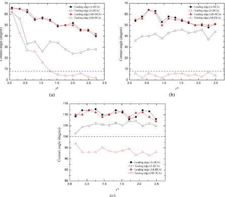
Figure 4.10: Comparison of contact angles at the leading and trailing edges from

AR-DCA and i-AR-AR-DCA models: (a) water droplet impact on smooth glass (Case

3 in Ref. [20]); (b) water droplet impact on wax (Case 4 in Ref. [20]). ... 83

Figure 4.11: Comparison of liquid water evolvement process based on AR-DCA and

i-AR-DCA models (Re= 66.6, Ca = 0.0023). ... 85

Figure 4.12: Comparison of the ratio of water slug length to height (l/h) before

detachment under AR-DCA and i-AR-DCA models. ... 85

(17)

xvi

Figure 5.2: Liquid water evolvement (squeezing flow) at Vair = 10.7 m/s (Re = 66.6) under

various water injection rates: (a) 5 µL/min (Ca = 0.0011); (b) 10 µL/min (Ca

= 0.0023). ... 99

Figure 5.3: Liquid water evolvement (partial-jetting flow) at Vair = 10.7 m/s (Re = 66.6)

and water injection rate 15 µL/min (Ca = 0.0034). ... 100

Figure 5.4: Liquid water evolvement (squeezing flow) at Vair = 10.7 m/s (Re = 66.6) under

various water injection rates: (a) 20 µL/min (Ca = 0.0046); (b) 25 µL/min

(Ca = 0.0057); (c) 30 µL/min (Ca = 0.0069); (d) 50 µL/min (Ca = 0.011). 101

Figure 5.5: Liquid water evolvement under different air inlet velocities at Qwater = 5

µL/min (Ca = 0.0011): (a) Vair = 4.8 m/s (Re = 29.9) (b) Vair = 10.7 m/s (Re =

66.6), (c) Vair = 18.1 m/s (Re = 112.7). ... 103

66.6), (c) Vair = 18.1 m/s (Re = 112.7). ... 104

66.6), (c) Vair = 18.1 m/s (Re = 112.7). ... 105

Figure A.1: Schematic of computational domain for microchannel. ... 118

Figure A.2: Numerical results of liquid water evolvement based on the VOF method (left

column) and the multi-fluid VOF method (right column). ... 122

Figure A.3: Comparison of the ratio of water slug length to height (l/h) before

(18)

xvii

LIST OF ABBREVIATIONS/SYMBOLS

Abbreviations

A-DCA Advancing dynamic contact angle

AR-DCA Advancing-receding dynamic contact angle

CL Catalyst layer

CFD Computational fluid dynamics

DCA Dynamic contact angle

GDL Gas diffusion layer

i-AR-DCA Improved advancing-receding dynamic contact angle

PEMFC Proton exchange membrane fuel cell

SCA Static contact angle

UDF User defined function

VBN Viscosity bending number

VOF Volume of fluid

Greek symbols

𝛼 Inclined angle of surface

𝛾 Surface tension

𝜃 Contact angle

𝜅 Surface curvature

𝜇 Dynamic viscosity

𝜌 Density

(19)

xviii

NOMENCLATURE

Ca Capillary number

Co Courant number

D Initial droplet diameter

d0 Droplet falling distance

F Shift factor

𝑓_Hoff Hoffman function

𝑓_Hoff−1 Inverse of Hoffman function

Hc Height of the microchannel

Lc Length of the microchannel

l Droplet spreading length

Re Reynolds number

S Source term

s Phase volume fraction

t* Dimensionless time for cases of droplet impact on surfaces

ta Dimensionless time for microchannel cases (under same air inlet velocity)

tw Dimensionless time for microchannel cases (under same water inlet velocity)

𝑢⃑ Velocity vector

V0 Droplet initial velocity

Vcl Contact line velocity

Vi Interface velocity

Vp Droplet impact velocity

(20)

xix Subscripts

LG liquid/gas interface

SG Solid/gas interface

SL Solid/liquid interface

a Advancing

cl Contact line

d Dynamic

e Equilibrium

g Gas phase

l Liquid phase

m Momentum

r Receding

(21)

1 CHAPTER 1

INTRODUCTION

1.1.Proton Exchange Membrane Fuel Cell

Fuel cells are energy conversion devices that produce electricity through electrochemical

reaction. Generally, a fuel cell consists of three components: 1) Anode, an electrode

where the oxidation reaction occurs and the electrons are released in the process; 2)

Cathode, an electrode where the reduction reaction occurs and the electrons are

consumed in the process; 3) Electrolyte, a substance that only allows ions to pass through

instead of electrons. One of the remarkable distinctions of fuel cells to the conventional

power sources (batteries, combustion engines) is that fuel cells can be recharged directly

by refueling rather than the time-consuming charging (plugged in) like batteries. Also,

fuel cells are far more efficient and environmentally friendly than combustion engines

[1].

In general, fuel cells can be classified into the following major categories: 1) Proton

exchange membrane or Polymer Electrolyte Membrane fuel cell (PEMFC); 2) Direct

methanol fuel cell (DMFC); 3) Alkaline fuel cell (AFC); 4) Phosphoric acid fuel cell

(PAFC); 5) Molten carbonate fuel cell (MCFC); 6) Solid-oxide fuel cell (SOFC) [2]. In

recent years, PEMFCs have received extensive attentions due to their abilities such as

quick start-up, frequent start-and-stop, low operating temperature, quietness and high

power density. These notable features of PEMFCs make them as one of the most

promising and suitable energy power sources for transportation, portable and stationary

(22)

2

Figure 1.1 shows a schematic of a PEMFC and the basic PEMFC operation process can

be described as follows: on the anode side, hydrogen is delivered as fuel and electrons are

separated from protons (H+) through electrochemical reaction on the catalyst surface;

then the protons will flow through the electrolyte (polymer membrane) to the cathode

side whereas the electrons (e-) will flow though external circuit and generate the

electricity; on the cathode side, the electrons recombine with protons and oxygen to

produce water. The two electrochemical half reactions in a PEMFC are as follows [1]:

Anode side (Oxidation): 𝐻2 ⇌ 2𝐻++ 2𝑒−

Cathode side (Reduction): ½ 𝑂2+ 2𝐻++ 2𝑒−⇌ 𝐻20

Figure 1.1: Schematic of a PEMFC [3].

1.2.Water Management and Two-phase Flow in Proton Exchange Membrane Fuel

Cells

Although PEMFCs have numerous advantages compared to the conventional power

sources, there are still many technical barriers that prevent PEMFCs from

commercialization and broad applicability, mainly in durability, cost and performance

[2]. Water management has significant effects on PEMFC performance and is one of the

most critical challenges in recent research progress. On one hand, liquid water is needed

(23)

3

maintained [4]; on the other hand, excessive water may block the pores of the gas

diffusion layer (GDL) and the catalyst layer (CL) and cause the flooding issues, which

consequently limits the mass transport of reactant. Therefore, it is very important to

maintain a proper balance between membrane humidification and liquid water flooding in

order to optimize PEMFC performance.

Numerical modeling and simulation based on computational fluid dynamics (CFD) are

promising approaches to obtain basic understanding on liquid water behaviors in

PEMFCs, especially in gas flow channels [5], which help conquer the difficulties in

performing experiments. Over the last decades, several numerical models have been

employed to investigate two-phase flow phenomena in PEMFCs, such as the multi-phase

mixture (M2) model, the multi-fluid model, Lattice Boltzmann method, the level set

method, the volume of fluid (VOF) method, etc. The most recent comprehensive review

and summary of these models have been reported by Ferreira et al. [5] and Anderson et

al. [6]. Among these numerical models, the VOF method is considered as the most

popular approach because it is capable of simulating immiscible fluid and effectively

tracking the gas-liquid interface so that the liquid water distribution and transport can be

well described. Zhou’s research group at the University of Windsor pioneered the

numerical study on two-phase flow in PEMFCs using VOF method with the first study in

this area by Quan et al. [7] in 2005. Afterwards, numerous works have been reported for

two-phase flow and water management simulations in PEMFCs [8-18].

However, among the available literature, it is found that the static contact angle (SCA) is

generally used as wall boundary condition while very limited amount of works consider

(24)

4

flow field. In order to apply DCA in PEMFC simulations, first, it is very important to

understand the fundamentals of DCA.

1.3.Contact Angle Definition and Dynamic Contact Angle

The contact angle, i.e., the angle between the liquid/gas interface and the solid surface

(Figure 1.2), plays an important role in gas-liquid dynamics. The value of the contact

angle is determined by the relationship of interfacial energy among the three phases (gas,

liquid, and solid) at the equilibrium state [19]. The state of equilibrium has the property

of not varying so long as the external conditions remain unchanged [20]. Therefore,

Young’s equation [19] can be used to describe the contact angle:

𝛾𝐿𝐺cos 𝜃𝑒 = 𝛾𝑆𝐺 − 𝛾𝑆𝐿 (1.1)

where 𝜃_𝑒 is the contact angle at equilibrium, and 𝛾_𝐿𝐺, 𝛾_𝑆𝐺, and 𝛾_𝑆𝐿 are the surface tension

of the liquid/gas interface, the solid/gas interface, and the solid/liquid interface,

respectively. In the case of a droplet resting on a flat surface, the contact angle is referred

to as the static contact angle (SCA), 𝜃𝑠. If a small enough amount of liquid is added

to/removed from a drop, while the contact line does not move, the contact angle will

increase/decrease. Before the contact line starts to move, the maximum contact angle is

the advancing contact angle, 𝜃_𝑎, whereas the minimum is the receding contact angle, 𝜃_𝑟.

The contact angle 𝜃𝑒 is somewhere between 𝜃𝑎and 𝜃𝑟, and the difference between 𝜃𝑎 and

𝜃_𝑟, i.e., (𝜃_𝑎− 𝜃_𝑟), is usually defined as the contact angle hysteresis.

(25)

5

However, in many practical applications involving droplets, the surrounding gas will

flow around and interact with the droplets, thus the contact angle is unlikely to stay at

static equilibrium and will become dynamic contact angle (DCA). In general, SCA is a

property of the gas-liquid and surfaces whereas DCA is influenced by both gas-liquid and

surface properties and the gas-liquid interactions. In the gas-liquid two-phase flow

modeling and simulation, as a critical parameter at the surface boundaries, DCA rather

than SCA should be used.

1.4.Challenges

Based on the literature review, it is known that the numerical simulation based on the

VOF method is a very promising and powerful research tool in the investigation of water

management issues in PEMFCs. However, a general DCA model that is able to well

predict the gas-liquid phenomena in PEMFCs needs to be further developed, and the

complex flow field design of the PEMFC cathode brings about significant challenges in

the DCA implementation method and evaluation process. Over the past few years, the

DCA simulations have been conducted to investigate droplet behaviors on a single

surface or in a microchannel [21-25], which provides an alternative approach that some

simple geometry can be used as computational domain at first in the DCA model

development. Among the available literature, Hoffman function (an empirical correlation

for DCA, also known as Kistler’s law) has been considered as a promising formula to

predict the DCA value [26-31]. However, a proper manner to implement the Hoffman

function still needs to be clarified. Also, some previous studies [29, 31] indicated that the

Hoffman function has some obvious limitations in the simulation of gas-liquid behaviors

(26)

6

experiments. Therefore, some necessary modifications for the DCA model implemented

with Hoffman function should be further conducted.

1.5.Objectives and Thesis Overview

This thesis is aimed to develop a more robust DCA model that is capable of simulating

liquid water behaviors on surfaces or in microchannels and understand the two-phase

flow behaviors. The contents of each chapter are summarized as follows:

Chapter 1

The background of this research is introduced, including the basic knowledge of PEMFC

and its category, water management problems in PEMFC, definition of contact angle and

the difference between SCA and DCA, the challenges in the current research progress,

objectives of this research and the organization of the thesis.

Chapter 2

In this chapter, a DCA evolution map is created based on Hoffman function and related

experiments to better understand the DCA evolving mechanism; based on this evolution

map, the Advancing-Receding DCA (AR-DCA) model is proposed and explained, in

addition to the Advancing DCA (A-DCA) model that is based on the original Hoffman’s

experiments; using user defined function (UDF), the A-DCA and AR-DCA models are

implemented with Volume of Fluid (VOF) method in ANSYS Fluent; a series of

numerical simulations are conducted with the SCA, A-DCA and AR-DCA models for

droplet impact on horizontal and inclined surfaces; the validations of these contact angle

models are performed, qualitatively and quantitatively, by comparing the numerical

(27)

7 Chapter 3

The validated AR-DCA model is further applied to simulate droplet behaviors on inclined

surfaces with different droplet impact velocities, impact angles and viscosities, in order to

investigate the potential of this model in the numerical prediction of droplet deformation

and evolvement under various conditions. The qualitative results for the droplet spreading

process are compared to the corresponding experiments from the available literature.

Also, the quantitative analysis is conducted by comparing the droplet spreading factor

and spreading length.

Chapter 4

This chapter focuses on the improvement and further investigation for the

Hoffman-function-based DCA model. The evaluation method of the contact line velocity in the

AR-DCA model is modified for the DCA calculation and an i-AR-DCA model is

proposed. To investigate the effects of the improved strategy for contact line velocity

treatment, the simulations of droplet impact on inclined surface and liquid water behavior

in a microchannel are conducted based on AR-DCA and i-AR-DCA model.

Chapter 5

The liquid water behavior and flow regimes in a single straight microchannel are studied

using the VOF method and i-AR-DCA model. On one hand, the simulation is performed

under a range of water injection rates with fixed air inlet velocity, in order to investigate

the water inlet flow rate effects on the flow regime; on the other hand, the simulation is

conducted with different air inlet velocities under specific water injection rates. The flow

regimes and two-phase flow patterns under these various air/water inlet flow rates will be

(28)

8 Chapter 6

The conclusions and main research findings of this thesis are summarized. Some

recommendations for the future work are also proposed.

References

[1] O'hayre R, Cha SW, Prinz FB, Colella W. Fuel cell fundamentals. John Wiley &

Sons; 2016 May 2.

[2] U.S. Dept. of Energy, Hydrogen, fuel cells & infrastructure technologies program:

Multi-year research, development and demonstration plan (Section 3.4: Fuel Cells),

Updated May 2017.

https://www.energy.gov/sites/prod/files/2017/05/f34/fcto_myrdd_fuel_cells.pdf

[3] Wang Y, Chen KS, Mishler J, Cho SC, Adroher XC. A review of polymer electrolyte

membrane fuel cells: technology, applications, and needs on fundamental research.

Applied Energy. 2011 Apr 1;88(4):981-1007.

[4] Ji M, Wei Z. A review of water management in polymer electrolyte membrane fuel

cells. Energies. 2009 Nov 17;2(4):1057-106.

[5] Ferreira RB, Falcão DS, Oliveira VB, Pinto AM. Numerical simulations of

two-phase flow in proton exchange membrane fuel cells using the volume of fluid

method–A review. Journal of Power Sources. 2015 Mar 1;277:329-42.

[6] Anderson R, Zhang L, Ding Y, Blanco M, Bi X, Wilkinson DP. A critical review of

two-phase flow in gas flow channels of proton exchange membrane fuel cells.

Journal of Power Sources. 2010 Aug 1;195(15):4531-53.

[7] Quan P, Zhou B, Sobiesiak A, Liu Z. Water behavior in serpentine micro-channel for

proton exchange membrane fuel cell cathode. Journal of Power Sources. 2005 Dec

1;152:131-45.

[8] Le AD, Zhou B. A general model of proton exchange membrane fuel cell. Journal of

(29)

9

[9] Le AD, Zhou B, Shiu HR, Lee CI, Chang WC. Numerical simulation and

experimental validation of liquid water behaviors in a proton exchange membrane

fuel cell cathode with serpentine channels. Journal of Power Sources. 2010 Nov

1;195(21):7302-15.

[10]Wang X, Zhou B. Liquid water flooding process in proton exchange membrane fuel

cell cathode with straight parallel channels and porous layer. Journal of Power

Sources. 2011 Feb 15;196(4):1776-94.

[11]Kang S, Zhou B, Cheng CH, Shiu HR, Lee CI. Liquid water flooding in a proton

exchange membrane fuel cell cathode with an interdigitated design. International

Journal of Energy Research. 2011 Dec 1;35(15):1292-311.

[12]Kang S, Zhou B. Numerical study of bubble generation and transport in a serpentine

channel with a T-junction. International Journal of Hydrogen Energy. 2014 Feb

4;39(5):2325-33.

[13]Kang S, Zhou B, Jiang M. Bubble behaviors in direct methanol fuel cell anode with

parallel design. International Journal of Hydrogen Energy. 2017 Aug

3;42(31):20201-15.

[14]Qin Y, Du Q, Yin Y, Jiao K, Li X. Numerical investigation of water dynamics in a

novel proton exchange membrane fuel cell flow channel. Journal of Power Sources.

2013 Jan 15;222:150-60.

[15]Ferreira RB, Falcão DS, Oliveira VB, Pinto AM. Numerical simulations of

two-phase flow in an anode gas channel of a proton exchange membrane fuel cell.

Energy. 2015 Mar 15;82:619-28.

[16]Ferreira RB, Falcão DS, Oliveira VB, Pinto AM. 1D+ 3D two-phase flow numerical

model of a proton exchange membrane fuel cell. Applied Energy. 2017 Oct

1;203:474-95.

[17]Niu Z, Jiao K, Zhang F, Du Q, Yin Y. Direct numerical simulation of two-phase

turbulent flow in fuel cell flow channel. International Journal of Hydrogen Energy.

(30)

10

[18]Niu Z, Wang R, Jiao K, Du Q, Yin Y. Direct numerical simulation of low Reynolds

number turbulent air-water transport in fuel cell flow channel. Science Bulletin. 2017

Jan 15;62(1):31-9.

[19]Young T. An essay on the cohesion of fluids. Philosophical Transactions of the

Royal Society of London. 1805 Jan 1;95:65-87.

[20]Fermi, Enrico. (1936). Thermodynamics. Dover Publications. Online version

available at:

http://app.knovel.com/hotlink/toc/id:kpT0000001/thermodynamics/thermodynamics

[21]Lunkad SF, Buwa VV, Nigam KD. Numerical simulations of drop impact and

spreading on horizontal and inclined surfaces. Chemical Engineering Science. 2007

Dec 31;62(24):7214-24.

[22]Legendre D, Maglio M. Numerical simulation of spreading drops. Colloids and

Surfaces A: Physicochemical and Engineering Aspects. 2013 Sep 5;432:29-37.

[23]Malgarinos I, Nikolopoulos N, Marengo M, Antonini C, Gavaises M. VOF

simulations of the contact angle dynamics during the drop spreading: standard

models and a new wetting force model. Advances in Colloid and Interface Science.

2014 Oct 31;212:1-20.

[24]Fang C, Hidrovo C, Wang FM, Eaton J, Goodson K. 3-D numerical simulation of

contact angle hysteresis for microscale two phase flow. International Journal of

Multiphase Flow. 2008 Jul 31;34(7):690-705.

[25]Qin Y, Li X, Yin Y. Modeling of liquid water transport in a proton exchange

membrane fuel cell gas flow channel with dynamic wettability. International Journal

of Energy Research. 2018.

[26]Šikalo Š, Wilhelm HD, Roisman IV, Jakirlić S, Tropea C. Dynamic contact angle of

spreading droplets: Experiments and simulations. Physics of Fluids. 2005

Jun;17(6):062103.

[27]Mukherjee S, Abraham J. Investigations of drop impact on dry walls with a

lattice-Boltzmann model. Journal of Colloid and Interface Science. 2007 Aug

(31)

11

[28]Miller C. Liquid water dynamics in a model polymer electrolyte fuel cell flow

channel, MASc Thesis, University of Victoria, 2009.

[29]Wu TC. Two-phase flow in microchannels with application to PEM fuel cells, PhD

Dissertation, University of Victoria, 2015.

[30]Roisman IV, Opfer L, Tropea C, Raessi M, Mostaghimi J, Chandra S. Drop impact

onto a dry surface: Role of the dynamic contact angle. Colloids and Surfaces A:

Physicochemical and Engineering Aspects. 2008 Jun 5;322(1):183-91.

[31]Wang X. Gas-liquid phenomena with dynamic contact angle in cathode of proton

(32)

12 CHAPTER 2

COMPARISONS AND VALIDATIONS OF CONTACT ANGLE MODELS

2.1.Introduction

Liquid water management is still one of the most challenging issues for the

commercialization of proton exchange membrane fuel cells (PEMFCs). Numerical

modeling and simulation can effectively predict liquid water behaviors in gas channels,

which provide viable approaches to the investigation of two-phase flow in PEMFCs.

Contact angle, as a crucial parameter in the boundary conditions for numerical

simulation, has significant effects on droplet deformation and evolvement. However,

from available literature, it is known that the static contact angle (SCA) is usually

considered in PEMFC modelling (e.g., the previous works conducted by Zhou et al. [1-6],

Zhu et al. [7, 8], Qin et al. [9, 10], Ding et al. [11-13], Niu et al. [14, 15], etc.), and the

dynamic contact angle (DCA) model has not been reported for PEMFC simulations

mainly because of the complex flow field design.

In order to apply DCA in PEMFC simulations, first, it is very important to thoroughly

understand the fundamentals of DCA and its correlations.

2.1.1. Dynamic Contact Angle Formulation – Hoffman function

Richard L. Hoffman is one of the pioneers in the experimental investigation of the

advancing dynamic contact angle (A-DCA) [16]. Hoffman conducted a systematic study

in flow regime where the viscous and interfacial forces play a dominant role on the

interface shape. He built up a meniscus type of apparatus to obtain the advancing

(33)

13

moves over a solid surface and displaces a gas. A microscope was utilized to view the

interface and capture the images. The interface velocity was evaluated from the plunger

velocity with a correction factor which is required due to the backflow of the liquid into

the space between the plunger and the glass tube. The experimental data was obtained

from five different liquid systems and the capillary number Ca was ranged from

approximately 4×10-5 to 35.4 (𝐶𝑎 = 𝜇𝑉𝑖/𝛾, where 𝜇 is the dynamic viscosity of the

liquid, 𝑉_𝑖 is the interface velocity and 𝛾 is the surface tension of gas-liquid interface). By

plotting the data from these experiments, Hoffman noticed, for the first time, that the

apparent contact angle (essentially the advancing contact angle) 𝜃𝑎 can be determined as

a function of 𝐶𝑎 + 𝐹(𝜃𝑠), where 𝐹(𝜃𝑠) is defined as the shift factor, which is dependent

only on the static contact angle 𝜃_𝑠.

However, Hoffman did not provide a formula for the correlation between the dynamic

contact angle and the sum of Ca and shift factor. In 1993, Kistler [17] proposed the

so-called Hoffman function, also known as Kistler’s law, as follows:

𝑓_Hoff (𝑥) = 𝑎𝑟𝑐𝑐𝑜𝑠 {1 − 2𝑡𝑎𝑛ℎ [5.16 ( 𝑥

1 + 1.31𝑥0.99) 0.706

]} (2.1)

and the dynamic contact angle 𝜃_𝑑can be described by using the following formula:

𝜃_𝑑 = 𝑓Hoff[𝐶𝑎 + 𝑓Hoff−1(𝜃𝑠)] (2.2)

where the shift factor, 𝑓_Hoff−1 (𝜃_𝑠), is obtained from the inverse of the Hoffman function

(34)

14

2.1.2. Numerical Studies on Dynamic Contact Angle

In the last decade, several researchers have made efforts in DCA simulations using

Hoffman function. Sikalo et al. [18] numerically studied the droplet impact on horizontal

surfaces. Hoffman function was used in the simulation for both spreading process (Ca >

0) and receding process (Ca < 0). The numerical results were compared with the

corresponding experimental results and it was concluded that using fixed contact angle as

one of the boundary conditions is not sufficient and it has obvious limitations in the

prediction of receding phase. Mukherjee et al. [19] conducted 2-D axisymmetric

simulation to investigate droplet impact on dry walls using lattice Boltzmann method.

Hoffman function was employed in this work to calculate DCAs at either advancing or

receding phase. In Mukherjee’s work [19], the receding contact angle was evaluated by

directly reversing the advancing contact angle from the equilibrium contact angle. The

numerical results showed a good consistency with the experiments for the evolution of

spreading factor and contact angle. Miller [20] and Wu [21] developed DCA model

implemented with Hoffman function to investigate the dynamics of two-phase flow. The

authors directly followed the theory of the Hoffman’s experiments [16] by considering

only the advancing dynamic contact angles in the simulation. It was concluded that the

dynamic contact line treatment is critical in the numerical simulation of two-phase flow.

Roisman et al. [22] proposed a new mathematic function to estimate the contact line

velocity, and Hoffman function was used to calculate the dynamic contact angle 𝜃_𝑑. A

two-phase flow model (2-D axisymmetric) implemented with this methodology was

(35)

15

apparent contact angle. The results showed that these parameters are in good agreement

with the experiment.

From these previous works, it is known that the Hoffman function has been applied in the

numerical simulations for DCA and recognized as one of the popular formulae for DCA

research. However, the fundamental understanding on the Hoffman function and a proper

methodology to implement it in DCA simulations still need to be established.

In addition to Hoffman function, some other contact angle formulae and models have also

been used in the numerical studies of dynamic wetting behaviors. Bussmann et al. [23]

proposed a model coupled with VOF-based code and volume tracking algorithm to study

the droplet impact and deformation on the inclined surface and sharp edge. Two different

methods were used to predict contact angles: using measured contact angles at the

leading and trailing edges from the experiment; modeling contact angle as a function of

contact line velocity. The numerical results from both scenarios showed excellent

agreement with the experiments in the droplet shape and spreading factor. However, the

authors claimed that a more accurate model for the simulation of contact angle versus

contact line velocity needs to be developed, in order to predict the droplet impact under

significant inertial or viscous effects. Lunkad et al. [24] numerically simulated the droplet

behaviors on both horizontal and inclined surfaces by VOF method, using the SCA and

DCA models. The numerical results are compared to the corresponding experiments from

Sikalo et al. [25, 26]. It was indicated that both SCA and DCA models are applicable for

less wettable (SCA > 90°) horizontal surface. However, when the surface is more

(36)

16

spreading. Fang et al. [27] simulated the liquid-gas microscale flows by a contact angle

hysteresis model using VOF method. The Jiang correlation [28] and

Hoffman-Tan law [29] were used to simulate the advancing contact angle and receding contact

angle respectively. The results indicated that the contact angle distribution can affect the

slug elongation and instability in the microchannel. Legendre et al. [30] investigated the

effects of different parameters (including liquid viscosity, surface tension, liquid density,

droplet radius and static contact angle 𝜃_𝑠) on the droplet spreading on a horizontal

surface, and the dynamic contact angle is modeled by Cox’s correlation [31]. The

simulation results showed that 𝜃𝑠 and viscosity can significantly affect the spreading

phenomena of droplets. Malgarinos et al. [32] presented a novel wetting force model

based on VOF method in which an additional force term was considered in the

momentum equation of the mathematical modeling, and the dynamic contact angle is

directly obtained from the interface shape and adhesion force instead of being considered

as a boundary condition. The numerical results fit well with the experimental data, as

well as three different dynamic contact angle models (i.e., the simple advancing-receding

model [32], DCA model based on Hoffman function [17], and DCA model by

Shikhmurzaev [33]). It was suggested that this model can effectively predict the droplet

spreading under low and moderate Weber number (𝑊𝑒 = 𝜌𝑉𝑝2𝐷/𝛾, where ρ is the droplet

density, Vp is the impact velocity, D is the droplet initial diameter).

2.1.3. Summary

From the literature review, it is known that over the last decades, a series of numerical

studies were conducted to investigate the contact angle effects on dynamic wetting

(37)

17

corresponding numerical simulations. The correlations used in DCA simulations from

available literature are summarized in Table 2.1 and it can be found that Hoffman

function is one of the promising formulae for researchers to conduct DCA simulations.

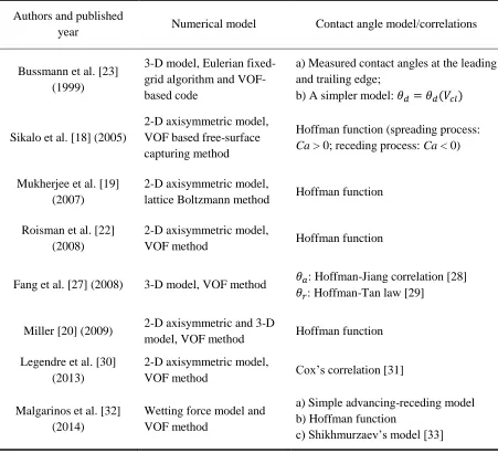
Table 2.1: Correlations Used in DCA Simulations from Available Literature

Authors and published

year Numerical model Contact angle model/correlations

Bussmann et al. [23] (1999)

3-D model, Eulerian fixed-grid algorithm and VOF-based code

a) Measured contact angles at the leading and trailing edge;

b) A simpler model: 𝜃𝑑= 𝜃𝑑(𝑉𝑐𝑙)

Sikalo et al. [18] (2005)

2-D axisymmetric model, VOF based free-surface capturing method

Hoffman function (spreading process: Ca > 0; receding process: Ca < 0)

Mukherjee et al. [19] (2007)

2-D axisymmetric model,

lattice Boltzmann method Hoffman function

Roisman et al. [22] (2008)

VOF method Hoffman function

Fang et al. [27] (2008) 3-D model, VOF method 𝜃𝑎: Hoffman-Jiang correlation [28]

𝜃𝑟: Hoffman-Tan law [29]

Miller [20] (2009) 2-D axisymmetric and 3-D

model, VOF method Hoffman function

Legendre et al. [30] (2013)

VOF method Cox’s correlation [31]

Malgarinos et al. [32] (2014)

Wetting force model and VOF method

a) Simple advancing-receding model b) Hoffman function

c) Shikhmurzaev’s model [33]

In this Chapter, a DCA evolution map is created to clarify the fundamental understanding

of Hoffman function and illustrate the DCA evolving mechanism; based on this evolution

map, the Advancing-Receding DCA (AR-DCA) model is proposed and explained, in

(38)

18

Hoffman's experiments. Using User Defined Function (UDF), the Hoffman function is

implemented into A-DCA and AR-DCA models. Then, with VOF method, a series of

simulations for droplet (water and glycerin) impact on horizontal and inclined surfaces

are conducted based on the A-DCA, AR-DCA and SCA models. The numerical results

from these three models are compared qualitatively and quantitatively to the

corresponding experimental results from Sikalo et al [25, 34].

2.2.Fundamental Understanding of Hoffman Function

From Hoffman’s original experiments [16], it is known that the advancing liquid-air

interface was captured to investigate the relation between the advancing contact angle

and capillary number. Thus, the A-DCA model is developed by following the basic

understanding of Hoffman function, and the Equation (2.2) is utilized to predict the

advancing contact angle. For Ca > 0, 𝐶𝑎 + 𝑓Hoff−1(𝜃𝑠) > 𝑓Hoff−1(𝜃𝑠), then the value of

𝜃_𝑑(𝜃_𝑑 = 𝑓Hoff[𝐶𝑎 + 𝑓Hoff−1(𝜃𝑠)]) will be always greater than that of the static contact

angle 𝜃_𝑠, which refers to the advancing phase. In the previous research work by Miller

[20], the 2-D axisymmetric simulation of water droplet impact on horizontal surface was

conducted with DCA model, which considered only the advancing dynamic contact

angles: the capillary number in the UDF code of Ref. [20] was assumed to be always

positive while the advancing dynamic contact angle was calculated.

In addition to A-DCA model, another method to employ Hoffman function is to consider

both advancing and receding contact angles, defined as AR-DCA model in this thesis.

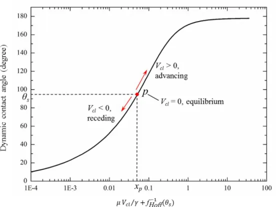
Figure 2.1 shows a dynamic contact angle evolution map which is used to better illustrate

(39)

19

Hoffman’s experiments [16]). We assume a point p on the curve where the liquid system

reaches the equilibrium state and the contact angle at this moment will be the static

contact angle 𝜃𝑠. The x-coordinate of point p, xp, is the shift factor of this liquid system,

because when the contact line velocity Vcl = 0, xp = 𝜇𝑉𝑐𝑙/𝛾 + 𝑓Hoff−1(𝜃𝑠) = 𝑓Hoff−1(𝜃𝑠). When

Vcl > 0, 𝜇𝑉𝑐𝑙/𝛾 + 𝑓Hoff−1(𝜃𝑠) > xp, 𝜃𝑑 = 𝑓Hoff[𝜇𝑉𝑐𝑙/𝛾 + 𝑓Hoff−1(𝜃𝑠)] > 𝜃𝑠, which refers to the

advancing phase (on the right side of point p along the curve as shown in Figure 2.1;

when Vcl < 0, 𝜇𝑉𝑐𝑙/𝛾 + 𝑓Hoff−1(𝜃𝑠) < xp, 𝜃𝑑 = 𝑓Hoff[𝜇𝑉𝑐𝑙/𝛾 + 𝑓Hoff−1(𝜃𝑠)] < 𝜃𝑠, which refers

to the receding phase (on the left side of point p along the curve as shown in Figure 2.1.

Figure 2.1: Dynamic contact angle evolution map.

2.3.Numerical Methodology

In this study, by creating a UDF code in ANSYS Fluent, the A-DCA and AR-DCA

models are developed with the implementation of DCA at the wall boundary. The VOF

(40)

20

2.3.1. Governing Equations with Volume of Fluid (VOF) Method

The mass conservation equation is expressed as:

𝜕(𝜌)

𝜕𝑡 + ∇ ∙ (𝜌𝑢⃑ ) = 0 (2.3)

In the VOF model, the gas and liquid phases can be considered as a two-phase mixture

flow. The mixture density and viscosity can be calculated by:

𝜌 = 𝑠_𝑙𝜌_𝑙+ 𝑠_𝑔𝜌_𝑔 (2.4)

𝜇 = 𝑠𝑙𝜇𝑙+ 𝑠𝑔𝜇𝑔 (2.5)

where 𝑠_𝑙 is the volume fraction of liquid phase and 𝑠_𝑔 is the volume fraction of gas phase.

The sum of the volume fraction is:

𝑠𝑙+ 𝑠𝑔 = 1 (2.6)

The interface between the gas and liquid phase is tracked by solving the continuity

equation for the volume fraction of one of the phases, e.g., for liquid phase:

𝜕(𝑠_𝑙𝜌_𝑙)

𝜕𝑡 + ∇ ∙ (𝑠𝑙𝜌𝑙𝑢⃑ ) = 0 (2.7)

A single momentum equation is given by:

𝜕

𝜕𝑡(𝜌𝑢⃑ ) + ∇ ∙ (𝜌𝑢⃑ 𝑢⃑ ) = −∇𝑝 + ∇ ∙ [𝜇(∇𝑢⃑ + ∇𝑢⃑

T_{)] + 𝑆}

𝑚 (2.8)

(41)

21

be expressed as:

𝑆_𝑚 = 𝜌𝑔 + 𝛾𝜅 𝜌∇𝑠𝑙

(𝜌𝑙+ 𝜌𝑔)/2

(2.9)

where 𝛾 is the surface tension coefficient and 𝜅 is the surface curvature.

For the numerical simulation for droplet impact on horizontal and inclined surface in this

study, the time step is set as 1×10-6_{s for all the cases to keep the Courant number (Co)}

less than 0.5, in order to ensure the calculation stability.

2.3.2. Implementation of Contact Angle Models

Using ANSYS Fluent, the SCA model is employed with the input static contact angle 𝜃_𝑠

at the wall boundaries. The surface unit normal 𝑛̂ is determined by:

𝑛̂ = 𝑛̂_𝑤cos 𝜃_𝑠+ 𝑡̂_𝑤sin 𝜃_𝑠 (2.10)

where 𝑛̂_𝑤 and 𝑡̂_𝑤 refer to the unit vectors normal and tangential to the wall respectively.

In A-DCA and AR-DCA models, Equation (2.11) is used instead of Equation (2.10):

𝑛̂ = 𝑛̂_𝑤cos 𝜃_𝑑+ 𝑡̂_𝑤sin 𝜃_𝑑 (2.11)

𝜃_𝑑 is the dynamic contact angle applied at the wall boundaries through a UDF code based

on the Hoffman function, i.e., Equation (2.1) and (2.2).

In order to implement the DCA models, the authors have used the original UDF code

from Ref. [20] to try a few simple tests and found that it did not work properly for our

(42)

22

capillary number Ca to be the absolute value of 𝜇𝑉𝑐𝑙/𝛾, i.e., 𝐶𝑎 = 𝜇|𝑉𝑐𝑙|/𝛾. Therefore,

for the results reported in this Chapter, we build our own UDF code to implement both

A-DCA and AR-A-DCA models, based on the experience we learned through testing the

original UDF code in Ref. [20].

2.4. Numerical Model Description

2.4.1. Experiments for Validation

Sikalo et al. [25, 34] conducted a series of experiments for droplet impact on horizontal

and inclined surfaces, and investigated the droplet dynamic behaviors and phenomena. A

schematic diagram for the droplet impact on the inclined surface in the experiment is

shown in Figure 2.2: the droplet falls down vertically with an angle α between the falling

direction and the surface. In the case of the horizontal surface, the angle α becomes 90°.

Figure 2.2: Schematic of droplet impact on a surface [25].

In the present study, four cases are selected and simulated: 1) glycerin droplet impact on

horizontal smooth glass [34]. 2) water droplet impact on smooth glass (α = 45°) [34]; 3)

water droplet impact on smooth glass (α = 10°) [25]; 4) water droplet impact on wax (α =

(43)

23

in Table 2.2.

Table 2.2: Detailed Liquid Property, Surface Wettability and Impact Velocity for Selected Cases

Case

# Liquid

Initial droplet diameter

D (mm)

Impact angle α

(°)

Surface tension γ (N/m)

Viscosity µ (mPa·s)

Density ρ (kg/m3)

𝜽𝒂− 𝜽𝒓

(°)

Weber number

(We)

Impact velocity Vp (m/s)

1 Glycerin 2.45 90 0.063 116 1220 17-13 391 2.871

2 Water 2.7 45 0.073 1.0 996 10-6 391 3.253

3 Water 2.7 10 0.073 1.0 996 10-6 391 3.253

4 Water 2.7 10 0.073 1.0 996 105-95 391 3.253

2.4.2. Computational Domain and Input Parameters

For the numerical simulation, a three-dimensional cylinder computational domain is

employed in the present study, as shown in Figure 2.3(a), with the radius (R) of 7.5 mm

and height (H) of 4 mm. The direction of gravity is set along the negative Y-axis. The

mesh type is triangular wedge and a refinement of the mesh near the bottom wall is

conducted in order to better simulate the droplet interface near the boundary wall. The

no-slip boundary condition is applied on the bottom wall. The pressure-inlet boundary is

implemented on the remaining surfaces to represent the surrounding atmosphere with

gauge total pressure set as zero. Figure 2.3(b) is a schematic of the droplet initial and

impact positions in the computational domain. In the beginning of the numerical

simulation, the droplet is patched in the domain with an initial velocity V0 (negative

Y-axis direction) and falling distance d0in order to achieve the impact velocity Vp in the

corresponding experiment. The input SCA in the simulation for the shift factor 𝑓_Hoff−1 (𝜃_𝑠)

is determined by the equilibrium value between θa and θr. The detailed input parameters

(44)

24

First, in order to ensure the computational domain is sufficiently reliable for the

simulation, the effect of domain size on the simulation results is tested based on the

current domain (R = 7.5 mm and H = 4 mm) and another domain with larger radius (R =

9 mm and H = 4 mm). Figure 2.4(a) and (b) show the comparison of the ratio l/h (droplet

spreading length/droplet apex height) in terms of a dimensionless time t* (t* = t·Vp/D

[25], where t is the time from impact) based on these two domains for Case 1 and Case 2

respectively and the results are nearly identical, indicating that the increase of domain

size has no significant effects on the simulation for droplet deformation.

(a) (b)

Figure 2.3: (a) Schematic of computational domain used in the numerical simulation; (b) Schematic of the droplet initial and impact position in the computational domain (side-view).

Table 2.3: Simulation Parameters for Selected Cases

Case # Droplet initial velocity V0 (m/s)

Falling distance d0

(mm)

Impact time ti (ms)

Droplet Impact velocity Vp

(m/s)

Input SCA (°)

1 2.867 1.225 0.42 2.871 15

2 3.250 1.100 0.33 3.253 8

3 3.250 1.100 0.33 3.253 8

(45)

25

(a) (b)

Figure 2.4: Effects of computational domain size on the numerical results: (a) Case 1; (b) Case 2.

2.4.3. Mesh Independency

In the present study, the mesh independency is performed by applying different number

of nodes along the side edge (i.e., the direction along the height (H = 4 mm)) and the

bottom edge. The information of different grid resolutions is shown in Table 2.4.

Table 2.4: Information of Different Grid Resolutions in the Present Study

Grid Resolution

Type

Number of nodes along the height

(H)

Number of nodes along the

bottom edge

Total number of nodes (approximately)

Maximum cell volume

(mm3)

Minimum cell volume

(mm3)

A 21 235 108,000 6.09×10-3 1.34×10-3

B 41 471 835,000 9.24×10-4 1.43×10-4

C 68 589 2,160,000 4.83×10-4 3.69×10-5

D 81 673 3,345,000 3.16×10-4 1.98×10-5

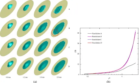
Figure 2.5 and Figure 2.6 show the numerical results under different grid resolutions

(under Case 1 and 2) for both qualitative and quantitative comparisons. It can be noted

that for the glycerin droplet impact on horizontal surface (Case 1), the droplet profile

(46)

26

B, C and D is quite similar, as shown in Figure 2.5(a). However, from Figure 2.5(b), it

can be seen that the evolutions of l/h versus t* from all the grid resolution types are close

before approximately t* = 1.6; after that, the values of l/h from Resolution C and D (finer

grid) have a sudden drop at about t* = 2.0, which is not reflected in coarser grids

(Resolution A and B). For the water droplet impact on 45° inclined surface (Case 2), an

obvious improvement on the simulation quality can be observed from Resolution A and

B to Resolution C and D, as shown in Figure 2.6(a): under coarse grid (Resolution A), the

droplet forms liquid slug when it slides along the surface while under Resolution B, C

and D, the droplet can fully spread on the surface and form liquid film; also, for the last

profile (2.0 ms), the leading edge of the liquid film breaks up into small parts under

Resolution B whereas the finer grid (Resolution C and D) can generate smooth rim and

the major features are identical. The quantitative comparison for Case 2 (Figure 2.6(b))

also shows that the Resolution A results in lower value of l/h. Considering the increased

computational cost with the increase of the number of nodes, the grid resolution type C is

adopted for all the four cases in the present study.

(a) (b)