A General Method for Calculating Likelihoods Under the Coalescent Process

(1)

INVESTIGATION

A General Method for Calculating Likelihoods Under

the Coalescent Process

K. Lohse,* R. J. Harrison,†_{and N. H. Barton*},‡,1 *Institute of Evolutionary Biology, University of Edinburgh, Edinburgh EH9 3JT, United Kingdom,†East Malling Research, East Malling ME19 6BJ, United Kingdom, and‡Institute of Science and Technology, A-3400 Klosterneuburg, Austria

ABSTRACTAnalysis of genomic data requires an efficient way to calculate likelihoods across very large numbers of loci. We describe a general method for finding the distribution of genealogies: we allow migration between demes, splitting of demes [as in the isolation-with-migration (IM) model], and recombination between linked loci. These processes are described by a set of linear recursions for the generating function of branch lengths. Under the infinite-sites model, the probability of any configuration of mutations can be found by differentiating this generating function. Such calculations are feasible for small numbers of sampled genomes: as an example, we show how the generating function can be derived explicitly for three genes under the two-deme IM model. This derivation is done automatically, usingMathematica. Given data from a large number of unlinked and nonrecombining blocks of sequence, these results can be used to find maximum-likelihood estimates of model parameters by tabulating the proba-bilities of all relevant mutational configurations and then multiplying across loci. The feasibility of the method is demonstrated by applying it to simulated data and to a data set previously analyzed by Wang and Hey (2010) consisting of 26,141 loci sampled from Drosophila simulansandD. melanogaster. Our results suggest that such likelihood calculations are scalable to genomic data as long as the numbers of sampled individuals and mutations per sequence block are small.

T

HE coalescent process is highly variable: samples from even a single well-mixed population rapidly coalesce down to a few ancestral lineages, so that their deeper an-cestry is determined by just a few random coalescence events (Felsenstein 1992). Thus, small samples taken from a large number of loci give much more information than large samples from a few loci. For example, the distribution of coalescence times, and hence the history of effective population size, has been inferred from single diploid ge-nomes (Li and Durbin 2011). Although it is now feasible to sample very large numbers of markers, or indeed whole genomes, we urgently need methods for analyzing such data. In principle, we can calculate likelihoods from very large data sets, if we have loosely linked blocks of sequence within which recombination is negligible. Provided that only a few genomes are sampled, we can tabulate the prob-ability that any particular conﬁguration of mutations will

be seen at each locus and then multiply across large num-bers of loci to ﬁnd the likelihood of our model (Takahata

et al.1995).

Wilkinson-Herbots (2008) and Wang and Hey (2010) derive the distribution of coalescence times for a pair of genes sampled from two populations that separated at some time in the past and subsequently exchanged migrants. This “isolation-with-migration”(IM) model is of particular inter-est in evaluating the role of gene ﬂow during speciation. Hobolthet al.(2011) show how this and similar calculations can be done more efﬁciently using matrix exponentials.

Here, we present an alternative method, based on gener-ating functions, which provides direct information about the pattern of mutational variation and can be automated using symbolic algebra packages such asMathematica. We give the IM model as an example and show how the method extends to linked loci.

The Generating Function of a Genealogy

The ancestry of a sample of genes, V, is described by the lengths of the branches that are ancestral to every possible subset. For example, suppose that we have three genes at a locus, labeledV¼{a,b,c}. We label lineages by the set Copyright © 2011 by the Genetics Society of America

doi: 10.1534/genetics.111.129569

Manuscript received April 13, 2011; accepted for publication August 18, 2011 Supporting information is available online at http://www.genetics.org/content/ suppl/2011/09/07/genetics.111.129569.DC1.

1_{Corresponding author: Institute of Science and Technology, Am Campus 1, A-3400} Klosterneuburg, Austria. E-mail: [email protected]

(2)

of genes to which they are ancestral. Thus, if lineages an-cestral to genes band c coalesced most recently, then the branches {b} and {c} have the same length;i.e.,t{b}¼t{c}, and t{a} ¼ t{b} 1 t{b,c}. With this topology, there are no lineages ancestral to {a,b} or {a,c} andt{a,b}¼ t{a,c}¼ 0. Thus, both the topology and the branch lengths are encoded by the vector of all possible branchest, which has elementstS forS4V.

The generating function (GF) for the branch lengths t

depends on a set of corresponding dummy variables, v and is defined as the expectationc½v ¼E½e2v:t_{. It is more} convenient to use this form—a Laplace transform—rather than the alternative E½QS4VztSS. Generating functions are widely used, primarily because the distribution of the sum of two independent variables is given by the product of the corresponding GF. In particular, Latter (1973) used a GF approach to find the solution for the expected frequency of heterozygotes under the symmetric IM model and Griffiths (1981b) used the GF for the numbers of types to calculate sampling distributions for the infinite-alleles model. Griffiths (1991) applied this to the two-locus prob-lem (see also Jenkins 2008). In the context of the coales-cent, the GF has a concrete interpretation: under the infinite-sites model, it is the probability of seeing no muta-tions, given mutation ratevSalong branchS.

Information about the branch lengths themselves can be recovered from the GF. The mean lengths, E[tS], are found by differentiating with respect to vS and setting v to zero; higher moments are found by differentiating more than once. The actual distribution can be found by taking the inverse Laplace transform, which may be done either algebraically (if the GF has a certain form) or by numerical integration.

In practical applications, we wish to know the probability that there arekSmutations on branchS. Under the inﬁ nite-sites model, with mutation ratem, this is given by taking the expectation of a Poisson distribution with meanmtover the distribution of coalescence times,

P½kS ¼E "

e2mtSðmtSÞ

kS

kS!

#

¼ð2mÞ kS

kS!

@kSc

@vkS

S

!

vS¼m

; (1)

which is proportional to thek9Sth differential of the GF with respect tovS, taken atvS¼m, and setting all otherv’s to zero. We see that Equation 1 defines a term in a Taylor series, so that the probability of a particular configuration of mutations is given by the coefficient in the expansion ofc. In other words, if we setvS¼m2xSand expand around the pointxS¼0, then the probability of seeingkSmutations on branchSis the coefficient ofxkS

S , multiplied bym

kS_{. Similarly,}

the joint probability of seeing a conﬁguration ofkS1;kS2;. . .

mutations on branches S1, S2, . . . is the coefﬁcient of xkS₁

S1 x

kS₂

S2 . . ., multiplied by m

kS1þkS2.... In the following, we

scale time relative to twice the effective population size, 2N;i.e., the scaled mutation rate is 2Nm¼u/2.

While we assume an inﬁnite-sites mutation model for simplicity throughout, the GF can also be used to obtain the probabilities of mutational conﬁgurations for more complex mutation models. For example, under the Jukes-Cantor (Jukes and Jukes-Cantor 1969) model mutations to a dif-ferent state happen at rate (3/4)mand the chance of a back mutation is (1/4)m. The probabilities that two sequences differ or are the same at any particular site are 3ð12e2mt_Þ₌₄ and ð1þ3e2mt_Þ₌₄_; _{respectively. Given a pair of sequences} of length n the probability of seeing j sites in a different andn2jin the same state is given by taking the expectation of a Binomial distribution over the distribution of coalescence times:

P½j ¼E

3 4

n

12e2mtj

1 3þe

2mt

n2j n

j

: (2)

This can be written as a sum of the GFs of pairwise coalescence times:

P½j ¼

3 4

n_Xj

k¼0

X n2jþk

a¼k

ð21Þk

1 3

n2j2aþk n j j k n2j a2k

c½ma:

(3)

Thus, in principle, we can obtain results under aﬁnite-sites mutation model directly from the GF without the need to take derivatives.

The generating function is a sum of terms, each corre-sponding to a particular topology. For a given topology, many branches will have zero length by definition, and so the GF will be independent of the corresponding vS; some branches will have the same lengths (e.g.,t{b}¼t{c}) and so the corresponding terms will be a function of the sum of the respective dummy variables (e.g.,v{b} 1 v{c}). Under the infinite-sites model, this brings a substantial simplification if we see mutations on internal branches, because any terms that do not depend on the corresponding dummy variables can be dropped from the GF: they represent topologies in-consistent with the data. The joint likelihood for a given mutational configuration can then be calculated by multiple differentiation of the remaining terms, which involves a sum over only the possible topologies.

The General Recursion

The recursion for the generating function of genealogical branch lengths can be derived by tracing back from the present to the most recent event, which might be a co-alescence, a recombination, a movement between demes, a change in population structure, or whatever. Eventsioccur at rate liand (tracing back in time) change the confi gura-tion of genes from the sampling configurationVtoVi. Con-figurations include the number of lineages and—depending on the model—their locations and/or genetic backgrounds. For example, suppose that we start with three lineages {a},

(3)

{b}, and {c}. A coalescence between lineages {b} and {c} generates a new conﬁguration {{b,c}, {a}}, in which there are now two lineages—one ancestral to {b,c} and the other to {a}. We derive a recursion that expresses the GFc[V] as a sum over the possible conﬁgurations before the previous event. The time back to that event is exponentially distrib-uted with ratePili, and so the distribution of the lengths of the terminal branches is just the convolution of this with their previous distribution. Taking Laplace transforms, this corresponds simply to multiplication by the factor 1=ðPiliþ

P

jSj¼1vSÞ, since a convolution of distributions transforms to a product of the previous GF and the GF of an exponential distribution with rate Pili. Summing over all possible events we have

c½V ¼

P

ilic½Vi

P

iliþ

P

jSj¼1vS

: (4)

The denominator gives the total rate of events, Pili in the interval from the present to the first event, plus the sum of the vS that correspond to terminal branches (the “leaves”of the tree). The numerator is the sum over all possible generating functions at the previous event; Videnotes the configuration prior to eventi. This recursion yields a set of linear equations for thec[V] that is readily solved; the limit is set by the number of possible sample configurations of genes that have to be tracked. To see how this works, we give a series of examples.

A Single Population

In the simplest case of a single well-mixed population, we need to track only coalescence events. Scaling time relative to twice the effective population size, 2N, the rate of coales-cence is given by the number of pairs of lineages in a given sample conﬁgurationjV₂j¼jVjðjVj21Þ=2;where there are |V| lineages. Thus

c½V ¼ 1

jVj

2

þP_jSj¼1vS

X

fx;yg4V

cV_fx_;_yg; (5)

where the sum is over all thejV₂jpossible pairwise coales-cences, between genes x and y. Vfx;yg denotes the sample conﬁguration after coalescence,i.e.,Vwith lineages {x}, {y} replaced by the new lineage {x,y}. Since we deﬁne the GF for a single gene as 1, we have for two genes

c½a;b ¼_ð 1

1þvaþvbÞ:

(6)

This is equivalent to the probability of identity in state with

va+vb¼u. Note that for brevity, we have condensed the notation so thatc[a,b] represents the GF for two lineages ancestral to genesaandb, respectively; andc[ab,c] repre-sents two lineages, one ancestral toaandb, and the other

to c. For automated recursions (File S1), the full (and un-ambiguous) notation c[v, {{a}, {b}}], c[v, {{a,b}, {c}}] would be used. For three genes

c½a;b;c ¼ 1

ð3þvaþvbþvcÞ ·

1

ð1þvabþvcÞ

þ 1

ð1þvacþvbÞ

þ 1

ð1þvbcþvaÞ

:

(7)

Each of the three terms corresponds to one of the three possible topologies. For example, the last term depends on

vbcand corresponds to coalescence between {b} and {c}, so that the interior branch tbc .0. To ﬁnd the probability of each topology, we set all the vSto zero, and see that each term contributes 1

3. Toﬁnd the probability that there arek mutations ancestral tobandc, we differentiatektimes with respect tovbc, setvbcto equal the scaled mutation rateu/2 and all other vS to zero, and multiply by (2u/2)k/k! (Equation 1). This gives the geometric distribution

ð1=3Þð2uk₌_ð₂_þ_uÞkþ1_Þ

fork.0, the factor 3 arising because there is a 1/3 probability thatbandccoalesceﬁrst, allowing mutations of this class to exist. Alternatively, we could set all the vS to 0, except for vbc¼u=22xbc, and then expand around xbc ¼0; the coefﬁcients ofxkbcbc are proportional to the chance of seeing kbc mutations that are ancestral to

b and toc. The joint probabilities of other mutational con-ﬁgurations can be found in a similar way.

Migration

Suppose that two populations exchange migrants at a scaled rate 2Nm. For simplicity, we assume that migration is symmetric and both demes are of the same size (the gener-alization to more demes, different population sizes, and asymmetric migration is obvious) and that a setV1of genes is sampled from one deme and V2 from the other. Now, there can be coalescence, which reduces the size of one or the other set, or migration, which transfers a lineagexfrom one deme to the other creating, for example, new sample conﬁgurationsV1,+xandV2,2x. Thus

c½V1;V2

¼_j_V 1

1j 2 þ _j_V 2j 2

þ2NmðjV1j þ jV2jÞ þPS4V1;jSj¼1vSþ

P

S4V2;jSj¼1vS

· P

fx;yg4V1

cV1;fx;yg;V2þ P

fx;yg4V2

cV1;V2;fx;yg

þ 2Nm P fxg4V1

cV1;2x;V2;þxþ2Nm P

fxg4V2

cV1;þx;V2;2x

! :

(8)

This leads to a set of linear equations that can readily be solved. We need to distinguish only sample conﬁgurations where the genes are in different demes, c[a\b], or in the same demes,c[a,b\Ø], say (again, we have condensed the notation; Ø represents the empty set, and \ the separation between the two demes). From Equation 8 and using the symmetry of the model,

(4)

c½anb ¼_ð 2Nm

4NmþvaþvbÞ

ðc½a;bnø þc½øna;bÞ

¼ 4Nm

ð4NmþvaþvbÞ

c½a;bnø

c½a;bnø ¼ 1

ð1þ4NmþvaþvbÞ

· ðc½abnø þ2Nmðc½anb þc½bnaÞÞ

¼_ð 1

1þ4NmþvaþvbÞ

ð1þ4Nmc½anbÞ:

(9)

This has the solution

c½anb ¼ M

ðMþvaþvbÞð1þMþvaþvbÞ2M2

c½a;bnø ¼ Mþvaþvb

ðMþvaþvbÞð1þMþvaþvbÞ2M2;

(10)

whereM¼4Nm. Note that the GF is a function only ofva1

vb, given the constraintta¼tb. Equation 10 has been pre-viously derived as the probability of identity in state with

va1vb ¼u(Grifﬁths 1981a, equation 10). Taking the in-verse Laplace transform gives the probability of pairwise coalescent times,

Pa;bnø½t ¼

1 2

e2l0t

12 1

l12l0

þe2l1t

1þ 1

l12l0

P_anb½t ¼M

e2l0t2e2l1t

l12l0 ;

(11)

where l0¼1₂ð1þ2M2

ffiffiffiffiffiffiffiffiffiffiffiffiffiffiffiffiffiffi 1þ4M2 p

Þ and l1¼1₂ð1þ2Mþ ffiffiffiffiffiffiffiffiffiffiffiffiffiffiffiffiffiffi

1þ4M2

p

Þ. This result was derived directly by Herbots (1997), using a partial fraction expansion (see Grifﬁths 1981a; Wilkinson-Herbots 2008, equation 18), but can also be found from the discrete time transition matrix (Wakeley 1996). In fact,l0andl1are the eigenvalues of the symmet-ric transition matrixQgiven by Hobolth et al.(2011) with

S1¼S2,S11¼S22, andm1¼m2.

Population Splits: The IM Model

Now, suppose that the two populations derive from a single ancestral population T generations ago. Dealing with finite times explicitly leads to complicated expressions (Wang and Hey 2010). However, we can retain the simple form of the GF by taking the Laplace transform with respect to the divergence time, with dummy variableL. This has a concrete interpreta-tion, as the expectation over a model in which the divergence time is exponentially distributed with rateL, times a normal-izing factorL. We can eitherfit this model directly or take the inverse Laplace transform with respect toL, tofind the GF of the genealogy for a given divergence timeT, which we denote

P. (More precisely, we take the inverse Laplace transform of

L21_c_{, since}_c_¼_E_½_e2LT_P_¼RN 0Le2

LT_PdT_.)

The recursion is now

c½V1;V2

¼ 1

Lþ

jV1j

2

þ

jV2j

2

þ2NmðjV1j þ jV2jÞ þPS4V1;jSj¼1vSþ

P

S4V2;jSj¼1vS

· Lc½V1[V2 þ P

fx;yg4V1

cV1;fx;yg;V2

þ P

fx;yg4V2

cV1;V2;fx;yg

þ 2Nm P fxg4V1

cV1;2x;V2;þx

þ2Nm P fxg4V2

cV1;þx;V2;2x

! :

(12)

The additional termLc[V[V] represents the replacement of the GF for two separate demes by the GF for a single popula-tion, which follows the standard coalescent (see Equation 5). Expression (12) is otherwise identical to Equation 8.

As a simple example, consider two genes,

c½anb ¼_L 1 þ4Nmþvaþvb

· ðLc½a;b þ2Nmðc½øna;b þc½a;bnøÞÞ

¼_L_þ 1

4Nmþvaþvb·

_L

ð1þvaþvbÞþ

4Nmc½a;bnø

c½a;bnø ¼_L 1

þ1þ4Nmþvaþvb

· ðLc½a;b þc½abnø þ2Nmðc½anb þc½bnaÞÞ

¼_L 1

þ1þ4Nmþvaþvb

_L

ð1þvaþvbÞþ

1þ4Nmc½anb

;

(13)

which have a solution similar to Equation 10:

c½anb ¼ 1

1þvaþvb

· Lð1þLþvaþvbÞ þMð1þ2LþvaþvbÞ

Lþvaþvbþ ðLþvaþvbÞ2þMð1þ2Lþ2vaþ2vbÞ

c½øna;b ¼ 1 1þvaþvb

· Lþvaþvbþ ðLþvaþvbÞ2þMð1þ2LþvaþvbÞ

Lþvaþvbþ ðLþvaþvbÞ2þMð1þ2Lþ2vaþ2vbÞ

:

(14)

With complete isolation (i.e.,M¼0), differentiation of these expressions yields the explicit formula for the numbers of pairwise differences in the complete isolation model given by Takahataet al.(1995).

For three genes we have

c½anb;c ¼_L 1

þ1þ6Nmþvaþvbþvc

· ðLc½a;b;c þc½anbc þ2Nmðc½øna;b;c þ c½cna;b þc½bna;cÞÞ

c½øna;b;c ¼_L_þ 1

3þ6Nmþvaþvbþvc

· ðLc½a;b;c þc½øna;bc þc½ønab;c þc½ønac;b þ 2Nmðc½anb;c þc½bna;c þc½cna;bÞÞ:

(15)

Although there are only two types of conﬁguration with three genes, there are three permutations of theﬁrst. Thus,

(5)

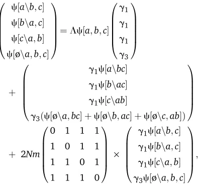
in our symmetric model, we have four coupled linear equations, which can be written in matrix form,

0 B B B B @

c½anb;c c½bna;c c½cna;b c½øna;b;c

1 C C C C

A¼Lc½a;b;c 0 B B B B @ g₁ g₁ g₁ g₃ 1 C C C C A þ 0 B B B B @

g₁c½anbc g₁c½bnac g₁c½cnab

g₃ðc½øna;bc þc½ønb;ac þc½ønc;abÞ 1 C C C C A

þ 2Nm 0 B B B B @

0 1 1 1

1 0 1 1

1 1 0 1

1 1 1 0

1 C C C C A ·

0 B B B B @

g₁c½anb;c g₁c½bna;c g₁c½cna;b g₃c½øna;b;c

1 C C C C A;

where gj¼1=ðLþjþ6NmþvaþvbþvcÞ and j is the number of pairs that can coalesce given a particular sample conﬁguration.

This has an explicit solution, which we derive in detail in File S1using a simple symbolic algorithm. If the demes were not equivalent because of asymmetric migration and/or dif-ferences in effective population size, then we would need to distinguish conﬁgurations such as c[a\b, c] and c[b, c\a] and would have eight coupled equations.

With coalescence or population splits alone, the recur-sions can be solved directly: every event leads back to a simpler configuration, with either fewer lineages or fewer demes. However, with migration, we must solve a set of coupled equations. This is easily done numerically, for specific v, but beyond the simplest cases leads to cumbersome algebraic expressions that cannot readily be differentiated. One way around this problem (which we employ inFile S1) is to condition on the topology. Another simplification is to expand the GF in M ¼4Nm, writing

c¼PNi¼0Mici. Then, each migration event leads back to a lower-order expression, and we can againﬁnd the solu-tion directly. This procedure is equivalent to separating out the GF into a sum of terms, each corresponding to 0, 1, 2,. . .migration events.

In comparison, it is straightforward to obtain results for summaries of the genealogy from the GF. For instance, the distribution of the total number of mutationsXcan be found by setting allvto be the same and taking the inverse Lap-lace transform (see File S1). Similarly, the probability of a particular topology can be found by taking the limit of thevScorresponding to internal branches that are incompat-ible with this topology at inﬁnity with all othervSevaluated at zero. For a triplet with sampling conﬁguration {a\b,c} this gives

P½fa;fb;cgg ¼ lim vab/N vac/N

c½anb;cjvS¼0¼

2Mþ322e2ð1þ2MÞT 3ð1þ2MÞ

P½fc;fa;bgg ¼P½fb;fa;cgg ¼ lim vab/N vbc/N

c½anb;cjvS¼0¼

2Mþe2ð1þ2MÞT 3ð1þ2MÞ :

(16)

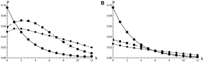
For the case of three genes in the IM model Equation 16 yields Figure 1. Furthermore, for a given topology, {a, {b,c}} say, one can ﬁnd the distribution of the number of muta-tions on the internal branch,P[kbc|{a, {b,c}}], by differen-tiating the limit in Equation 16 with respect to vbc and setting all othervSto zero as before. Plotting these distri-butions (Figure 2) reveals that genealogies congruent with the sampling, i.e., with topology {a, {b, c}}, tend to have a longer internal branch than those with incongruent topol-ogies {b, {a,c}} or {c, {a,b}} (Figure 2Avs.2B). This is to be expected, given that coalescence events between lineages sampled from the same population, in this case {b,c}, occur relatively faster, leaving a long timetbcduring which muta-tions can occur on the internal branch. In contrast, coales-cence events between lineages sampled from different populations are likely to occur deeper in the past, within the ancestral population. These new results extend previous theory on pairwise coalescence times in the IM model (Wilkinson-Herbots 2008; Wang and Hey 2010) to topolog-ically informative samples. Likewise, it is straightforward to use the GF to extend pairwise results for the IM model beyond the two-deme case. Larger numbers of populations (d) would be incorporated into Equation 9 by an additional term (d 2 1); e.g., the rate at which pairs of lineages in different demes are brought together in the same population becomesM/(d21).

Figure 1 Topological probabilities (Equation 16) for a sample of three genes in the IM model, plotted against the scaled migration rateMfor two splitting times,T¼0.5 (solid lines) andT¼2 (dashed lines). The chance of observing an incongruent genealogy with topology {c, {a,b}} or {b, {a,c}} (bottom) increases withM, as congruent topologies {a, {b,c}} (top) become less likely.

(6)

Recombination Between Linked Loci

The GF method readily extends to multiple linked loci. Each individual is represented as a list, which for each locus gives the set of genes to which it is ancestral; Figure 3 gives an example with three loci. Suppose that we havekindividuals, carrying lineagesV¼V1,. . .,Vk,

c½V ¼ 1

k 2

þ2NPa2RraþvL

P

1#i,j#k

c½V_i_;_j_þ₂_N P

a2Rrac½Va !

;

(17)

where vL¼ Pk

i¼1 P

S4Vi;jSj¼1vS, i.e., we need to sum the

vSleaves over both loci and individuals,Ris the set of all possible recombination events and rais the rate of a re-combination of type a2R. The ﬁrst sum on the right in Eq. (4) is over allk2

possible coalescences between thek

individuals. At each coalescence, the lists of genes at each locus are merged. For example, a coalescence between {a, p, x} and {ø,q, ø} gives an ancestral lineage {a,pq,

x}, in which the second locus is now ancestral to genes p

and q. The second sum on the right is over all possible recombination events a2R, each resulting in a new set of lineages Va; these increase the number of lineages to k 11. For example, a recombination in the parent of an individual {b,q,y}, between theﬁrst locus and the other two, gives two ancestral lineages {b, ø, ø} and {ø, q,y} (Figure 3). Note that this recursion does capture the non-Markovian nature of recombination: the distribution of coa-lescence times at a locus depends on the genealogies at all the other loci, not just the adjacent locus. The GF gives the joint distribution of genealogies rather than the full ancestral re-combination graph (which includes additional information about which loci were carried by the ancestors).

Consider the simplest case, of two genes at two loci; when these are in two individuals, the conﬁguration is denoted {a,x}, {b,y} andvL¼va1vb1vx1vy:

c½fa;xg;fb;yg ¼₁_þ₄_Nr1_þ_v

Lð

c½fab;xyg þ2Nrc½fa;øg;fø;xg;fb;yg þ c½fa;xg;fb;øg;fø;ygÞ

c½fa;øg;fø;xg;fb;yg ¼ 1 3þ2NrþvLð

c½fa;xg;fb;yg þc½fa;øg;fb;xyg þ c½fab;yg;fø;xg þ 2Nrc½fa;øg;fø;yg;fb;øg;fø;ygÞ c½fa;øg;fø;xg;fb;øg;fø;yg ¼₆_þ1_v

Lð

c½fa;xg;fb;øg;fø;yg þc ½fa;øg;fø;xg;fb;yg þ c½fab;øg;fø;xg;fø;yg þ c½fø;xyg;fa;øg;fb;øg þ c½fa;yg;fø;xg;fb;øg þc½fb;xg;fa;øg;fø;ygÞ:

(18)

By symmetry, we need only these three recursions, for the cases where the four genes are distributed over two, three, or four individuals. Note that c[{ab,xy}]¼ 1,c[{a, ø}, {b, xy}]¼ c[{a}, {b}], and so on, connecting these two-locus recursions to the one-two-locus GF.

This has the solution

c½fa;xg;fb;yg

¼ 2

9þRþ6RfþR2fþ ð9þRþ2RfÞvLþv2L

18þ26Rþ4R2_þ₂₇_þ₁₉_R_þ₂_R2_v

Lþ ð10þ3RÞv2Lþv3L

c½fa;øg;fø;xg;fb;yg ¼ 6þ

6þ13Rþ2R2fþ ð1þ ð7þ3RÞfÞvLþfv2L

18þ26Rþ4R2_þ₂₇_þ₁₉_R_þ₂_R2_v_L_{þ ð}₁₀_þ₃_R_Þ_v2

Lþv3L

c½fa;øg;fø;xg;fb;øg;fø;yg

¼ 4þ

7þ13Rþ2R2_f_{þ ð}₈_þ₃_R_Þ_fv

Lþfv2L

18þ26Rþ4R2_þ₂₇_þ₁₉_R_þ₂_R2_v

Lþ ð10þ3RÞv2Lþv3L ;

(19)

where f¼1=ð1þvaþvbÞ þ1=ð1þvxþvyÞ, and R ¼ 2Nr. These formulas correspond to those previously obtained by Simonsen and Churchill (1997), using a Markov chain method. For example, the covariance of coalescence times between two loci is

CovTab;Txy

¼ETxyTab

2E½TabE

Txy

; (20)

which can be found straightforwardly from the GF by taking derivatives with respect tovaandvxand evaluating atv¼ 0, noting thatE[Tab]¼E[Txy]¼1:

Figure 2 The distribution of the number of mutations (k) on the internal branches for a sample of three genes {a, {b,c}} in the IM model with symmetric migrationu¼5,M¼0.8 plotted for three different splitting timesT¼0 (circles, solid line),T¼2 (squares, long-dashed line), and T ¼ 4 (diamonds, short-dashed line). Congruent genealogies with topology {a, {b, c}} (A) tend have longer internal branches than those with incongruent topologies {c, {a,b}} or {b, {a,c}} (B). Note that forT¼0 the distributions for the two topologies are identical as expected in a panmictic population.

(7)

CovTab;Txy ¼ d

2_c_½f_a_;_x_g_;_f_b_;_y_g

dvadvx

_v_¼₀

!

21¼ 9þR

9þ13Rþ2R2:

(21)

This agrees with Simonsen and Churchill (1997, equation 52).

Including recombination leads to sets of coupled linear equations, whose solution involves an unwelcome matrix inversion. As with migration, this problem can be avoided by expanding in powers ofR, which is equivalent to summing over histories that involve 0, 1, . . . recombination events. Moreover, these recombination events are uniformly distrib-uted across the genetic map, and so we have a description of the ancestry of the whole genome and not just of two linked loci. The recursions give us the probability that there are no recombination events, that there is one event producing two blocks with different genealogies, that there are three events producing three blocks of genome, and so on. This may allow likelihoods to be calculated for short sequence blocks, provided that Ris small.

Slatkin and Pollack (2006) calculate the probabilities of alternative topologies for genes at two loci in three com-pletely isolated species; their recursion is essentially the same as ours, but tracks just the distribution of topologies rather than the full distribution of coalescence times. Since no coalescence can occur until two of the genes are brought together in the same ancestral population prior to the most recent speciation event, this reduces to the case of three linked pairs of genes in two completely isolated species. This

case can be solved by the above method, by including a rate of population splits, L, which corresponds to the time, T, between the two speciation events.

Drosophila melanogaster–D. simulansDivergence

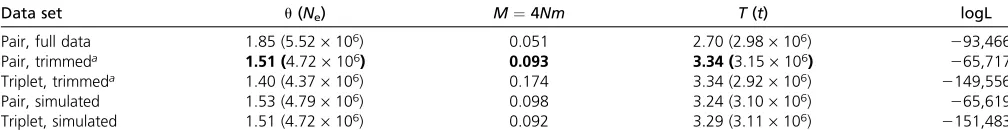
To illustrate the feasibility of the GF method for inference in practice, we applied it to both real and simulated data. We first reanalyzed the genomic data set of Drosophila mela-nogaster–D. simulans compiled and analyzed by Wang and Hey (2010), using a likelihood method for pairwise samples. The data (kindly provided by Y. Wang) consist of alignments of 30,247 blocks of intergenic sequence of 500 bp each sam-pled from two inbred lines of D. simulansand one inbred line each ofD. melanogasterandD. yakuba(the latter used as an outgroup to account for mutational heterogeneity and, in the triplet analysis, to polarize mutations). Following Wang and Hey (2010), low-quality sequences, indels, and positions next to indels were removed. Rather than using the divergence to the outgroup to scale the mutation rate at each locus (Yang 2002; Wang and Hey 2010), each locus was trimmed after afixed number of mutational differences betweenD. yakubaandD. melanogaster. We chose a cutoff of 16 divergent sites, which corresponds roughly to a third of the observed mean divergence across all loci in the full data set. A total of 2,090 loci that were below this cutoff were excluded from the analysis. Since our method assumes infinite-sites mutations, sites with more than two segregat-ing states (12.9% of all polymorphic sites) were excluded. We also filtered out shared derived mutations that were topologically incongruent with the majority class of shared derived mutations in each block (2.5% of all polymorphic sites). A total of 2,016 loci, which contained equal numbers of topologically conflicting shared derived mutations, were excluded. The final, trimmed data set consisted of 26,141 loci. To convert scaled parameter estimates into absolute values (Ne¼ u/4m,t¼g2NeT), we followed Wang and Hey (2010) and assumed thatD. yakubaandD. melanogastersplit 10 MYA and with a generation time per year ofg¼0.1, which gives a mutation rate per block of 8·1028_.

Given that Wang and Hey (2010) detected a signal of gene flow fromD. simulans to D. melanogaster but not in the reverse direction, wefitted an IM model with asymmet-ric migration. The GF for this case can be obtained using Equation 4 and, given that each genealogy can be affected by only one migration event at most, is considerably simpler than the analogous expression with symmetric migration given by solving Equation 15 (details are provided in File S1). To investigate the effect (in terms of bias and power) of including a third sample and thus topology information on parameter estimation, we performed analogous likelihood analyses on pairwise (one sample from each of D. mela-nogaster and D. simulans) and triplet data. To assess the effect of removing positions that violate the infinite-sites mutation model, we also ran a pairwise analysis on the full, untrimmed data set. Mutational heterogeneity in this

Figure 3 An example of coalescence and recombination between three loci. At the present generation (bottom), there are two individuals: one carries genesa,p,xand the other carriesb,q,y. Lineages ancestral to the three loci are colored black, red, and blue, respectively. This is denoted as {{a,p,x}, {b,q,y}}. Tracing back, the most recent event is a recombination (red dot) giving three individuals {{a,p,x}, {b, ø, ø}, {ø,q,y}}, where ø is the empty set. There is then another recombination event, preceded by three coalescence events (black dots); these produce the conﬁgurations {{a,p,x}, {b, ø, ø}, {ø,q, ø}, {ø, ø,y}}; {{a,pq,x}, {b, ø, ø}, {ø, ø,y}}; {{a,pq,x}, {b, ø,y}}; and {{ab,pq,xy}}. Recombination and coalescence events prior to this single common ancestor do not affect the observed genealogy.

(8)

analysis was incorporated by binning loci according to their outgroup divergence and specifying mutation rate scalars for each bin (we used 10 bins).

To speed up calculations in the triplet analysis the GF was conditioned on the topology (by taking limits as shown in Equation 16). Probabilities of all observed mutational conﬁgurations were tabulated separately for each topology class (congruent, incongruent, and topologically uninforma-tive loci) (seeFile S1). Using the FindMaximum function in

Mathematica, the joint likelihood of M, T, and u can be maximized very efﬁciently (a few seconds or minutes for pairs or triplets, respectively). A Mathematicanotebook for this calculation is provided inFile S1; scripts for preprocess-ing input data are available from the authors on request.

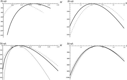
Despite the fact that we are assuming an inﬁnite-sites mutation model [Wang and Hey (2010) used a Jukes– Cantor (Jukes and Cantor 1969) model], the results from the pairwise analysis on the full data (Table 1) agree well with those obtained by Wang and Hey (2010). As expected, our maximum-likelihood estimate (MLE) ofNe(5.5 ·106) falls in between theNeestimates obtained by Wang and Hey (2010, Table 7) for the ancestral population (3.1·106_{) and} D. simulans (5.9·106_{) (note that Wang and Hey 2010}_ﬁ_t a slightly more complex history with separateNeparameters for each species). Likewise, estimates ofMandTagree well with the results of Wang and Hey (2010). The trimming of back mutations and topologically incongruent mutations led to a slight decrease inNeand increased estimates ofMin the pairwise analysis. This effect was more pronounced in the triplet analysis; in particular, the MLE for Mwas threefold higher than the estimate of Wang and Hey (2010) (Table 1). Furthermore (and perhaps unexpectedly) we found no in-crease in power in the triplet analysis (Figure 4). To inves-tigate this further, we repeated these analyses on simulated data generated using ms (Hudson 2002) under the IM his-tory estimated for the twoDrosophilaspecies,i.e., using the MLE obtained from the pairwise analysis on the trimmed data (Table 1). In contrast to the Drosophilaanalyses, we found no bias in parameter estimates and higher power to estimateMandTin triplet compared to pairwise analyses of these simulated data (Figure 4). This suggests that the dif-ferences between pairwise and triplet analyses seen in the

Drosophila example result from violations of the inﬁ nite-sites mutation model rather than from an inherent bias of our method. An obvious interpretation is that the use of

shared derived mutations to infer the topology at each locus in the triplet analysis makes our method sensitive to misin-ference of ancestral states resulting from backmutations on the outgroup branch. In other words, mispolarized muta-tions artificially inflate the proportion of loci with incongru-ent topologies and hence the estimate of M. As a simple check, we can ask what the expected frequencies of congru-ent, incongrucongru-ent, and topologically uninformative loci are (these can be derived from the GF analogous to Equation 16; see File S1). Given the MLE for trimmed pairwise and triplet analysis (Table 1), we expect 2.1% incongruent and 15.7% topologically uninformative loci on the basis of the pairwise results and 2.6% incongruent and 19.3% uninfor-mative loci on the basis of the triplet results. However, the observed frequencies in the data set are 6.2% and 18.8% for topologically incongruent and uninformative loci, respec-tively. This confirms that there is an apparent (and likely artificial) excess of incongruent topologies in the data that explains the bias seen the triplet MLEs. While this illustrates the problems of assuming infinite-sites mutations when dealing with old divergence events, it is actually surprising how little effect ignoring back mutations had in this case, considering the large distance between in- and outgroup.

We also analyzed triplet data simulated under the re-verse sampling scheme (two individuals from the species/ population receiving migrants). The GF for this is slightly more complicated and is derived in File S1. The power to estimateMin this case increases substantially when analyz-ing triplets (Figure 4). This is expected given that most migration events will result in incongruent genealogies with relatively long internal branches.

Discussion

The GF framework provides a general method to derive likelihoods under a variety of models that include migration, changes in population structure, and recombination and applies to arbitrary sample sizes. Here our aim is to set out the method and show that it can be implemented for indeﬁnitely large numbers of loci. So, we have focused on small samples for simplicity. Assuming that populations are exchangeable in size and rate of migration reduces both the number of parameters to be estimated and the number of conﬁgurations to track. In the case of the symmetric IM model, we do not need to distinguish the two demes, which

Table 1 Population parameters estimated forD. melanogaster–D. simulansusing 26,141 loci (data from (Wang and Hey 2010)

Data set u(Ne) M¼4Nm T(t) logL

Pair, full data 1.85 (5.52·106₎ _0.051 _{2.70 (2.98}_·₁₀6₎ ₂_93,466

Pair, trimmeda 1.51 (4.72·106₎ _0.093 _{3.34 (}_3.15_·₁₀6₎ ₂_65,717

Triplet, trimmeda 1.40 (4.37·106₎ _0.174 _{3.34 (2.92}_·₁₀6₎ ₂_149,556

Pair, simulated 1.53 (4.79·106₎ _0.098 _{3.24 (3.10}_·₁₀6₎ ₂_65,619

Triplet, simulated 1.51 (4.72·106₎ _0.092 _{3.29 (3.11}_·₁₀6₎ ₂_151,483

Absolute values are in parentheses. MLEs forMandtin the pairwise analysis agree well with the results of Wang and Hey (2010) who estimatedt¼3.04 andM¼0.059 (after correction for differences in scalingM). Theﬁltering necessary to satisfy the inﬁnite-sites model leads to a decrease in the estimate ofNeand an increase inM. The last two rows show parameters estimated from data simulated using the MLE from the pairwise analysis (boldface type).

a_{Trimmed refers to shortening each locus to a}_ﬁ_{xed outgroup divergence and removing back mutations and topologically incongruent mutations.}

(9)

halves the number of sample configurations. At the opposite extreme, under a highly asymmetric model with unidirec-tional migration (as in theDrosophilaexample above), each lineage in the receiving population can be affected by only a single migration event at most, which also greatly simpli-fies the problem. More generally, although it is possible to calculate the GF for fairly complex problems (up to six genes in the IM model, say), it is harder to extract useful informa-tion from it. Thus, while we can readilyfind the properties of chosen summary statistics (for example, the number of segregating sites), tabulating the probability of all observed mutational configurations is limited by their sheer number, rather than by the difficulty offinding the GF itself. These computational issues are explored in File S1, using auto-mated recursions for the IM model with three genes.

Our GF approach is moreflexible than those of Wang and Hey (2010) and Hobolthet al.(2011) in two ways. First, the recursions for a given data set can be simplified by dropping terms that are incompatible with the observed mutational pattern. This strategy is closely related to importance sam-pling schemes (e.g., Griffiths and Tavaré 1994). Thus, instead of summing over all possible topologies, the calculation is

reduced to histories that are possible, given the data. For a sample with a fully resolved topology, the total number of terms is given by the number of conﬁgurations due to migra-tion, so that for n ¼ 4 and 6 there are only 28 and 124 conﬁgurations, respectively. Thus, solutions at least for sym-metric cases are feasible. Second, other processes, such as recombination or changes in population size, can easily be incorporated into the GF framework. Since, under the IM model, genealogies involving migration events tend to be shorter and thus more likely to be shared between linked loci, incorporating recombination should improve inference.

Given that species may diverge gradually in space and/or ecology, it makes sense to model population separation as an explicit process, rather than an instantaneous event, followed by constant geneflow. We must distinguish here between our GF method, which calculates an average over exponentially distributed split times, and more general models that allow varying rates of gene flow. We follow the IM model in assuming that populations split abruptly and that subse-quently, genesflow at a constant rate. Our initial assumption of an exponential distribution of separation times (with rateL) can be viewed either as a technical ruse to allow us

Figure 4 Proﬁle log-likelihood curves forM(left plots) andu(right plots) for pairwise (dashed lines) and triplet analyses (thick solid lines) calculated from 26,141 loci for D. melanogasterandD. simulans(Wang and Hey 2010) (top row) and simulated data under an IM model with migration from D. simulanstoD. melanogaster(bottom row). Analysis of theDrosophiladata suggests an apparent bias of the triplet MLE ofMand no improvement in power. Comparison with data simulated under the same history (using the MLE obtained in the pairwise analysis, see Table 1) shows no bias and tighter log-likelihood for the triplet analyses as expected. The improvement in power when adding a third individual is greater if this is sampled from the species receiving migrants [i.e., the reverse sampling as in theDrosophilaexample (thin solid lines)].

(10)

to recover the distribution at a specific time,T, by taking an inverse Laplace transform or, in Bayesian terms, as expressing our prior beliefs about T. In reality, gene flow is likely to decrease gradually as populations diverge, and we can imag-ine a variety of models for the way rates of gene flow vary through time. However, even with large data sets there may be little power to detect changes in the rate of gene flow (Becquet and Przeworski 2009); the question of whether rates of geneflow vary across loci as a result of selection is yet more challenging, but crucial to identifying genes respon-sible for reproductive isolation (e.g., Machado 2002).

Yang (2010) recently introduced a model that is related to both approaches just described. This assumes that popu-lations separate suddenly, with no subsequent geneflow, but that the split time varies across loci, following a beta distri-bution—which can be regarded as an approximation to a biologically feasible model in which migration causes var-iation in coalescence time across loci. This is related to, but different from, our assumption of an exponential rate,L, of separation times. If, following Yang (2010), we assumed exponentially distributed split times across loci, we would fix L to find the probability of mutational configurations. On the other hand, if we assumed a definite separation time

T, we would take the inverse Laplace transform at T and calculate the probabilities from that. If we then averaged the multilocus likelihood over a prior distribution of T, we would get a quite different result from that yielded by Yang’s (2010) procedure.

As our application to the Drosophiladata demonstrates, the GF method outlined here provides an efficient way to calculate and maximize the joint likelihood of divergence parameters from very many nonrecombining blocks of se-quence for topologically informative samples. Not only do triplet samples (as opposed to pairs) give better information about branch lengths but also, more importantly, the joint distribution of topologies and branch lengths provides qual-itatively new information about historical parameters. As our simulation example demonstrates, dependent on the sampling scheme, this substantially increases power. Our analytic solutions have three key advantages over previous methods. First, the probabilities of mutational confi gura-tions need to be tabulated only once, so in contrast to sim-ulation-based methods computation time does not increase with the number of loci and an indefinite number of loci can be analyzed. Second, derivatives can be used to maximize the joint log-likelihood, which greatly speeds up calcula-tions. Thus our computation takes a fraction of the time of, for example, an IMa analysis (Hey and Nielsen 2004) on a handful of loci and is also more efficient than the numerical method of Wang and Hey (2010) (Y. Wang, per-sonal communication). Finally, the GF method allows us to separate topology and branch length information, which provides a way to incorporate additional sources of informa-tion. For example, topology information contained in the patterns of shared derived indels could be included without the need to model indel evolution explicitly.

In practice, however, our method is currently limited to the infinite-sites mutation model and thus can deal with only relatively recent divergence events for which close outgroups are available. However, it is encouraging how small the bias resulting from assuming infinite-sites muta-tions is in theDrosophilaexample, despite the considerable divergence of the outgroup. Fortunately, researchers are commonly interested infitting IM histories to sister taxa or populations that have diverged much more recently than the

Drosophila species analyzed here (and for which more

closely related outgroups are available). The use of multiple outgroups to correct for misinferred ancestral states should also help to overcome this problem. Another limitation is that the GF can be used to ﬁnd exact solutions only if the number of mutations per genealogical branch is relatively small (e.g., the most diverse locus in the trimmedDrosophila

data set contained 26 mutations). For much larger numbers of mutations per block, numerical calculations, which in-volve ﬁnding the coefﬁcients in a series expansion, become unfeasible. Although it may be possible to use a Gaussian approximation in this case, the assumption of no recombi-nation within blocks restricts our and related methods (Hey and Nielsen 2004; Wang and Hey 2010) to short blocks of sequence anyway, so this may not be relevant in practice.

Implementing efficient inference schemes for biologically realistic histories clearly requires further work. For instance, it would be worthwhile to extend our inference scheme to the general IM model (i.e., allowing for asymmetric migra-tion in both direcmigra-tions and different populamigra-tion sizes) and more realistic mutation models and incorporate recombina-tion explicitly. In contrast, the catastrophic increase of pos-sible sample and mutational configurations with the number of individuals frustrates full results for large numbers of individuals. Nevertheless, full results for small but topolog-ically informative samples under a range of models of struc-ture and history should be of considerable interest for at least three reasons: first, although thorough investigations of the trade-offs of various sampling schemes are lacking, it is clear that in general replication across loci is far more profitable than analyzing a few loci sampled from a large number of individuals (Felsenstein 1992; Li and Durbin 2011). Second, minimal sampling in terms of individuals reflects the practical limitations of current sequencing tech-nologies. While massively paralleled sequencing has made it affordable to sequence small numbers of genomes in any organism, obtaining multilocus sequence data for many indi-viduals remains challenging in nonmodel organisms. Finally, under a wide range of models of population structure, large samples quickly coalesce down to a few lineages that dom-inate their genealogical history, allowing a separation of timescales to be applied (Wakeley 2009). Thus, we envisage that new analytic solutions of simple cases, such as those derived here for the total number of mutations and topolog-ical probabilities of triplets under the IM model, will provide a guide to the development of approximate methods

(11)

(involving importance sampling and summary statistics) with wide applicability.

Acknowledgments

We thank Yong Wang and Jody Hey for sharing the Dro-sophila data set. We also thank two anonymous reviewers and Jerome Kelleher for thoughtful comments on earlier versions of this manuscript. This work was supported by a grant from the European Research Council (250152) (to N.B.) and a grant from the United Kingdom Natural Envi-ronment Research Council (NE/I020288/1) (to K.L.).

Literature Cited

Becquet, C., and M. Przeworski, 2009 Learning about modes of speciation from computational approaches. Evolution 63(10): 2547–2562.

Felsenstein, J., 1992 Estimating effective population size from samples of sequences: inefﬁciency of pairwise and segregating sites as compared to phylogenetic estimates. Genet. Res. 59: 139–147.

Grifﬁths, R. C., 1981a The number of heterozygous loci between two randomly chosen completely linked sequences of loci in two subdivided population models. J. Math. Biol. 12: 251_–261. Grif_ﬁths, R. C., 1981b Transient distribution of the number of

segrating sites in a neutral in_ﬁnite-sites model with no recom-bination. J. Appl. Probab. 18: 42_–51.

Grif_ﬁths, R. C., 1991 The two-locus ancestral graph, pp. 100_–117 in, editors, Selected Proceedings of the Symposium of Applied Probability, edited by I. V. Basawa and R. I. Taylor. Institute of Mathematical Statistics, Haywards, CA.

Grifﬁths, R. C., and S. Tavaré, 1994 Sampling theory for neutral alleles in a varying environment. Philos. Trans. R. Soc. Lond. B Biol. Sci. 344(1310): 403–410.

Herbots, H., 1997 The structured coalescent, pp. 231–255 in Progress in Population Genetics and Human Evolution(IMA Vol-umes in Mathematics and Its Applications, No. 87), edited by P. Donelly and S. Tavare. Springer-Verlag, Berlin/Heidelberg, Germany/New York.

Hey, J., and R. Nielsen, 2004 Multilocus methods for estimating population sizes, migration rates and divergence time, with

ap-plications to the divergence of Drosophila pseudoobscura and D. persimilis. Genetics 167: 747–760.

Hobolth, A., L. N. Andersen, and T. Mailund, 2011 On computing the coalescent time density in an isolation-with-migration model with few samples. Genetics 187: 1241–1243.

Hudson, R. R., 2002 Generating samples under a Wright-Fisher neutral model of genetic variation. Bioinformatics 18: 337–338. Jenkins, P. A., 2008 Importance sampling on the coalescent with

recombination. Ph.D. Thesis, Oxford University, Oxford. Jukes, T. H., and C. R. Cantor, 1969 Evolution of protein

mole-cules, pp. 21_–123 inMammalian Protein Metabolism, edited by H. N. Munro. Academic Press, New York.

Latter, B. D. H., 1973 The island model of population differenti-ation: a general solution. Genetics 73: 147_–157.

Li, H., and R. Durbin, 2011 Inference of human population history from individual whole-genome sequences. Nature 475(7357): 493–496.

Machado, C. A., 2002 Inferring the history of speciation from multilocus DNA sequence data: the case of Drosophila pseu-doobscuraand close relatives. Mol. Biol. Evol. 19: 472–488. Simonsen, K. L., and G. A. Churchill, 1997 A Markov chain model

of coalescence with recombination. Theor. Popul. Biol. 52: 43– 59.

Slatkin, M., and J. L. Pollack, 2006 The concordance of gene trees and species trees at two linked loci. Genetics 172: 1979–1984. Takahata, N., Y. Satta, and J. Klein, 1995 Divergence time and population size in the lineage leading to modern humans. Theor. Popul. Biol. 48: 198–221.

Wakeley, J., 1996 Pairwise differences under a general model of subdivision. J. Genet. 75(1): 81_–89.

Wakeley, J., 2009 Coalescent Theory. Roberts & Co., Greenwood Village, CO.

Wang, Y., and J. Hey, 2010 Estimating divergence parameters with small samples from a large number of loci. Genetics 184: 363–373.

Wilkinson-Herbots, H. M., 2008 The distribution of the coales-cence time and the number of pairwise nucleotide differences in the“isolation with migration”model. Theor. Popul. Biol. 73(2): 277–288.

Yang, Z., 2002 Likelihood and Bayes estimation of ancestral pop-ulation sizes in hominoids using data from multiple loci. Genet-ics 162: 1811–1823.

Yang, Z., 2010 A likelihood ratio test of speciation with geneﬂow using genomic data. Genome Biol. Evol. 2: 200–211.

Communicating editor: Y. S. Song

(12)

GENETICS

Supporting Information

http://www.genetics.org/content/suppl/2011/09/07/genetics.111.129569.DC1

A General Method for Calculating Likelihoods Under

the Coalescent Process

K. Lohse, R. J. Harrison, and N. H. Barton

(13)

Supplementary Information

It is easiest to view this document in Mathematica or MathPlayer (available as a free download at http://www. wolfram.com/producs/-player/).

1. Automation for the IM model: Three genes in two demes

1.1 Set up

ã Notation

Lineages are labelled by the set of genes to which they are ancestral. Thus, lineages at the tips are ancestral to a single gene, and are labelled 8a<, 8b<, …. A deme containing lineages 8b< and 8c< is denoted 88b<, 8c<<, and two demes - one containing lineage 8a< and the other containing 8b< and 8c< - is denoted 888a<<, 88b<, 8c<<<. If populations can split, we also need to define the ancestry of

the demes in a similar way. 88x<, 8y<< denotes two demes, ancestral to the present-day demes x and y . The single ancestral deme that

existed before the split is denoted 88x , y<<. Note that a single lineage must be ancestral to every gene, and a single deme must be

ancestral to every present-day deme. Thus, the content of the lists that define the genealogy and the population phylogeny stays the same - only the nesting changes.

The generating function has the form GF@Ω, 888a<<, 88b<, 8c<<<, M , 88x<, 8y<<, LD. Ω@ 8a<D corresponds to branch 8a<,

which is ancestral to a ; L@ 8x , y<D is the split rate of population 8x , y<. M =4 N m is the scaled migration rate

In the text, this is denoted more compactly as Ψ@a , b \cD. tidyNotation[Ψ] gives something like this notation, to make the output more

readable.

ã Solving the recursions

This procedure is simple, but not very efficient given that it does not exploit all the symmetries, which can drastically reduce the number of equations needed. However, this part is extremely fast relative to later steps.

makeAllEqns automates the recursions for the IM model. Here we assume a sampling configuartion {a/b,c}.

eqs=makeAllEqns@GF@Ω,888a<<,88b<,8c<<<, M ,88x<,8y<<,LDD; vars=GetVars@eqsD

8GF@Ω,888a<,8b , c<<<, M ,88x , y<<,LD, GF@Ω,888b<,8a , c<<<, M ,88x , y<<,LD, GF@Ω,888c<,8a , b<<<, M ,88x , y<<,LD, GF@Ω,888a<,8b<,8c<<<, M ,88x , y<<,LD,

GF@Ω,88<,88a<,8b , c<<<, M ,88x<,8y<<,LD, GF@Ω,88<,88b<,8a , c<<<, M ,88x<,8y<<,LD, GF@Ω,88<,88c<,8a , b<<<, M ,88x<,8y<<,LD, GF@Ω,88<,88a<,8b<,8c<<<, M ,88x<,8y<<,LD, GF@Ω,888a<<,88b , c<<<, M ,88x<,8y<<,LD, GF@Ω,888a<<,88b<,8c<<<, M ,88x<,8y<<,LD, GF@Ω,888b<<,88a , c<<<, M ,88x<,8y<<,LD, GF@Ω,888b<<,88a<,8c<<<, M ,88x<,8y<<,LD, GF@Ω,888c<<,88a , b<<<, M ,88x<,8y<<,LD, GF@Ω,888c<<,88a<,8b<<<, M ,88x<,8y<<,LD, GF@Ω,888a , b<<,88c<<<, M ,88x<,8y<<,LD, GF@Ω,888a , c<<,88b<<<, M ,88x<,8y<<,LD, GF@Ω,888b , c<<,88a<<<, M ,88x<,8y<<,LD, GF@Ω,888a<,8b<<,88c<<<, M ,88x<,8y<<,LD, GF@Ω,888a<,8c<<,88b<<<, M ,88x<,8y<<, LD, GF@Ω,888a<,8b , c<<,8<<, M ,88x<,8y<<, LD, GF@Ω,888b<,8c<<,88a<<<, M ,88x<,8y<<, LD, GF@Ω,888b<,8a , c<<,8<<, M ,88x<,8y<<, LD, GF@Ω,888c<,8a , b<<,8<<, M ,88x<,8y<<,LD, GF@Ω,888a<,8b<,8c<<,8<<, M ,88x<,8y<<,LD<

(14)

eqs1=selectEqns@eqs , 81 , All<D;

soln1 = Solve@eqs1 , First eqs1D@@1DD

:GF@Ω,888a<,8b , c<<<, M ,88x , y<<, LD®

-1

-1- Ω@8a<D- Ω@8b , c<D ,

GF@Ω,888b<,8a , c<<<, M ,88x , y<<,LD®

-1

-1- Ω@8b<D- Ω@8a , c<D ,

GF@Ω,888c<,8a , b<<<, M ,88x , y<<,LD®

-1

-1- Ω@8c<D- Ω@8a , b<D ,

GF@Ω,888a<,8b<,8c<<<, M ,88x , y<<, LD®

1 HH3+ Ω@8a<D+ Ω@8b<D+ Ω@8c<DL H1+ Ω@8c<D+ Ω@8a , b<DLL -1 HH3+ Ω@8a<D+ Ω@8b<D+ Ω@8c<DL H-1- Ω@8b<D- Ω@8a , c<DLL

-1 HH3+ Ω@8a<D+ Ω@8b<D+ Ω@8c<DL H-1- Ω@8a<D- Ω@8b , c<DLL>

We then choose those that involve 2 genes in 2 demes:

eqs2=selectEqns@eqs , 82 , 2<D;

soln2=Solve@eqs2 , First eqs2DP1T;

This needs to be simplified, by using the solutions for all the 1-deme cases (stored in soln1). This is the solution for all configurations with two genes in two demes. Note that this is inefficient: there are 12 configurations in general, but only three kinds for the symmetric model (where both demes have equal popultaion size and migration is symmetric) - the genes can be in the same deme or different demes.

These are the solutions for two genes with two demes, given in the "tidy notation". Ψ_8<_,₉₈_a_<_,₉_{b , c}₌₌ denotes an empty deme, and a deme

containing two lineages - one ancestral to 8a<, the other to 8b , c<.

soln2Simp=soln2. soln1Simplify ;

soln2Simp. tidyNotation@ΨD .9Ω₈x_ , y_<:> ΩL- ΩComplement A9a , b , c=,8x , y<E,L8x<,8y<® L= Simplify

9Ψ_8<_,₉₈_a_<_,₉_{b , c}₌₌ ®IM+ L +2 M L + L2+H1+M+2 LL ΩL + ΩL

2M

IH1+ ΩLL IM+ L +2 M L + L 2

+H1+2 M +2 LLΩL + ΩL 2_MM

, Ψ_8<_,₉₉_b₌_,₈_{a , c}_<=®

IM+ L +2 M L + L2+H1+M+2 LL ΩL + ΩL 2_{M IH}

1+ ΩLL IM+ L +2 M L + L 2

+H1+2 M +2 LL ΩL+ ΩL 2_MM

,

Ψ_8<_,₉₈_c_<_,₉_{a , b}₌₌®IM+ L +2 M L + L2+H1+M+2 LLΩL+ ΩL

2M

, Ψ₈₈_a_<<_,₉₉_{b , c}₌₌ ®

IM+ L +2 M L + L2+HM+ LLΩLM IH1+ ΩLL IM+ L +2 M L + L 2

+H1+2 M+2 LLΩL+ ΩL

2_MM

,

Ψ₉₉_b₌₌_,₈₈_{a , c}_<< ®IM+ L +2 M L + L2+HM+ LLΩLM

, Ψ₈₈_c_<<_,₉₉_{a , b}₌₌ ®

2_MM

,

Ψ₉₉_{a , b}₌₌_,₈₈_c_<< ®IM+ L +2 M L + L2+HM+ LLΩLM

, Ψ₈₈_{a , c}_<<_,₉₉_b₌₌ ®

2_MM

,

Ψ₉₉_{b , c}₌₌_,₈₈_a_<< ®IM+ L +2 M L + L2+HM+ LLΩLM

, Ψ₉₈_a_<_,₉_{b , c}₌₌_,_8<®

1+ ΩLL IM+ L +2 M L + L 2

+H1+2 M +2 LL ΩL+ ΩL 2_MM

,

Ψ₉₉_b₌_,₈_{a , c}_<=_,_8<®IM+ L +2 M L + L2+H1+M+2 LLΩL+ ΩL

2_M

, Ψ₉₈_c_<_,₉_{a , b}₌₌_,_8<®

1+ ΩLL IM+ L +2 M L + L 2

+H1+2 M +2 LL ΩL+ ΩL

2_MM=

We have rewritten this in terms of Ω_L, which refers to the sum of the Ω's for the two lineages involved.

(15)

eqs3=selectEqns@eqs , 82 , 3<D;

soln3=Solve@eqs3 , First eqs3DP1T;

soln3Simp=soln3. soln1. soln2Simp ;

As a check, if we set Ω®0, the GF is always 1, independent of L:

soln3Simp.8Ω@_D®0<  Simplify

8GF@Ω,88<,88a<,8b<,8c<<<, M ,88x<,8y<<,LD®1 ,

GF@Ω,888a<<,88b<,8c<<<, M ,88x<,8y<<, LD®1 , GF@Ω,888b<<,88a<,8c<<<, M ,88x<,8y<<,LD®1 , GF@Ω,888c<<,88a<,8b<<<, M ,88x<,8y<<, LD®1 , GF@Ω,888a<,8b<<,88c<<<, M ,88x<,8y<<,LD®1 , GF@Ω,888a<,8c<<,88b<<<, M ,88x<,8y<<, LD®1 , GF@Ω,888b<,8c<<,88a<<<, M ,88x<,8y<<,LD®1 , GF@Ω,888a<,8b<,8c<<,8<<, M ,88x<,8y<<,LD®1<

1.2 Sumaries for exponentially distributed split times

ã The total length of the genealogy

A relatively simple expression can be obtained for the distribution of total length of the genealogy, T =t8a< +t8b< +…, for a given L by

setting all the Ω to be the same, so that Ψ = E@expH- ΩTL D

(16)

ss=soln3Simp.Ω@_D® Ω. tidyNotation@ΨD .L₈x<,8y<® L Simplify

9Ψ_8<_,₉₈_a_<_,₉_b₌_,₈_c_<= ®IL4+5 L3 H1+2 ΩL+ L2 I7+36 Ω +37 Ω2M+6 Ω I1+6 Ω +11 Ω2+6 Ω3M+ L I3+32 Ω +85 Ω2+60 Ω3M+M2 I3+4 L2+9 Ω +6 Ω2+2 L H4+7 ΩLM+

M I4 L3+ L2 H14+27 ΩL+ L I13+56 Ω +53Ω2M+3I1+7 Ω +14 Ω2+8 Ω3MMM

IH1+ ΩL H1+2 ΩL IM+ L +2 M L + L2₊₂ _{Ω +}_{4 M} _{Ω +}₄ _{L Ω +} ₄ _Ω2M

I3+ L2+12 Ω +9 Ω2+ L H4+6 ΩL+M H3+2 L +6 ΩLMM, Ψ₈₈_a_<<_,₉₉_b₌_,₈_c_<= ®IM2 I3+4 L2+9 Ω +6 Ω2+2 L H4+7 ΩLM+

M I4 L3+3H1+ ΩL H1+2 ΩL2+ L2 H14+23ΩL+ L I13+46 Ω +37 Ω2MM+

L IL3+ L2 H5+8 ΩL+ L I7+26 Ω +21 Ω2M+3I1+6 Ω +11 Ω2+6 Ω3MMM

IH1+ ΩL H1+2 ΩL IM+ L +2 M L + L2₊₂ _{Ω +}_{4 M} _{Ω +}₄ _{L Ω +} ₄ _Ω2M

I3+ L2+12 Ω +9 Ω2+ L H4+6 ΩL+M H3+2 L +6 ΩLMM, Ψ₉₉_b₌₌_,₈₈_a_<_,₈_c_<< ®IM2 I3+4 L2+9 Ω +6 Ω2+2 L H4+7 ΩLM+

IH1+ ΩL H1+2 ΩL IM+ L +2 M L + L2+2 Ω +4 M Ω +4 L Ω + 4 Ω2M

I3+ L2₊₁₂ _{Ω +}₉ _Ω2_{+ L} H₄₊₆ _ΩL₊_M H₃₊₂ _{L +}₆ _ΩLMM_,

Ψ₈₈_c_<<_,₉₈_a_<_,₉_b₌₌ ®IM2 I3+4 L2+9 Ω +6 Ω2+2 L H4+7 ΩLM+

Ψ₉₈_a_<_,₉_b₌₌_,₈₈_c_<< ®IM2 I3+4 L2+9 Ω +6 Ω2+2 L H4+7 ΩLM+

Ψ₈₈_a_<_,₈_c_<<_,₉₉_b₌₌ ®IM2 I₃₊₄ _L2₊₉ _{Ω +}₆ _Ω2₊₂ _L H₄₊₇ _ΩLM₊

M I4 L3₊₃H₁_{+ Ω}L H₁₊₂ _ΩL2_{+ L}2 H₁₄₊₂₃_ΩL_{+ L} I₁₃₊₄₆ _{Ω +}₃₇ _Ω2MM₊

I3+ L2+12 Ω +9 Ω2+ L H4+6 ΩL+M H3+2 L +6 ΩLMM, Ψ₉₉_b₌_,₈_c_<=_,₈₈_a_<< ®IM2 I₃₊₄ _L2₊₉ _{Ω +}₆ _Ω2₊₂ _L H₄₊₇ _ΩLM₊

M I4 L3₊₃H₁_{+ Ω}L H₁₊₂ _ΩL2_{+ L}2 H₁₄₊₂₃_ΩL_{+ L} I₁₃₊₄₆ _{Ω +}₃₇ _Ω2MM₊

I3+ L2+12 Ω +9 Ω2+ L H4+6 ΩL+M H3+2 L +6 ΩLMM,

Ψ₉₈_a_<_,₉_b₌_,₈_c_<=_,_8< ®IL4₊₅ _L3H₁₊₂ _ΩL_{+ L}2 I₇₊₃₆ _{Ω +}₃₇ _Ω2M₊₆ _ΩI₁₊₆ _{Ω +}₁₁ _Ω2₊₆ _Ω3M₊

L I3+32 Ω +85 Ω2₊₆₀ _Ω3M₊_M2 I₃₊₄ _L2₊₉ _{Ω +}₆ _Ω2₊₂ _L H₄₊₇ _ΩLM₊

M I4 L3+ L2 H14+27 ΩL+ L I13+56 Ω +53Ω2M+3I1+7 Ω +14 Ω2+8 Ω3MMM

I3+ L2+12 Ω +9 Ω2+ L H4+6 ΩL+M H3+2 L +6 ΩLMM=