Estimating Modifying Effect of Age on Genetic and Environmental Variance Components in Twin Models

| INVESTIGATION

Estimating Modifying Effect of Age on Genetic and

Environmental Variance Components in

Twin Models

Liang He,*,†,1_{Mikko J. Sillanpää,}‡,§_{Karri Silventoinen,* Jaakko Kaprio,*},_**,††_{and Janne Pitkäniemi*},‡‡ *Department of Public Health, Faculty of Medicine, University of Helsinki FIN-00014 Helsinki, Finland,††Institute for Molecular Medicine Finland FIMM, University of Helsinki, FIN-00290 Helsinki, Finland,†Biodemography of Aging Research Unit, Social Science Research Institute, Duke University, Durham, North Carolina 27708,‡Department of Mathematical Sciences, University of Oulu, FIN-90014 Oulu, Finland,§Biocenter Oulu, FIN-90014 Oulu, Finland, **National Institute for Health and Welfare, FIN-00300 Helsinki, Finland, and‡‡Finnish Cancer Registry, Institute for Statistical and Epidemiological Cancer Research, FIN-00130 Helsinki, Finland ORCID ID: 0000-0002-3716-2455 (J.K.)

ABSTRACTTwin studies have been adopted for decades to disentangle the relative genetic and environmental contributions for a wide range of traits. However, heritability estimation based on the classical twin models does not take into account dynamic behavior of the variance components over age. Varying variance of the genetic component over age can imply the existence of gene– environment (G3 E) interactions that general genome-wide association studies (GWAS) fail to capture, which may lead to the inconsistency of heritability estimates between twin design and GWAS. Existing parametricG3Einteraction models for twin studies are limited by assuming a linear or quadratic form of the variance curves with respect to a moderator that can, however, be overly restricted in reality. Here we propose spline-based approaches to explore the variance curves of the genetic and environmental components. We choose the additive genetic, common, and unique environmental variance components (ACE) model as the starting point. We treat the component variances as variance functions with respect to age modeled by B-splines or P-splines. We develop an empirical Bayes method to estimate the variance curves together with their confidence bands and provide an R package for public use. Our simulations demonstrate that the proposed methods accurately capture dynamic behavior of the component variances in terms of mean square errors with a data set of.10,000 twin pairs. Using the proposed methods as an alternative and major extension to the classical twin models, our analyses with a large-scale Finnish twin data set (19,510 MZ twins and 27,312 DZ same-sex twins) discover that the variances of the A, C, and E components for body mass index (BMI) change substantially across life span in different patterns and the heritability of BMI drops to 50% after middle age. The results further indicate that the decline of heritability is due to increasing unique environmental variance, which provides more insights into age-specific heritability of BMI and evidence ofG3E interactions. Thesefindings highlight the fundamental importance and implication of the proposed models in facilitating twin studies to investigate the heritability specific to age and other modifying factors.

KEYWORDStwin models; penalized B-splines; age-specific heritability; empirical Bayes predictor; body mass index

T

Estimation methods and software such as structural equation modeling (SEM) based on the classical twin models consist-ing of additive genetic, common, and unshared environmen-tal effects have been well established and extensively adopted (Rijsdijk and Sham 2002). Extensions for longitudinal data or time-to-event phenotypes based on the classical twin mod-els have been proposed (Boomsma et al.1989; Pitkäniemi et al. 2007). Nevertheless, one of the major issues posing potential challenge is that many twin data sets contain indi-viduals across a wide range of age and the variances of Copyright © 2016 by the Genetics Society of America

doi: 10.1534/genetics.115.183905

Manuscript received October 20, 2015; accepted for publication February 6, 2016; published Early Online February 10, 2016.

genetic and environmental components for many complex traits such as body mass index (BMI) and height change over age (Lajunen et al.2009; Elkset al.2012) or birth cohorts (Silventoinenet al.2000). For example, the variances of ge-netic and environmental components and thus the heritabil-ity of BMI have been found to diverge with age in a Finnish study of adolescent twins (Lajunenet al.2009) and another of adolescents and young adults (Ortega-Alonsoet al.2012), implying that potential gene–environment (G 3E) interac-tions play a notable role in these complex traits. During child-hood when a twin pair is raised in a similar environment, the common environmental effects may be present in early child-hood when children are dependent on their parents and then drop after midchildhood when they start to get more inde-pendence (Silventoinen et al.2009). Unfortunately, relying on the classical twin models in these cases may lead to sub-stantially biased results (Purcell 2002; Zyphuret al.2013). In many studies, information on age at measurements is avail-able for each twin pair, and ignoring how age potentially modifies the genetic and environmental variances would re-sult in problematic estimates especially when age is distrib-uted widely and considerably different between monozygotic (MZ) and dizygotic (DZ) twin samples.

The gap between the heritability estimated from twin studies and genome-wide association studies (GWAS), known as missing heritability, is observed for many complex traits, and so far little is known about its cause (Manolioet al.2009; Eichleret al.2010). As an example, compared with a herita-bility of from nearly 50% up to 80% estimated from different twin studies for BMI (Elkset al.2012), thus far, a meta-analysis of multiple GWAS data sets has reported that 97 genome-wide significant loci account for,3% of the variance, while all common single-nucleotide polymorphisms (SNPs) account for20% of the variance in which age has been adjusted for linearly (Lockeet al.2015) and17 million variants account for around 27% of the variance (Yang et al. 2015). While literature has suggested that the fundamental assumption of additive genetics in GWAS might be problematic (Nelsonet al. 2013), estimates of heritability from the perspective of twin design should also be refined or revised by taking into account moderators such as age. One of the causes for missing herita-bility probably lies in theG3Einteractions. Increasing var-iance of the genetic component over age implies the existence of G 3 E interactions that general GWAS are not able to capture. Hence, it would be of vital concern to explore how the genetic and environmental components evolve and to estimate the variance curves on which there is no prior infor-mation available.

Exploration of dynamics of variance components over a period of growth by partitioning the phenotypic variance and covariance with quantitative genetic models can date back to W. Atchley in the early 1980s (Atchley and Rutledge 1980; Cheverudet al.1983; Pletcher and Geyer 1999; Charmantier et al.2006). Recently, approaches such as functional GWAS (fGWAS) have been proposed to explore time-varying genetic effects of SNPs by utilizing Legendre orthogonal polynomials

and longitudinal data (Wu and Lin 2006; Daset al.2011; Li and Sillanpää 2015). Different from fGWAS and its recent developments (Das et al. 2011; Li et al. 2015), which are based on a varying-coefficient model, in the case of twin study, we aim at modeling variance functions directly. One of the solutions is to divide samples into multiple strata and to estimate the variances within each stratum (Neale and Cardon 1992). The drawbacks of this strategy include that selection of cut points for strata is often unequivocal and difficult in some scenarios and twins measured at different ages are not always in the same strata. It may result in larger uncertainty of estimates due to reduced sample sizes in each stratum. Another option is to adopt an existing parametricG3E in-teraction model proposed by Purcell in which age can be modeled by adding a moderator in a linear or quadratic form (Purcell 2002). Unfortunately, the variance curves to be esti-mated in many cases are not necessarily linear or quadratic. Their patterns can often befluctuant and dramatically change across life span as shown later in this study. A concrete para-metric model is often difficult to determine beforehand. Hence, a nonparametric approach to explore the variance curves of these components can give more realistic under-standing on the pattern of the moderating effect provided that the number of estimated parameters is not too large. Most recently, Brileyet al.(2015) introduced local struc-tural equation modeling (LOSEM), which estimatesG3E interactions using a nonparametric approach based on LOWESS and SEM.

The past two decades have seen rapid advances of employ-ing B-splines, particularly penalized B-splines (P-splines) (O’Sullivan 1986; Eilers and Marx 1996), to estimate an un-known function in the context of epidemiology. With the same advantages of the flexibility as LOSEM, P-splines can further optimally choose the best model by penalizing the smoothness and perform various hypothesis tests (Ruppert et al.2003). In this work, we propose novel twin models that choose as the starting point the standard twin model based on decomposing total variance into the variance components of additive genetics (A), common environment (C), and unique environment (E) (a.k.a. the ACE model). We gener-alize the component variances as variance functions with re-spect to age by using B-splines or P-splines in which the ACE model becomes the special case when all spline coefficients within the components share the same value. We construct Table 1 An example of the data format used for model specification

MZ twins DZ twins

Twin ID Trait Age Twin ID Trait Age

1 YMð1Þ TMð1Þ 1 YDð1Þ TDð1Þ

1 YMð2Þ 1 YDð2Þ

2 YMð3Þ TMð2Þ 2 YDð3Þ TDð2Þ

2 YMð4Þ 2 YDð4Þ

fM YMðnM21Þ TMðfMÞ fD YDðnD21Þ TDðfDÞ

expectation-maximization (EM) and Markov chain Monte Carlo (MCMC) algorithms to estimate the variance functions together with their pointwise confidence bands and construct an R pack-age based on these models. We then show through simulation studies and a real data analysis that the proposed models along with the estimation are well behaved and are capable of depict-ing a refined picture of dynamic behavior of the component variances, which provides more insights into the age-specific heritability. Our results from the analysis of a Finnish twin data set indicate that there exist remarkable age-dependent effects on all A, C, and E components for BMI and age should be taken into account when estimating the heritability of BMI.

Methods

Suppose that we have observed zero-mean normally distrib-uted quantitative phenotypic dataYM(annM31 vector) and

YD(annD31 vector) forfMð¼nM=2ÞMZ andfDð¼nD=2ÞDZ

twin pairs, respectively. The phenotypes of each twin pair are measured at the same ageTM(anfM31 vector) andTD(an

fD31 vector). An example of the observed data format is

shown in Table 1.

According to the ACE model, we have a random effect model YMðiM;jÞ¼aMðiMÞþcMðiMÞþeðiM;jÞfor the MZ twin pair iM and a modelYDðiD;jÞ¼a1DðiDÞþa2DðiD;jÞþcDðiDÞþeðiD;jÞfor the DZ twin pairiD;whereiM2 f1;. . .;fMg;iD2 f1;. . .;fDg;

and j¼1;2: Here we assume that aM N ð0; s2aÞ; a1D;a2D N ð0;0:5s2aÞ;cM;cD N ð0;s2cÞ;ande N ð0;s2eÞ; where s2

a; s2c; and s2e 2 ð0;þNÞ are the additive genetic, common, and unique environmental components, respec-tively. Thus, this model implies that the phenotypes follow the following normal distribution,

YM

YD

N0 0

; SM 0 0 SD

; (1)

where SM¼s2

a1MB þs2c1MB þs2eI (an nM3nM matrix), SD¼s2

aAþs2c1DBþs2eI(annD3nDmatrix),1MB ¼IfM512;

1D

B¼IfD512;and A¼IfD5A2;where 12¼

1 1 1 1

;A2¼

1 0:5 0:5 1

;and5represents the Kronecker product.

Estimation of variance curves using B-splines

Wefirst propose a nonparametric approach, referred to as an ACE(t) model, to estimate the variance curves of the additive genetic and common environmental components using B-splines (de Boor 1978) with a set of evenly distributed knots. We assume that the A and C variances are represented at each time point with their own parameters as follows:

s2

aðtÞ;s2cðtÞ; t¼1;. . .;T: (2) Note that at this stage we assumes2

eðtÞ ¼s 2

eto be constant over time although including an age-dependent unique envi-ronmental component can be readily extended. Instead of trying to estimate s2

aðtÞ [or s2cðtÞ] separately at each time

point, we assume that values at adjacent time points are more alike; that is, they can be described as a smooth curve over time. First, values in (2) are expressed using linear combina-tions of B-spline basis funccombina-tions as

s2 aðtÞ ¼e

PK k¼1b

A kBAkðtÞ

and

s2 cðtÞ ¼e

PL l¼1b

C lBClðtÞ;

wherebA _{2 ð2N;þNÞ}K

andbC_{2 ð2N;þNÞ}L

are the vec-tors of coefficients. We selectKandLB-spline basis functions for the A and C components, respectively. We choose the B-spline basis functionsBA_ðtÞandBC_{ðtÞwith a degreep¼2} (or an order of 3) for the following simulation and real data analyses. The degreep¼2 is probably appropriate for most traits as the variance curves of the A and C components are generally smooth and do not change sharply within a small age interval. Thus, the numbers of knots for construction of the B-splines for the A and C components areKþpþ1 and Lþpþ1:Replacing the variancess2

aands2cin the model (1) with their time-dependent counterpartss2

aðtÞands2cðtÞleads to the covariance matrices

SM¼diag

eBATMb A

512þdiag

eBCTMb C

512þs2eI;

SD¼diag

eBATDbA5A₂þ_diageBCTDbC51₂þs2 eI;

whereBA

TM;B C

TM;B A

TD;andB C

TDarefM3K;fM3L;fD3K;and fD3Ldesign matrices of the B-spline basis functions evaluated

atTM andTDfor the MZ and DZ twins and diagð:Þconverts a

vector to a diagonal matrix with the vector entries as its di-agonal elements. The model becomes the classical ACE model when the coefficients share the same value withinbAandbC; respectively. The estimates ðbcA; bcCÞ can be obtained using maximum-likelihood estimation (MLE), and the variance

curvess2

aðtÞands 2

cðtÞare estimated bysc2aðtÞ ¼e PK

k¼1bb A kBAkðtÞ

andsc2 cðtÞ ¼e

PL l¼1bb

c

lBClðtÞ:The detailed derivation of the MLE for the ACE(t) model is described in theAppendix.

The pointwise (not simultaneous) confidence bands for the ACE(t) model can be constructed from a Delta method as previously described (Rosenberg 1995; Mao and Zhao 2003). In this case, according to the Delta method the estimates sc2

aðtÞ andsc2cðtÞ at the time point tfollow nor-mal distributions with the variances approximated by d

VarðePKk¼1bb A

kBAkðtÞÞ ¼_e2 PK

k¼1bb A

kBAkðtÞ ðBAðtÞ9Hg bA

21

BA_ðtÞÞ and

d VarðePLl¼1bb

C

lBClðtÞÞ ¼e2 PL

l¼1bb c

lBClðtÞ ðBCðtÞ9Hg bC

21

BC_{ðtÞÞ; where} ~

H21is the inverse of the estimated Fisher information from the MLE (i.e., the inverse of the Hessian of the negative log-likelihood). The confidence bands can also be estimated using a bootstrap method that is more computationally intensive than the Delta method. A parametric bootstrap-ping can be performed by first generating the bootstrap phenotypesðY*

M;YD*Þbased on model (1) with the

parame-ters replaced by their estimatesðbcA;bcC;cs2

eÞandfitting the model to obtain the bootstrap replicates ðbcA*;bcC*;sc2

e*Þ from which the confidence bands at the time pointtcan be derived (Efron and Tibshirani 1994).

Stable estimation of variance curves, using penalized splines

While the estimation and implementation of the ACE(t) model are straightforward and fast, the performance of using B-splines in practice is sensitive to the selection of the number of knots. Fewer knots suffer from large uncertainty while excessive knots can lead to overfitting. A handful of procedures for automatic knot selection have been developed; however, they are generally quite complicated and computationally intensive as pointed out by Ruppertet al.(2003), especially in the context of variance curve estimation based on large-scale twin data. One preferable way is to retain abundant knots and penalize their roughness, which is described as follows.

To reduce the impact of the number of knots, we therefore propose a more stable model using P-splines (O’Sullivan

1986), which we refer to as an ACE(t)-p model. As previously shown, the number of knots in P-splines has small influence on the results and it has been suggested that at most 35– 40 knots are generally enough for all sample sizes and for all smooth functions without too many oscillations (Ruppert 2002). Wefirst parameterize the ACE model with three random effects to decompose the covariance matri-ces and write the subsequent derivations in a matrix form. Specifically, we letZ2M¼Z3M¼IfM51231;Z1D¼

ffiffiffiffiffiffiffi 0:5 p

InD; Z2D¼

ffiffiffiffiffiffiffi 0:5 p

IfD51231;andZ3D¼IfD51231so thatZ2MZ92M¼ Z3MZ93M¼1BM;Z3DZ93D¼1BD;andZ1DZ91DþZ2DZ92D¼A;where 1231¼

1 1

:According to thefirst type of parameteriza-tion proposed by Rabe-Heskethet al.(2008) and following the notation of the spline coefficients and design matri-ces in the ACE(t) model, the covariance matrimatri-ces are ex-pressed as

SM¼Z2Mdiag

eBATMb A

Z92MþZ3Mdiag

eBCTMbC

Z93Mþs2eI;

SD¼Z1Ddiag

eBATDb A

51231

Z1D9 1Z2Ddiag

eBATDb A

Z2D9

1Z3DdiageBCTDb C

Z93D1s2eI:

The approach using P-splines imposes two penalties onbAand bC_;

respectively. We add the quadratic penaltieslAbA9DAbA

andlCbC9DCbCto the log-likelihood,

ð22Þlpsps2e;bA;bC

_¼logj

SMj1YM9 SM21YM1logjSDj 1Y9DS2D1YD1lAbA9DAbA 1lCbC_9DCbC_;

whereDAandDCare the penalty matrices constructed from

differences between neighboring coefficients according to Eilers and Marx (1996) (refer to the Appendixfor the con-tents of DAand DC). The penalizing coefficients lA andlC

substantially affect the estimation results, and many strate-gies of selecting their values have been proposed, including generalized cross-validation (Craven and Wahba 1978) and Akaike’s information criterion (Akaike 1969). P-splines in Bayesian models may be implemented via variational Bayes estimation (Li and Sillanpää 2013) and MCMC methods (Crainiceanu et al. 2005). On the other hand, under a framework of a random effects model, quadratic penalty Table 2 The empirical AMSE from the ACE(t) and ACE(t)-p models

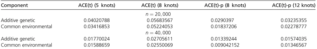
Component ACE(t) (5 knots) ACE(t) (8 knots) ACE(t)-p (8 knots) ACE(t)-p (12 knots)

n¼20;000

Additive genetic 0.04020788 0.05683567 0.0290397 0.03235355

Common environmental 0.03416853 0.05224053 0.01837206 0.02278777

n¼40;000

Additive genetic 0.01770024 0.02705611 0.01339244 0.01574035

terms can be regarded as assuming the following zero-mean normal distributions to the spline coefficients

bA _N

0;s2_bAD2_A

; bC _N

0;s2_bCD2_C

; (3)

wheres2

bA ¼1=lA;s2_bC ¼1=lC;andD2A;D2C are the

general-ized inverses of DA andDC:Expression (3) provides a

con-nection to estimation of variance components by restricted maximum likelihood (REML) in a linear mixed-model con-text (Ruppertet al.2003). To estimateb¼ ðbA;bCÞ;we fol-low a strategy adopted by Kauermann and Wegener (2011) that

first estimatesðs2

bA; s2_bCÞby using a marginal likelihood with the spline coefficientsb integrated out analytically. Based on this strategy, Krivobokova proposed a unified EM-type iterative pro-cedure (Krivobokovaet al.2008) to estimate the spline coefficients and the penalizing coefficients (now transformed to the variances of random effects in the linear mixed model) simultaneously by estimating the spline coefficients through an iterated weighted least-squares (IWLS) algorithm and employing an approximation algorithm (Breslow and Clayton 1993) to iterate between the estimation of the spline coefficients and minimization of the mar-ginal log-likelihood. More specifically, following the same spirit, the marginal likelihood in our case is

whereK~and~Lare the numbers of positive eigenvalues ofDAand

DC:By applying a Laplace approximation to the integrand of (4) with the condition ofK; LnMþnD;we obtain the22

log-likelihood

ð22Þlpsps2_e;s2_bA;s2_bC

¼K~logs2_bAþ~Llogs2_bCþlogSMb^

þYM9 S2M1 _^

bYMþlogSDb^

þYD9S2D1 _^

bYDþ d bA_9D

AbcA

s2 bA

þbdC9DCbcC

s2 bC

þlogg$b^ ;

where

gðbÞ ¼ ð1=2ÞlogjSMj þYM9 SM21YMþlogjSDj þY9DS2D1YD

þbA_9DAbA._s2

bAþbC9DCbC .

s2 bC

;

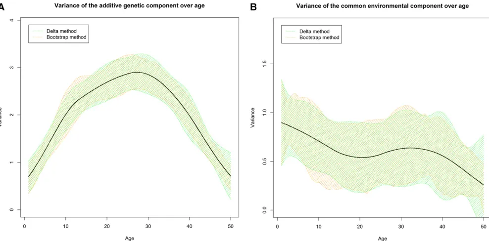
fbbgrepresents the replacement ofbatb^in the covariance matrices, and b^ is evaluated to minimize gðbÞ: Instead of Figure 2 Confidence bands constructed from the Delta and bootstrap methods for the A (shown in A) and C (shown in B) components.

Lpsp

s2

e;s2_bA;s2_bC

¼ 1

s~K bAs

~ L bC

∬ 1 jSMj1=2jSDj1=2

e2ð1=2Þ h

Y9

MS

21 MYMþY9MS

21

D YDþbA9DAbA .

s2

bAþbC9DCbC .

s2

bC i

IWLS in Krivobokovaet al.(2008), we use the limited-memory Broyden–Fletcher–Goldfarb–Shanno (L-BFGS) algorithm (Byrdet al.1995), which does not require evaluating a Hes-sian matrix explicitly. The following algorithm computes b^

together with

d s2

bA; ds2_bC

in an iterative way:

1. Give initial values to

c s2

e

ð1Þ

;ds2 bA

ð1Þ

;ds2 bC

ð1Þ

:

2. Given the values of

c s2

e

ði21Þ

; ds2 bA

ði21Þ

; ds2 bC

ði21Þ

from the

previous iteration, wefind

c

bAðiÞ_;bcCðiÞ_;

minimizinggðbÞ

by using the L-BFGS algorithm.

3. We find

c s2

e

ðiÞ

;sd2 bA ðiÞ

;ds2 bC

ðiÞ

; minimizing

ð22Þlpsp

s2

e;s2_bA;s2_bC

by using the L-BFGS algorithm with

ðbcAðiÞ_;bcCðiÞ_Þ

obtained from step 2.

4. Iterate between steps 2 and 3 until convergence.

The details of the derivation for the algorithm are given in theAppendix.

While the proposed algorithm provides a type of estimate for b;the construction of confidence intervals (C.I.’s) is far from straightforward. It has been pointed out that general bootstrap methods for the C.I.’s are overly narrow because they include only variance but not bias, which is substantial in the penalized estimation (Goeman 2010). The C.I.’s con-structed under the mixed-model framework or the posterior distribution overcome this issue (Wood 2006; Kauermann et al.2009). Recall that a best prediction (BP) for random effects in the linear mixed model is defined as the mean of the posterior distribution of random effects given data and the variances (Searleet al.2009). This does not naturally apply

to b^ as the estimated spline coefficient b^ from the above algorithm is the mode of the joint distribution of Y¼ ðYM; YDÞ and b rather than a mean b; which minimizes

the mean square error (MSE) of prediction (Searle et al. 2009). Unlike the best linear unbiased predictions (BLUPs) in the linear mixed model (Henderson 1975; Robinson 1991), the posterior meanbin our case is not a linear func-tion ofY because b is in the variance functions. Thus, we propose an MCMC method to numerically approximate the posterior distribution to obtainb;which is the estimated (or

empirical) BP of bwithðcs2

e;ds2_bA;ds2_bCÞ plugged in. From the Bayesian perspective,bis an empirical Bayes predictor ofb (Carlin and Louis 1997). Then the C.I.’s can be derived either from the conditional MSE of prediction obtained from the posterior distribution of b approximated by the MCMC method or from the marginal prediction error covariance matrix Varðb2bÞ (Booth and Hobert 1998; Skrondal and Rabe-Hesketh 2009), which can be estimated by a parametric bootstrap method. The detailed description of how to con-struct C.I.’s is given in theAppendix.

Implementation and extension

We developed an R package “ACEt”to implement the pro-posed models for public use (https://r-forge.r-project.org/

R/?group_id=2167). One of the attractive points is that both

larger sample size to obtain a reliable estimate of the vari-ances. Fortunately, as most of the matrices are sparse and block diagonal, we dramatically reduce the running time by partitioning the matrix operations twin-wisely and imple-menting the optimization functions in C++.

Our proposed models can be easily modified and extended to handle other twin models such as the AE and CE models. We can also estimate the variance curve of the unique environ-mental component together with the other components. For example, both variances in the AE model can vary over age, which we refer to as the AE(t) and AE(t)-p models. These models have been implemented and included in the ACEt R package. Their application is demonstrated in the following Finnish BMI twin study.

Data availability

The simulation data is included as an example dataset in the R package.

Results

Simulation study

We performed two simulation studies with different sample sizes to provide a rough picture of how many twin pairs are needed for reliable estimates. In these simulations, we also compared the performance among the ACE(t) models with 5 and 8 interior knots and the ACE(t)-p models with 8 and 12 interior knots. We generated phenotypic data for 5000 MZ and 5000 DZ twin pairs in thefirst simulation and twofold sample sizes in the second one, using R. Wefirst sampled a vector of

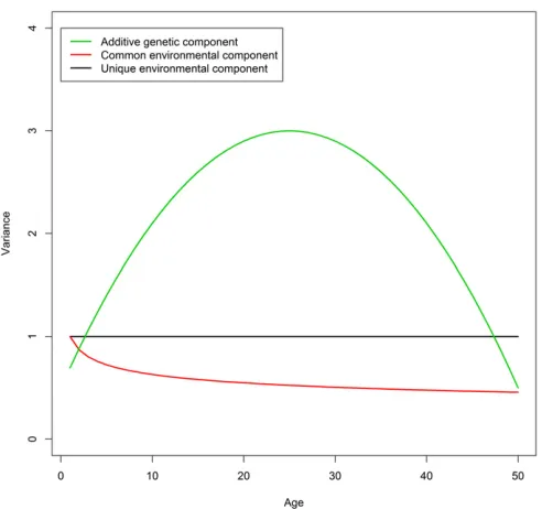
ageTfor the twin pairs that was uniformly distributed from 1 to 50. We fixed the variance of the E component at 1 and chose the following quadratic and power variance functions for the A and C components,

s2

aðTÞ ¼3210

T225 50

2

;

s2

cðTÞ ¼T20:2;

of which the shapes are depicted in Figure 1. We then simu-lated the phenotypic data by sampling from bivariate normal distributions based on Equation 1 with s2

aðTÞ and s2cðTÞ plugged into the covariance matrices. The average mean square error (AMSE), which is defined as AMSEa;c¼

1

m

Xm

i¼1

s2

a;cðtiÞ2s2ad;cðtiÞ

2

and takes into account both bias

and variance, was used to evaluate the performance of esti-mation where we chose the number of evaluated time points m¼500:In each scenario, we simulated 200 data sets and

fitted them with the proposed ACE(t) and ACE(t)-p models to calculate the AMSEs. For the ACE(t) model, we ran an addi-tional analysis to compare the confidence bands obtained from the Delta method and the bootstrap method with 200 replicates.

The results presented in Table 2 show that the AMSEs of the ACE(t) model with 8 knots are larger than those with 5 knots for both components. This suggested that 8 knots seemed excessive and could worsen the performance in terms of AMSE for the relatively smooth functions that we chose to Figure 4 The variance curves of the A and C components with the 95%

confidence bands estimated from the ACE(t) model.

investigate here. In contrast, the ACE(t)-p model had smaller AMSEs than the ACE(t) model in all scenarios, confirming its superiority of tuning the penalty term for optimal estimation as long as a sufficient number of knots is given (Ruppertet al. 2003). The ASMEs from the ACE(t)-p model with a different number of knots were more similar to each other, implying that the estimates from P-splines are much less affected by the choice of knots than those from B-splines. The smaller number of knots in the penalized spline estimator performs better in terms of AMSE, which is in accordance with a pre-vious theoreticalfinding (Claeskenset al.2009). The AMSEs decreased almost linearly with increasing sample size in all situations; however, accurate estimates still entailed thou-sands of twin pairs.

The confidence bands from the Delta method were com-parable to those from the bootstrap method for both compo-nents as plotted in Figure 2. The confidence bands estimated from the bootstrap method were less smooth due to the lim-ited number of resampling (i.e., 200 replicates), which should be adequate for the bootstrap method (Efron and Tibshirani 1994). The confidence bands from these two methods almost coincided, suggesting that the L-BFGS algo-rithm worked properly as a faster alternative to Newton’s method in this case.

A Finnish twin study of BMI

We applied both models to a twin data set retrieved from the Finnish Twin Cohort study to investigate adependent ge-netic and environmental components of BMI. The details on collection of the data were described in previous publications for older (Kaprio and Koskenvuo 2002) and younger cohorts

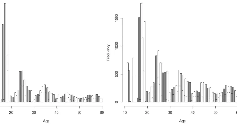
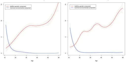
(Kaprioet al.2002). In this analysis, we included 19,510 MZ and 27,312 DZ same-sex twin individuals together with the information on age at the measurement contributed to the CODATwins project (Silventoinenet al.2015). The distribu-tions of age at the measurement among the MZ and DZ twins were widespread from 11 years to 60 years as shown in Fig-ure 3. Wefitted the data set with a linear regression on sex and age before using the residuals from the regression as the phenotypes for the analysis of variance curves. The variance curves of the genetic and common environmental compo-nents estimated from the ACE(t) (with 5 interior knots for either component) and the ACE(t)-p models (with 8 interior knots for either component) are shown in Figure 4 and Figure 5. For the ACE(t)-p model, we included more knots to ensure they were sufficient and excessive knots were affected little in terms of AMSE. The 95% pointwise confidence bands were obtained by using the bootstrap method for the ACE(t) model and the MCMC method described in the Appendix for the ACE(t)-p model. The comparable results from both models suggested that the variance of the additive genetic compo-nent started from2 at age 11 years and increased rapidly until age 35 years. After that, it leveled off for 10 years before growing again to nearly 15, except that the curve from the ACE(t)-p model had morefluctuations. In contrast, the variance of the common environmental component starting at8 at age 11 years dropped markedly before age 20 years and became almost undetectable after that. The estimated variance of the unique environmental component was 2.25. In contrast, the ACE model using the OpenMX package (Boker et al. 2011) yielded estimates of 7.384, 0.000, and 2.265 for the A, C, and E components, respectively, while the Figure 6 The variance curves after age 20 years of the A and E

compo-nents with the 95% confidence bands estimated from the AE(t) model.

AE model gave nearly the same estimates for the A and E components.

The results revealed that the common environmental fac-tor almost vanished after age 20 years, but the growth of the additive genetic factor might be attributed to an increasing unique environmental variance that was assumed to be con-stant in the ACE(t) and ACE(t)-p models. Therefore, to verify whether a wrong model was used tofit the data after age 20 years, we employed the AE(t) and AE(t)-p models described in Methodsto estimate the variance curves after age 20 years, where we allowed both A and E variance components to change. Consequently, as shown in Figure 6 and Figure 7, the variance of the A component leveled off and moderately

fluctuated at7.5 and climbed after age 50 years. In con-trast, the variance of the E component initially standing at 2.25 grew almost linearly across the entire age interval. The AE(t) (with five interior knots for either component) and AE(t)-p (with eight interior knots for either component) models generated comparable results for the E component while AE(t)-p produced a more wavy and detailed curve for the A component probably because the number of knots in the AE(t) model was too small to catch the irregular and oscillating curve.

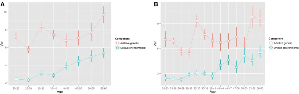
To further verify the periodic pattern of the A component after age 20 years, we performed stratified analyses with 5-year and 3-5-year intervals based on the AE model. The result based on the 5-year interval (Figure 8A) was very close to that from the AE(t) model (i.e., the B-spline model) and the result based on the 3-year interval (Figure 8B) was more similar to that from the AE(t)-p model (i.e., the P-spline model), which showed more periodicfluctuations. Smaller age intervals of-fered a refined picture but resulted in larger estimation uncertainty.

Discussion

In this work, we have proposed two novel twin models to explore dynamic behavior of the variance components over age or time. The estimated variance functions can be utilized

to calculate the age-specific heritability. The results of our BMI study demonstrate that the proposed models provide a more detailed dynamic profile of the A, C, and E variance compo-nents than the classical twin models. These models are more

flexible than the parametric models (Purcell 2002) as they do not require a prespecified assumption of the function form. Compared to LOSEM, which is an exploratory method and the results of which are heavily dependent on the selection of the width of a weighting distribution (Brileyet al.2015), the proposed models based on P-splines are more adaptive to data and straightforward for model comparison using likeli-hood-ratio tests.

The ACE(t)-p model is more stable than the ACE(t) model in the sense that it is less sensitive to the number of knots. This amounts to the problem in stratification analyses, that is, how to choose age intervals. The ACE(t)-p model solves this issue by penalizing the smoothness to select the best model. More-over, the simulation results suggest that the ACE(t)-p model has the advantage of providing better estimates in terms of AMSE; however, the benefit comes from the price of more computational intensity with the same number of knots. It is evident from the simulation study that adding excessive knots in the ACE(t) model worsens the performance for smooth functions. The ACE(t)-p model also performs better with fewer knots provided the number of knots is sufficient but its performance is less affected than that of the ACE(t) model. Thus, assuming that the variance components rarely change drastically within a short period of time, a preferable strategy is to use the ACE(t)-p model and to choose a moderate number of knots [a number of 10 for each component seems enough based on our simulation, although 35-40 is almost adequate for all smooth functions (Ruppert 2002)] to ensure that the model can sufficiently capture the dynamic behavior and in the meantime does not substantially lose performance or in-crease computational intensity.

variance functions requires a relatively large sample size (at least tens of thousands). Given the current implementation using C++ in the ACEt R package, for a study consisting of 10,000 twin pairs, an Intel i5-3210M laptop takes a few seconds for the ACE(t) model, depending on the number of knots, while it takes around two times longer for the ACE(t)-p model under the same setting. The iterative algorithm for the ACE(t)-p model usually converges within 10 steps.

The trend of the A and C components estimated from the Finnish twin data set for BMI before age 20 years is consistent with that in previous reports (Lajunenet al.2009; Silventoinen et al. 2009) except that the estimated variance of the C component before age 15 years is higher than that from the stratified study (Lajunenet al.2009). This is probably caused by the lack of adequate observations at the ages of 13 years and 15 years (Figure 2). It is also possible that the steep de-cline at the beginning is too rapid for the splines with the order of 3 to capture. Given the absence of the C component, our variance curves of the A and E components indicate that the heritability [estimated as s2

aðtÞ=ðs2aðtÞ þs2eðtÞÞ]

de-creases gradually to,50% until age 50 years. This is in ac-cordance with a previous report in which samples were stratified by 10-year age groups (Korkeilaet al.1991) and a meta-analysis of twin studies showing that the heritability of BMI is higher among adolescents than among adults (Elks et al.2012). Our estimated variance curves suggest that the decreasing heritability of BMI during middle age is due to the remarkable growth of the unique environmental variance, highlighting the importance of the environmental role in con-trolling BMI among adults. The variance of the genetic com-ponent stabilizes after age 20 years, possibly caused by the end of the physiologically developmental phase that is infl u-enced substantially by genetic factors. It may also relate to the effect size of the SNP rs9939609 inFTOon BMI that rises until around age 20 years and then gradually attenuates into adulthood (Hardyet al.2010). In contrast, the heritability of 76% from the ACE and AE models is overestimated for age .20 years as our variance curves suggest that the heritability falls below 50% after age 40 years.

Comparing the variance curves from the different models in the Finnish BMI study shows thatfitting data using a wrong model may lead to severely misleading results and interpreta-tion. For instance, ignoring the age-dependent effect on the E component inflated the estimation of the variance of the genetic component. As the heterogeneous genetic or environmental effects of age seem ubiquitous for many complex traits, previous twin studies based on the classical twin models (Distelet al. 2011; Elkset al.2012; Saset al.2012) might produce an in-accurate estimate of heritability. Explicitly modeling the vari-ance functions is a necessary action if we want to know more about their strength. Our proposed models provide unprece-dentedly refined details for the evolution of both genetic and environmental factors, which pave the way to explore the age-specific heritability function. Identification of the dynamic be-havior of the genetic factor likely implies the interaction with age of some key genes related to the phenotype such asFTOfor

BMI. Our results provide support for the need to further in-vestigate time-dependent effects of significantly associated SNPs identified in GWAS. In fact, multiple significant SNPs have been found to affect BMI with different temporal patterns during middle age (Daset al.2011).

Future work of the proposed models can be focused on the extension to other types of traits such as binary and categorical traits. A full Bayesian method may be utilized to obtain a more accurate estimate and C.I.’s. Moreover, the proposed models can also be utilized to investigate other timescales and other moderators shared by a twin pair such as birth year. Similar to LOSEM, a major limitation is that the age has to be measured at the twin level (Brileyet al.2015). Further generalization to the variance–covariance matrices using covariance functions (Pletcher and Geyer 1999) is necessary to extend the models to investigate other continuous environmental moderators that may differ within a twin pair, for example education, incomes, or some physical environmental factors.

In conclusion, we have proposed two novel twin models that estimate dynamic behavior of the variance components in the classical twin models with respect to age. As an alternative and generalization to the classical twin models, we have demon-strated the performance of these models through the simulation and the Finnish BMI studies. Our results have emphasized the importance and implications of these models in facilitating twin studies to investigate the age-specific heritability. Given the evidence of the important influence of age on both genetic and environmental factors, previous studies on heritability estimated from the classical twin models may need further review. It should be noted that in addition to age the proposed models can be used to study other environmental moderators as well, which will remarkably broaden their application.

Acknowledgments

We are grateful to the editors and two anonymous referees for their constructive comments that helped us to sub-stantially improve the presentation of this article. L.H. was

financially supported by the Department of Public Health, University of Helsinki. K.S. was supported by the Academy of Finland (grant 266592). J.K. was supported by the Academy of Finland (grants 265240 and 263278). The research reported in this article was supported, in part, by grants P01 AG043352 and R01AG047310 from the National Institute on Aging. The funders had no role in study design, data collection and analysis, decision to publish, or preparation of the manuscript. The content is solely the responsibility of the authors and does not necessarily represent the official views of the National Institutes of Health.

Literature Cited

Akaike, H., 1969 Fitting autoregressive models for prediction.

Ann. Inst. Stat. Math. 21: 243_–247.

Atchley, W. R., and J. J. Rutledge, 1980 Genetic components of

variability and covariability during ontogeny in the

labora-tory rat. Evolution 34: 1161–1173.

Boker, S., M. Neale, H. Maes, M. Wilde, and M. Spiegel et al.,

2011 OpenMx: an open source extended structural equation

modeling framework. Psychometrika 76: 306–317.

Boomsma, D. I., N. G. Martin, and P. C. Molenaar, 1989 Factor

and simplex models for repeated measures: application to two psychomotor measures of alcohol sensitivity in twins. Behav.

Genet. 19: 79–96.

Booth, J. G., and J. P. Hobert, 1998 Standard errors of prediction

in generalized linear mixed models. J. Am. Stat. Assoc. 93: 262–

272.

Breslow, N. E., and D. G. Clayton, 1993 Approximate inference in

generalized linear mixed models. J. Am. Stat. Assoc. 88: 9–25.

Briley, D. A., K. P. Harden, T. C. Bates, and E. M. Tucker-Drob,

2015 Nonparametric estimates of gene₃environment

inter-action using local structural equation modeling. Behav. Genet.

45: 581_–596.

Byrd, R., P. Lu, J. Nocedal, and C. Zhu, 1995 A limited memory

algorithm for bound constrained optimization. SIAM J. Sci.

Comput. 16: 1190_–1208.

Carlin, B. P., and T. A. Louis, 1997 Bayes and empirical Bayes

methods for data analysis. Stat. Comput. 7: 153–154.

Charmantier, A., C. Perrins, R. H. McCleery, and B. C. Sheldon,

2006 Age-dependent genetic variance in a life-history trait in

the mute swan. Proc. Biol. Sci. 273: 225–232.

Cheverud, J. M., J. J. Rutledge, and W. R. Atchley, 1983

Quantita-tive genetics of development: genetic correlations among

age-specific trait values and the evolution of ontogeny. Evolution

37: 895–905.

Claeskens, G., T. Krivobokova, and J. D. Opsomer, 2009 Asymptotic

properties of penalized spline estimators. Biometrika 96: 529–

544.

Crainiceanu, C., D. Ruppert, and M. P. Wand, 2005 Bayesian

anal-ysis for penalized spline regression using WinBUGS. J. Stat.

Softw. 14: 1–24.

Craven, P., and G. Wahba, 1978 Smoothing noisy data with spline

functions. Numer. Math. 31: 377–403.

Das, K., J. Li, Z. Wang, C. Tong, G. Fu et al., 2011 A dynamic

model for genome-wide association studies. Hum. Genet. 129:

629_–639.

de Boor, C., 1978 A Practical Guide to Splines(Applied

Mathemat-ical Sciences, Vol. 27). Springer-Verlag, New York.

Distel, M. A., J. M. Vink, M. Bartels, C. E. M. van Beijsterveldt, M. C.

Neale et al., 2011 Age moderates non-genetic in_fluences on

the initiation of cannabis use: a twin-sibling study in Dutch

adolescents and young adults. Addiction 106: 1658_–1666.

Efron, B., and R. J. Tibshirani, 1994 An Introduction to the

Boot-strap. CRC Press, Cleveland, OH/Boca Raton, FL.

Eichler, E. E., J. Flint, G. Gibson, A. Kong, S. M. Leal et al.,

2010 Missing heritability and strategies forfinding the

under-lying causes of complex disease. Nat. Rev. Genet. 11: 446–450.

Eilers, P. H. C., and B. D. Marx, 1996 Flexible smoothing with

B-splines and penalties. Stat. Sci. 11: 89–121.

Elks, C. E., M. Den Hoed, J. H. Zhao, S. J. Sharp, N. J. Warehamet al.,

2012 Variability in the heritability of body mass index: a

system-atic review and meta-regression. Front. Endocrinol. 3: 29.

Goeman, J. J., 2010 L1 penalized estimation in the Cox

propor-tional hazards model. Biom. J. 52: 70–84.

Hardy, R., A. K. Wills, A. Wong, C. E. Elks, N. J. Warehamet al.,

2010 Life course variations in the associations between FTO

and MC4R gene variants and body size. Hum. Mol. Genet. 19:

545–552.

Hastings, W. K., 1970 Monte Carlo sampling methods using

Mar-kov chains and their applications. Biometrika 57: 97_–109.

Henderson, C. R., 1975 Best linear unbiased estimation and

pre-diction under a selection model. Biometrics 31: 423_–447.

Kaprio, J., and M. Koskenvuo, 2002 Genetic and environmental

factors in complex diseases: the older Finnish Twin Cohort.

Twin Res. Off. J. Int. Soc. Twin Stud. 5: 358–365.

Kaprio, J., L. Pulkkinen, and R. J. Rose, 2002 Genetic and

environ-mental factors in health-related behaviors: studies on Finnish twins

and twin families. Twin Res. Off. J. Int. Soc. Twin Stud. 5: 366–371.

Kauermann, G., and M. Wegener, 2011 Functional variance

esti-mation using penalized splines with principal component

anal-ysis. Stat. Comput. 21: 159–171.

Kauermann, G., G. Claeskens, and J. D. Opsomer,

2009 Bootstrapping for penalized spline regression. J.

Com-put. Graph. Stat. 18: 126–146.

Korkeila, M., J. Kaprio, A. Rissanen, and M. Koskenvuo,

1991 Effects of gender and age on the heritability of body

mass index. Int. J. Obes. 15: 647_–654.

Krivobokova, T., C. M. Crainiceanu, and G. Kauermann, 2008 Fast

adaptive penalized splines. J. Comput. Graph. Stat. 17: 1_–20.

Lajunen, H.-R., J. Kaprio, A. Keski-Rahkonen, R. J. Rose, L. Pulkkinen

et al., 2009 Genetic and environmental effects on body mass index during adolescence: a prospective study among Finnish

twins. Int. J. Obes. 33: 559_–567.

Li, Z., and M. J. Sillanpää, 2013 A Bayesian nonparametric

ap-proach for mapping dynamic quantitative traits. Genetics 194:

997–1016.

Li, Z., and M. J. Sillanpää, 2015 Dynamic quantitative trait locus

analysis of plant phenomic data. Trends Plant Sci. 20: 822–833.

Li, J., Z. Wang, R. Li, and R. Wu, 2015 Bayesian group Lasso for

nonparametric varying-coefficient models with application to

functional genome-wide association studies. Ann. Appl. Stat.

9: 640–664.

Locke, A. E., B. Kahali, S. I. Berndt, A. E. Justice, T. H. Perset al.,

2015 Genetic studies of body mass index yield new insights for

obesity biology. Nature 518(7538): 197–206.

Manolio, T. A., F. S. Collins, N. J. Cox, D. B. Goldstein, L. A.

Hindorffet al., 2009 Finding the missing heritability of

com-plex diseases. Nature 461: 747–753.

Mao, W., and L. H. Zhao, 2003 Free-knot polynomial splines with

confidence intervals. J. R. Stat. Soc. Ser. B Stat. Methodol. 65:

901–919.

Neale, M., and L. Cardon, 1992 Methodology for Genetic Studies

of Twins and Families. Springer Science & Business Media. Dordrecht, The Netherlands.

Nelson, R. M., M. E. Pettersson, and Ö. Carlborg, 2013 A century

after Fisher: time for a new paradigm in quantitative genetics.

Trends Genet. 29: 669_–676.

Ortega-Alonso, A., K. H. Pietiläinen, K. Silventoinen, S. E. Saarni,

and J. Kaprio, 2012 Genetic and environmental factors infl

u-encing BMI development from adolescence to young adulthood.

Behav. Genet. 42: 73–85.

O’Sullivan, F., 1986 A statistical perspective on ill-posed inverse

problems. Stat. Sci. 1: 502–518.

Pitkäniemi, J., E. Moltchanova, L. Haapala, V. Harjutsalo, J.

Tuomilehtoet al., 2007 Genetic random effects model for

fam-ily data with long-term survivors: analysis of diabetic nephropathy

in type 1 diabetes. Genet. Epidemiol. 31: 697–708.

Pletcher, S. D., and C. J. Geyer, 1999 The genetic analysis of

age-dependent traits: modeling the character process. Genetics 153:

825–835.

Polderman, T. J. C., B. Benyamin, C. A. de Leeuw, P. F. Sullivan, A. van

Bochovenet al., 2015 Meta-analysis of the heritability of human

traits based onfifty years of twin studies. Nat. Genet. 47: 702–709.

Purcell, S., 2002 Variance components models for gene-environment

interaction in twin analysis. Twin Res. Off. J. Int. Soc. Twin Stud. 5:

554–571.

Rabe-Hesketh, S., A. Skrondal, and H. K. Gjessing, 2008 Biometrical

modeling of twin and family data using standard mixed model

Rijsdijk, F. V., and P. C. Sham, 2002 Analytic approaches to twin data

using structural equation models. Brief. Bioinform. 3: 119–133.

Robinson, G. K., 1991 That BLUP is a good thing: the estimation

of random effects. Stat. Sci. 6: 15–32.

Rosenberg, P. S., 1995 Hazard function estimation using

B-splines. Biometrics 51: 874–887.

Ruppert, D., 2002 Selecting the number of knots for penalized

splines. J. Comput. Graph. Stat. 11: 735–757.

Ruppert, D., M. P. Wand, and R. J. Carroll, 2003 Semiparametric

Regression. Cambridge University Press, Cambridge/London/ New York.

Sas, A. A., Y. Jamshidi, D. Zheng, T. Wu, J. Korfet al., 2012 The

age-dependency of genetic and environmental in_fluences on

se-rum cytokine levels: a twin study. Cytokine 60: 108_–113.

Searle, S. R., G. Casella, and C. E. McCulloch, 2009 Variance

Components. John Wiley & Sons, New York/Hoboken, NJ. Silventoinen, K., J. Kaprio, E. Lahelma, and M. Koskenvuo,

2000 Relative effect of genetic and environmental factors on

body height: differences across birth cohorts among Finnish men and women. Am. J. Public Health 90: 627.

Silventoinen, K., and B. Rokholm, J. Kaprio, and T. I. Sørensen,

2009 The genetic and environmental influences on childhood

obesity: a systematic review of twin and adoption studies. Int. J.

Obes. 34: 29–40.

Silventoinen, K., A. Jelenkovic, R. Sund, C. Honda, S. Aaltonen

et al., 2015 The CODATwins Project: the cohort description of collaborative project of development of anthropometrical measures in twins to study macro-environmental variation in genetic and environmental effects on anthropometric traits.

Twin Res. Hum. Genet. Off. J. Int. Soc. Twin Stud. 18: 348–360.

Skrondal, A., and S. Rabe-Hesketh, 2009 Prediction in multilevel

generalized linear models. J. R. Stat. Soc. Ser. A Stat. Soc. 172:

659_–687.

Wood, S. N., 2006 On confidence intervals for generalized

addi-tive models based on penalized regression splines. Aust. N. Z. J.

Stat. 48: 445_–464.

Wu, R., and M. Lin, 2006 Functional mapping - how to map and

study the genetic architecture of dynamic complex traits. Nat.

Rev. Genet. 7: 229_–237.

Yang, J., A. Bakshi, Z. Zhu, G. Hemani, and A. A. E. Vinkhuyzen

et al., 2015 Genetic variance estimation with imputed variants

finds negligible missing heritability for human height and body

mass index. Nat. Genet. 47: 1114_–1120.

Zyphur, M. J., Z. Zhang, A. P. Barsky, and W.-D. Li, 2013 An ACE

in the hole: twin family models for applied behavioral genetics

research. Leadersh. Q. 24: 572_–594.

Appendix

Detailed Derivation of the Estimation in the ACE(t) Model

According to model (1), the estimation ofs2

e;b A_;

andbCis straightforward by minimizing the22 log-likelihood,

ð22Þl¼logjSMj þY9M S2M1YMþlogjSDj þYD9S2D1YD:

The score functions are obtained by calculating the partial derivatives with respect to the parameters,

@ð22Þl

@s2 e

¼trS2_M12YM9S2M1S2 1 M YMþtr

S21 D

2YD9S2D1S2 1 D YD;

@ð22Þl

@bA ¼

BA

TM51231 ₉

diageBATMb A

51231

dS2_D11M_B 21M_BS2_D1YDY9DS2D1

1nM31

þBA

TD51231 ₉

diageBATDb A

51231

dS2_D1A2AS_D21YDY9DS2D1

1nD31;

@ð22Þl

@bC ¼

BC

TM51231 ₉

diageBCTMbC51_231dS21

D 1MB 21MBSD21YDY9DS2D1

1nM31

þBC

TD51231 ₉

diageBCTDbC51_231dS21

D 1DB21DBSD21YDY9DS2D1

1nD31;

wheredðÞis the matrix with only its diagonal elements. The Hessian matrixH_ðbA_;bC_;s2

eÞcan be obtained by further calculating the partial derivatives of the score functions with respect to the parameters. Thus, the MLEscs2

e;bcAk;andbbclcan be obtained by

using numerical methods such as the Newton–Raphson method. Practically, it would be time-consuming because the estima-tion of variance generally requires a relatively large sample size so that the large-scale computaestima-tions for the Hessian matrix would be inevitably involved. Alternatively, we minimize the log-likelihood function without directly calculating the Hessian matrix by using the limited-memory L-BFGS algorithm (Byrdet al.1995) for bound constrained optimization, which is in the family of quasi-Newton methods. In this algorithm, the approximated Hessian matrixH~ is computed in a way that is much faster than the Newton–Raphson method.

Detailed Derivation of the Estimation in the ACE(t)-p Model

We use the difference matrix of the second order (Eilers and Marx 1996) to constructDA¼DTADAandDC¼DTCDC;where

DA ¼ 0

@1 2⋮2 1 ⋯⋱ 0⋮

0 ⋯ 1 22 1

1 A

ðK22Þ3K

and

DC ¼ 0

@ 1 2⋮2 1 ⋯⋱ 0⋮

0 ⋯ 1 22 1

1 A

ðL22Þ3L

:

Given the target function

gbA;bC¼ ð1=2ÞlogjSMj þYM9SM21YMþlogjSDj þY9DS2D1YDþbA9DAbA .

s2

bAþbC9DCbC .

s2 bC

;

@gbA;bC

@bA ¼ 1 2

BA9

TMdiag

eBATMb A

dZ92MS2M1Z2M2Z92MS2M1YMY9MS2M1Z2M

1fM31

þ0:5BA_TD51231 ₉

diageBATDb A

51231

dS2_D12S_D21YDY9DS2D1

1nD31

þBA9

TDdiag

eBATDb A

dZ92DS2D1Z2D2Z92DS2D1YDY9DS2D1Z2D

1fD31þ

DAþD9AbA s2

bA

;

@gbA;bC

@bC ¼ 1 2

BC9

TMdiag

eBCTMbC_dZ9_3MS21

M Z3M2Z93MS2M1YMY9MS2M1Z3M

1fM31

þBC9

TDdiag

eBCTMb C

dZ93DS2D1Z3D2Z93DS2D1YDY9DS2D1Z3D

1fD31þ

DCþD9CbC s2

bC

:

Through straightforward matrix operations, it follows that the second derivative after applying expectation over (YM;YD) by

recalling thatEðY9PYÞ ¼trðPSÞfor a nonstochastic matrixPis

g$ðbA;bCÞ ¼1 2 _{G11 G12} G’ 12 G22 ;

G11¼s22 bAd

DAþD9A

þBA9

TMdiag

e2BATMbA_dZ9_2MS21 M 1MBS2

1 M Z2M

BA

TM

þ0:25BA_TD51231 ₉

diage2BATDbA51_231d S21 D S2

1 D

BA

TD51231

þBA9

TDdiag

e2BATDbA_dZ9_2DS21 D S2

1 D Z2D

þ0:5dZ92DS2D11DBS2 1 D Z2D

BA

TD

G12¼BC9

TMdiag

eBCTMbCþBATMbA_dZ9_3MS21 M 1MBS2

1 M Z3M

BA

TMþ0:5B C9

TDdiag

eBCTDbCþBATDbA_dZ9_3DS21 D S2

1 D Z3D

þZ3D9 S2D11DBS2 1 D Z3D

BA

TD;

G22¼s2 bCd

DCþD9C

þBC9

TMdiag

e2BCTMbC

dZ93MSM11MBSM1Z3M

BC TMþB

C9

TDdiag

e2BCTDbC

dZ93DSD11DBSD1Z3D

BC TD:

To perform the L-BFGS algorithm in step 2, we calculate the score functions givenðbcA_;bcC_Þ;

@ð22Þlpsp

s2

e;s2_bA;s2_bC

@s2 bA

¼2s24 bA

c

bA_9DAbcA_þ K~ s2 bA

þtr g$bcA;bcC2 1@g$

_c

bA_;bcC

@s2 bA 0 B @ 1 C A;

@ð22Þlpsp

s2

e;s2_bA;s2_bC

@s2 bC

¼2s24 bC

_c

bC_9DCbcC_þ ~L s2 bC

þtr g$bcA;bcC21@g$

_c

bA_;bcC

@s2 bC 0 B @ 1 C A;

@ð22Þlpsp

s2

e;s2_bA;s2_bC

@s2 e

¼trS2M1

2Y9MS2M1S2M1YMþtr

S21 D

2Y9DS2D1S2D1YDþtrðg$

c

bA_;bcC21@g$

_c

bA_;bcC

@s2 e

Þ;

where

@g$bcA;bcC

@s2 bA

¼ 20:5s2_bA4

_dð

DAþD9AÞ 0

0 0

;

@g$bcA;bcC

@s2 bC

¼ 20:5s2_bC4

0 0

0 dðDCþD9CÞ

@g$bcA;bcC

@s2 e

¼1 2

@G11

@s2 e

@G12

@s2 e

@G12

@s2 e

9 @_@G22_s2 e 0

B B B @

1 C C C A;

where

@G11

@s2 e

¼2BA9 TMdiag

e2BATMb

A

dZ2M9 S2M1SM211MBS2M1Z2M1Z2M9 S2M11BMS2M1S2M1Z2M

BA TM

20:5BA_TD51231

9diage2BATDbA51₂₃₁

dS2_D1S2_D1S_D21BA_TD51231

2BA9

TDdiag

e2BATDbA

d2Z2D9 SD21S2D1S2D1Z2D 1Z92DS2D1SD211DBS2D1Z2DþZ92DS2D11DBS2D1S2D1Z2D

BA TD;

@G12

@s2 e

¼ 2BC9

TMdiag

eBCTMb C_þBA

TMb A

dZ93M S2M1S2 1 M 1MBS2

1

M Z3M1Z93MS2M11MBS2 1 M S2

1 M Z3M

BA

TM

2BC9

TDdiag

eBCTDbCþBATDbA

dZ93DS2D1SD21S2D1Z3DþZ93DS2D1SD211DBS2D1Z3D

1Z93DS2D11BDS2D1S2D1Z3D

BA TD;

@G22

@s2 e

¼ 2BC9

TMdiag

e2BCTMbC

dZ93MS2M1SM211MBS2M1Z3MþZ93MS2M11BMS2M1S2M1Z3M

BC TM

2BC9

TDdiag

e2BCTDb C

dZ93DS2D1S2 1 D 1DBS2

1

D Z3DþZ93DS2D11DBS2 1 D S2

1 D Z3D

BC

TD:

Construction of the Confidence Intervals in the ACE(t)-p Model

Let us denoteY ¼ ðYM;YDÞandb¼ ðbA;bCÞ:It has been proposed that treating the P-splines under a framework of a random

effects model has the advantages of giving a better estimate of the variance ofb^(Ruppertet al.2003). In our context, givens2 bA ands2

bC;according to the model assumption,gðbÞis the logarithm of the joint distributionfðb; YÞofYandb:However, when we treatbas random effects, a BPbfor the random effects defined as the mean of the posterior distribution given data from the perspective of the Bayesian framework,i.e.,EðbjyÞ;has the following desirable properties (Searleet al.2009),

E

b

¼EyEðbjyÞ¼EðbÞ;

Var

b2b¼EyVarðbjyÞ:

It is, however, not as straightforward to obtainEðbjyÞandEyðVarðbjyÞÞin this case as the BLUP (Henderson 1975) in the linear

mixed model because the posterior distribution ofbis not available in a closed form. Note thate2gðbÞ_{is proportional to the} posterior distribution ofb:Therefore, various numerical methods can be used to approximate the posterior distribution based one2gðbÞ_{;from which the estimated BPb;the prediction errorVarðb2bÞ;and thus the C.I.’s can be derived.}

Here we give a simple Metropolis–Hastings (MH) algorithm (Hastings 1970) to numerically obtain the posterior distribution ofbgivends2

bA andds2_bC;which is proportional to the joint distribution ofYandb;

e2gðbÞ¼exp 21 2

logjSMj þY9MS2M1YMþlogjSDj þY9DS2D1YDþb A9_DAbA

s2 bA

þbC9DCbC s2

bC !

;

described as follows:

1. Set the initial value ofbð1Þat 0.

2. Propose the nextbðiþ1Þby sampling fromN ðbðiÞ;s2

pIÞ:

4. Ifu,e2ðgðbðiþ1Þ_Þ2gðbðiÞ_ÞÞ

;acceptbðiþ1Þ:Then go back to step 2.

The variances2

pof the proposal distribution affects the performance of the MH algorithm in terms of convergence. In our

simulation and real data study, we sets2

p¼0:1 and the trace plots showed the chains mixed quickly. The MCMC samples can

give us accurate estimates ofbandVarðbjyÞunder the guarantee of adequate numerical precision. We found in the simulation study that the posterior mean b is often quite close to the modebb; suggesting that the posterior distribution is highly symmetric. The conditional MSE of prediction VarðbjyÞ is proposed to be a better estimate of prediction error than Varðb_{2bÞ(Skrondal and Rabe-Hesketh 2009), which thus is adopted to compute the C.I.’s in our analyses. Alternatively,}

a parametric bootstrap method can be used to estimateEyðVarðbjyÞÞby generating a set of bootstrap replicatesy* from the

empirical distributionbfðyÞaccording to model (1) with the parameters replaced by their estimates from the EM algorithm. Thus, the variances dVarðBAðtÞbAÞ and Varðd BCðtÞbCÞ at the time t are expressed as BAðtÞ9Varðd bA2bAÞBAðtÞ and BC_{ðtÞ9dVarðb}C_2bC_ÞBC_{ðtÞ;wheredVarðb}A _2bA_Þ

anddVarðbC2bCÞare estimated from the MCMC outputs. It should be pointed out that the estimated variances do not take into account the variability of ds2