INVESTIGATION
Selecting Informative Traits for Multivariate
Quantitative Trait Locus Mapping Helps to Gain
Optimal Power
Riyan Cheng,*,1Justin Borevitz,* and R. W. Doerge†,1 *Division of Plant Sciences, Research School of Biology, The Australian National University, Canberra, Australian Capital Territory 0200, Australia, and†Department of Statistics, Purdue University, West Lafayette, Indiana 47907
ABSTRACTA major consideration in multitrait analysis is which traits should be jointly analyzed. As a common strategy, multitrait analysis is performed either on pairs of traits or on all of traits. To fully exploit the power of multitrait analysis, we propose variable selection to choose a subset of informative traits for multitrait quantitative trait locus (QTL) mapping. The proposed method is very useful for achieving optimal statistical power for QTL identification and for disclosing the most relevant traits. It is also a practical strategy to effectively take advantage of multitrait analysis when the number of traits under consideration is too large, making the usual multivariate analysis of all traits challenging. We study the impact of selection bias and the usage of permutation tests in the context of variable selection and develop a powerful implementation procedure of variable selection for genome scanning. We demonstrate the proposed method and selection procedure in a backcross population, using both simulated and real data. The extension to other experimental mapping populations is straightforward.
I
T is a common practice to collect data on multiple pheno-types when conducting a quantitative trait locus (QTL) mapping experiment. Historically, multiple traits are ana-lyzed separately (referred to as single-trait analysis) (Edwardset al.1987; Stuberet al.1987; Welleret al.1988; Hubner et al.2005). Single-trait analysis does not benefit from additional information that can be gained from the correlations between traits. Therefore, multitrait analysis has been advocated in the QTL mapping community for many years (Jiang and Zeng 1995; Korol et al. 1995, 1998; Ronin et al. 1995; Knott and Haley 2000; Verzilli et al. 2005). By accounting for information in the residual covariance of certain traits, multitrait analysis has the po-tential to achieve a higher statistical power for QTL detec-tion and result in more accurate estimates than single-trait analysis (Jiang and Zeng 1995). Furthermore, multitraitanalysis allows formal studies of biologically interesting hy-potheses such as pleiotropy (Mangin et al.1998) and QTL-by-environment interaction (Piepho 2001).
As one of the main motivations, multitrait analysis is employed to increase statistical power for QTL detection. Unfortunately, it is not always more powerful than single-trait analysis (Jiang and Zeng 1995; Korol et al.1995; Wu et al. 1999). Jiang and Zeng (1995) and Korol et al.(1995) dem-onstrated that the statistical power of multitrait analysis depends on both the QTL effects and the structure of the re-sidual covariance of the traits. Moreover, in situations where the number of traits is large [e.g., expression QTL (eQTL) analysis], it may not be possible to include all the traits in one analysis, using a usual multivariate approach. The shrink-age technique (Tsai and Chen 2009) can resolve the largep, smallnproblem but it is computationally intensive and thus may not be feasible in QTL mapping that typically scans a large number of marker loci. A critical question is, Which traits should be analyzed in the multitrait framework? While Ronin et al. (1998) focused on multitrait analysis of pairs of traits, Knott and Haley (2000) suggested several considerations for multitrait studies that may be difficult to exercise. To address these issues we propose variable selection (Rencher 1993, 1998) as a strategy to choose a subset of traits for multitrait analysis. The proposed approach makes the most of multitrait Copyright © 2013 by the Genetics Society of America
doi: 10.1534/genetics.113.155937
Manuscript received May 13, 2013; accepted for publication August 7, 2013 Available freely online through the author-supported open access option. Supporting information is available online athttp://www.genetics.org/lookup/suppl/ doi:10.1534/genetics.113.155937/-/DC1.
1Corresponding authors: Division of Plant Sciences, Research School of Biology, The Australian National University, Canberra, Australian Capital Territory 0200, Australia. Email: [email protected]; Department of Statistics, Purdue University, 250 N. University St., W. Lafayette, IN 47907. E-mail: [email protected]
analysis in terms of statistical power for QTL detection and is demonstrated for backcross populations, using Hotelling’sT2 statistic (but does not depend on this test statistic), and can be extended to other populations. Since the ultimate goal of QTL mapping is to detect genomic regions that are associated with specific traits or biological processes, the proposed method can provide such information and thus facilitate interpretation of the results.
Materials, Methods, and Results
Real data and preliminary analyses
We considered expression trait (e-trait) data of 211 recombi-nant inbred lines (RILs) that were derived from two parental inbred Arabidopsis thaliana accessions, Bayreuth-0 (Bay-0) and Shahdara (Sha), by selfing (Loudet et al. 2002; Kim 2007; Westet al.2007). Affymetrix technology (Kliebenstein et al. 2006) was employed to generate the microarray data (available in theArrayExpressdatabase with query “E-TABM-126”). Ninety-five distributed markers contributed genotypic information across thefive chromosomes (Westet al.2006). The maximum genetic distance between two adjacent markers was 10.944 cM, the minimum was 2.224 cM, and the median was 4.771 cM (Figure S1 in supporting information,File S1). There are.23,000 genes in the repository. Rather than look-ing at all of them, we focused on the expression transcripts of 16 genes (i.e., 16 e-traits; Table S1 inFile S1), which are in a well-studied defense pathway, from a control environment (Wanget al.2005). Considerations for choosing a small data set include the following: (a) it is computationally easier to establish a methodology using a relatively small data set; (b) our current proposed method is most suitable for small or moderately large data although strategies can be explored to apply it to very large data (section 9 inFile S1); and (c) if we study the whole set, interpretation of results will be of first importance; however, this is beyond the scope of our study. In addition to these 16 e-traits, we also considered thefirst 50 e-traits in the same repository when we assessed the method we proposed later, using simulations.
We first employed a single-trait single-marker approach for analysis of theA. thalianadata. We calculated Hotelling’s T2 test statistic at each of the 95 markers and performed 10,000 permutations of the genotypic data to estimate the 0.05 significance threshold, which was 16.44276, adjusted for all 95 markers and for all 16 e-traits. A marker was de-clared to have a significant association with an e-trait only if theT2value was a local maximum along the genome and was equal to or larger than the estimated threshold. If two markers on the same chromosome had a significant associa-tion with the trait but the test statistic at any marker between them was not smaller than the smaller test statistic at these two markers by two standard deviations of the null distribu-tion that was estimated by the permutadistribu-tion test, then the marker with the smaller test statistic was ignored. This was to prevent adjacent markers from being identified as QTL
purely due to linkage. With these criteria, the single-trait single-marker approach identified 11 markers (At1g11360-4, At1g31580-11, At2g03750-5, At2g14560-2, At2g17240-6, At2g42680-9, At3g61100-9, At5g10380-10, At5g44320-4, At5g45110-11, and At5g48180-4) that were associated with the 16 e-traits at genome-wide significance level 0.05 (Figure 1A; see section 4 inFile S1for more information).
We then considered joint analysis of all 16 e-traits and employed a multitrait single-marker approach for theA. thaliana data. We calculated Hotelling’sT2test statistic at each of the 95 markers and performed 10,000 permutations of the genotypic data to estimate the 0.05 significance threshold, which was 46.33388. With the same criteria as in the single-trait analysis, the multitrait single-marker approach identified 12 markers (At1g11360-4, At1g31580-11, At2g14560-2, At2g17240-6, At2g26640-8, At2g45140-3, At3g10720-6, At3g56360-7, At5g06660-5, At5g24930-6, At5g44320-4, and At5g53940-10) that were associated with the 16 e-traits at genome-wide significance level 0.05 (Figure 1B). Among the identified markers, At2g17240-6, At3g10720-6, At5g24930-6, and At5g44320-4 are at least 10 cM from any of the flanking markers of the 16 e-trait network genes. Two of these 12 markers, At3g10720-6 and At5g24930-6, were not detected when we analyzed the traits separately.
We were interested in taking a closer look at markers 10 (At1g31580-11), 27 (At2g14560-2), 42 (At3g10720-6), and 55 (At3g56360-7). Single-trait analysis disclosed only one trait to associate with marker 10 but many traits with marker 27. The multitrait analysis of the 16 e-traits detected a QTL at marker 42 while single-trait analysis did not show any such evidence. Finally, both single-trait and multitrait analyses detected a QTL at marker 55; however, the single-trait mapping curve at this marker barely crossed the threshold line (Figure 1).
Selecting traits for multitrait analysis
The addition of a trait to a multivariate analysis is not always justified in terms of the statistical power for QTL detection. Generally, unique information about QTL affecting a trait is reduced in the presence of other traits. We can use this knowledge to select informative traits for multitrait QTL analysis. In fact, traits can be chosen such that the selected ones collectively contribute most to the test statistic and attain an optimal power for QTL detection.
Suppose there arep traits (y1,y2,. . .,yp). LetLy1;y2;⋯;yk be Wilks’L, a test statistic commonly used in multivariate hypothesis testing, corresponding to (y1, y2,. . .,yk) and Lykþ1jy1;y2;:::;yk¼Ly1;y2;:::;ykþ1 = Ly1;y2;:::;yk, 0#k,p. Rencher (1993) shows that
Fykþ1jy1;y2;:::;yk¼ 12Ly
kþ1jy1;y2;:::;yk Lykþ1jy1;y2;:::;yk
VE2k
VH (1)
is distributed as Fd:f:H;d:f:E2k, where d.f.H and d.f.E are degrees of freedom for hypothesis and error, respectively. In a backcross or recombinant inbred lines where there are
two possible genotypes, Hotelling’sT2-test statistic can take the place of Wilks’L, and
Fykþ1jy1;y2;:::;yk¼ ðn2k22ÞT 2
y1;y2;:::;ykþ12T 2
y1;y2;:::;yk T2
y1;y2;:::;ykþn22
: (2)
ðT2
∅¼0Þ is distributed asF1,n2k22, whereTy21;y2;:::;yk is Hotel-ling’s statistic based on (y1,y2,. . .,yk) andnis the sample size.
The statistic Fykþ1jy1;y2;:::;yk may be used to test whether a trait is redundant in the presence of other traits and to select traits for multitrait analysis. If there is a predefined order in which the traits are tested for association with a marker, the traits can be tested one by one in that order. If, however, there is no such predefined order, a subset of the traits that collectively contribute most to the test statistic (e.g., Hotelling’sT2) can be selected for QTL mapping. In this
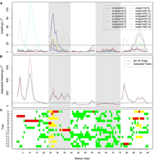
Figure 1 (A–C) Mapping profiles for single-trait analysis of the 16 traits (A) and multitrait analysis of selected traitsvs.that of all 16 traits (B) and selected traits (C). The horizontal lines are 0.05 significance thresholds adjusted for all the markers (and all the traits in the case of single-trait analysis). Each vertical section displays one chromosome. C shows if a trait is selected for multitrait analysis (green), if the single-trait mapping curve goes above the threshold line at the locus (yellow), and if both occur (red).
situation, (1) or (2) does not have the expectedF distribu-tion because of selecdistribu-tion bias, and therefore we cannot rely on F tests to select traits. Instead, model selection techni-ques such as stepwise procedures can be employed (Rencher 1998). An entry/stay value can be specified to determine whether a trait should be selected. Alternatively, as demon-strated later we can select a given number of traits that contribute most to the test statistic. Multitrait analysis can be performed on the resulting subset of the traits to test for the association between the marker and the traits.
In the case of two traits, Cheng (2007) showed that if a QTL has an effect on trait 1 but no effect on trait 2, then the contribution of trait 2 to Hotelling’sT2given trait 1 tends to infinity as the residual correlation between the two traits goes to 1 (or21). In general, we have the following prop-osition (see section 1 inFile S1for more information).
Proposition 1.If a QTL has a nonzero effect on one trait but no effect on another trait,then the power to detect the QTL goes to 100%as the residual correlation between the two traits goes to1 (or21).
As we will see later, Proposition 1 is very useful for multitrait analysis. In many situations, we may expect a QTL to have no effect, or a relatively negligible effect, on some trait (trait 2) but an intermediate effect on another trait (trait 1). We may not have sufficient power to detect this QTL with single-trait analysis. However, joint analysis of these two traits will have an increase in power to detect it if these two traits are closely correlated. This conclusion is not limited to the case of two traits (see section 9 inFile S1for examples).
Impact of selection bias on type I error rates and statistical power
Selection bias can invalidate significance thresholds that are based on the expected F distribution of (1) or (2) and result in inflated type I error rates even in simple situations where a single marker is tested for QTL. It may be possible to empirically estimate the null distribution of the test statistic, using the permutation test (Churchill and Doerge 1994). There are typically two ways to perform the permutation test: (1) permute the phenotypic data and keep the genotypic data and (2) keep the phenotypic data and permute the genotypic data. We chose the latter here since permuting genotypic data allows the relationship between the trait and covariates (if any) to be retained, which may result in better estimation (O’Gorman 2005; Cheng and Palmer 2013). However, how to actually perform the permutation test in variable selection is not obvious. There are many ways to select traits from the permuted data to estimate significance thresholds. In this study, we investigated four intuitive methods: (A) use the same“best”traits as selected from the original data (i.e., data without permutation), (B) select the same number of best traits as selected from the original data, (C) use the same procedure as selecting best traits from the original data, and (D) select a predefined number of best traits if this num-ber is predefined to select best traits from the original data.
We assumed that in methods A, B, and C the number of traits selected from the original data was not predefined and an entry/stay value was specified for a model selection proce-dure to select an optimal subset of traits.
Type I error rate:Wefirst investigated the capability of the above four methods to control type I error rates. We em-ployed 1000 simulations to estimate type I error rates. In each simulation, we simulated 16 traits from a multivariate normal distribution whose mean and variance–covariance were re-spectively equal to the sample mean and variance–covariance, after adjusting for QTL effects at marker 42 (At3g10720-6), of the actual 16Arabidopsis thalianae-traits as detailed pre-viously, and used the real genotypic data at marker 42. This marker was among the markers of interest since at this marker multitrait analysis of all 16 traits identified a QTL but single-trait analysis did not (Figure 1). We performed the stepwise backward elimination procedure to select traits. For methods A–C, the entry/stay value (if needed) was 3.886 (= F0.05;1,21122), and if the resulting subset of traits was empty, we selected the trait with the largestT2. For method D, the predefined number of selected traits was 5. We then performed multitrait analysis of the selected traits (we used single-trait analysis and multitrait analysis interchangeably when there was only one trait of interest).
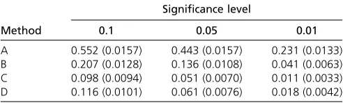
In each of the simulations, we permuted the genotype data 10 times (as in Cheng and Palmer 2013), which resulted in a total of 10,000 permuted data sets, and then applied the four methods to each of the permuted data sets. The thresh-olds were estimated from these 10,000 permutations for each of these methods. A QTL was claimed if the test statistic exceeded the significance threshold estimated by using each of the four methods at a specified significance level. Table 1 displays the estimated type I error rates and their standard errors. We can see that using the same procedure (methods C and D) for the permuted data as in the analysis of the original data controlled type I error rates at the nominal significance levels, whereas using the same traits (method A) or selecting the same number of traits (method B) as selected from the original data resulted in inflated type I error rates.
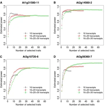
Statistical power and the number of selected traits: The above simulation study indicates that we can employ either method C or method D to get a valid significance threshold if variable selection is performed to select traits for multitrait analysis. For method C, the number of selected traits generally depends on both the data and the entry/stay value. In other words, it will differ for either a different entry/stay value or a different data sample. For method D, one question of interest is that given the total number of traits, how the number of selected traits influences the statistical power, and another question is that given the number of selected traits, how the total number of available traits influences the statistical power. To answer these questions, we considered different sets of traits: (1) the 16 e-traits described and analyzed previously, (2) the 16 e-traits plus thefirst 20 of the additional 50 e-traits
mentioned previously, and (3) the 16 e-traits plus all the additional 50 e-traits. We did not directly use these traits. Instead, we simulated traits by taking advantage of the covariance structure as well its relationship with the QTL effects. Specifically, we simulated traits that followed a mul-tivariate normal distribution with mean being equal to one-fifth, one-third, one-half, or one-half of the QTL effects estimated from these traits at markers 10 (At1g31580-11), 27 (At2g14560-2), 42 (At3g10720-6), or 55 (At3g56360-7) and variance–covariance being equal to the residual variance– covariance estimated from those traits at the marker. Specify-ing a good covariance structure and QTL effects for simulations is not always easy. Fortunately, the covariance structure and the putative QTL effects at the markers were available, so we took advantage of this information by adjusting the QTL effects to observe a visually improved pattern in the power so that the estimated power was not too large or small to disguise impor-tantfindings. We simulated 1000 data sets. In the analysis of each data set we selected the best subsets of all possible num-bers of traits and then estimated the significance thresholds, using 5000 permutations of the genotypic data. Figure 2 shows the estimated power at significance level 0.05 for different numbers of selected traits from all 3 sets of available traits. We can see that the statistical power tended to increase as the number of selected traits increased, and the gain in power was large at the beginning but quickly decreased and became negligible at some point. There were cases where the power attained or approximated the maximum with less than one-third of the traits and a larger number of selected traits resulted in a lower power. For a relatively small number of selected traits, the statistical power was lower if the total number of traits was larger, meaning a more serious selection bias.
A variable selection procedure
As shown previously, we could employ method C or D to appropriately determine the decision rule via the permutation test. For method C, we needed to predefine an entry/stay value; however, what could be such a good value for optimal power was in question and choice of a good entry/stay value would be complicated by noting that such a value should vary with the total number of traits and likely be any number in a region on the real line. Alternatively, we could use method D and select a number of traits such that any additional trait
contributes little to the statistical power according to a certain criterion. In this spirit, we proposed the following procedure to choose an optimal number of traits at a marker locus [referred to as variable selection for the optimal power procedure (VSFOP)]:
1. Determine the maximum number, K, of traits to be selected.
2. Take 1000 (say) nonparametric bootstrap samples and estimate the statistical power as well as its standard error for k = 1, 2,. . .,K best traits, denoted by pk and ek, respectively.
3. Choose the largest k*(#K) such thatpk*$pk*þ12ek*þ1 andpk*21,pk*2ek*.
The maximum number K should be much smaller than the sample size to ensure the parameters are estimable and the variation of the estimates is not overly large. In practice, it may be most useful to identify a handful of traits for an extended study and therefore, in addition to saving unnec-essary computational cost, the maximum numberKshould not be too large to facilitate biological interpretation of the findings. In our data, we simply usedK= 16. To take ad-vantage of multitrait analysis, we chosek* = 2 ifk*#1. The above procedure dynamically determines the optimal number of traits at a marker. Since the number of selected traits can vary across different markers, the test statistics may not be comparable. For easy comparison across scan-ning loci, we proceeded with another step:
4. Scale the test statistic at locusi(i= 1, 2,. . .,L),T(i), by v=vito get a new statisticT~ðiÞ; that is,T~ðiÞ ¼TðiÞ3v=vi, where v . 0 and vi is the estimated threshold for locus i at a given genome-wide significance level asuch that P(|T(i)| ,vi, i = 1, 2,. . .,L) $1 2 a. We may impose the condition P(|T(1)| , v1), P(|T(2)|,v2) =. . .=P(|T(L)|,vL).
We applied the above procedure to the e-trait data. The selected traits at each marker are displayed in Figure 1C (see Figure 3A for the number of selected traits at each marker) and the mapping result of multitrait analysis of the selected traits is shown in Figure 1B, wherevin the adjusted Hotel-ling’sT2at locusi(i= 1, 2,. . ., 95),T~ðiÞ, was the estimated threshold for multitrait analysis of all 16 traits at genome-wide significance level 0.05. We can see that while the num-ber of selected traits was mostly between 4 and 8, we needed only 2 traits at a large number of markers for the purpose of QTL detection. The mapping profile of selected traits was very similar to that of all traits (Figure 1B), sug-gesting the success of the selection procedure (see section 10 inFile S1for the results of analyzing all 66 e-traits that we considered in the simulations).
It is worth noting that the proposed procedure selected only 2 traits to disclose potential QTL if there was a strong association between a marker and a trait (e.g., marker 3 and trait 3) but selected many more traits if the association be-tween a marker (e.g., marker 42) and any trait was weak. Table 1 Estimated type I error rates and standard errors
Significance level
Method 0.1 0.05 0.01
A 0.552 (0.0157) 0.443 (0.0157) 0.231 (0.0133) B 0.207 (0.0128) 0.136 (0.0108) 0.041 (0.0063) C 0.098 (0.0094) 0.051 (0.0070) 0.011 (0.0033) D 0.116 (0.0101) 0.061 (0.0076) 0.018 (0.0042) Four methods were implemented to select an optimal subset of traits for multitrait analysis of the permuted data: (A) use the same traits as selected in the analysis of the original data, (B) select the same number of traits as in the analysis of the original data, (C) use the same procedure as selecting traits in the analysis of the original data, and (D) select a predefined number (five) of traits. Standard errors of the estimated type I error rates are given in parentheses.
We were interested to explore more at marker 3 about the power of multitrait analysis and the proposed procedure. Variable selection would disclose traits 2, 3, and 12 to be as-sociated with marker 3 (Table S4 inFile S1). However, single-trait analysis did not provide any such evidence for single-trait 2 or trait 12 (Figure 1A). Actually at marker 3, the estimated QTL effects were negligible on trait 16 but intermediate on traits 2 and 12 (section 6 inFile S1). While the opposite effects on and the large correlation between traits 2 and 12 helped to disclose trait 12, the high correlation between traits 2 and 16 led to the disclosure of trait 2. The advantage of multitrait analysis at marker 3 came from the favorable configuration of the QTL effects and the residual correlation structure (see section 6 in
File S1for more examples).
Comparison with clustering and principal components:
Multitrait analysis takes advantage of correlations among traits, which may provide a higher statistical power or more accurate estimation of parameters including QTL location (Jiang and Zeng 1995). However, multitrait analysis may not be feasible under the framework of traditional multivar-iate analysis when the number of traits is large. In such a situation, one may cluster traits and analyze the clustered traits, using a multitrait approach (Chun and Keles 2009).
Alternatively, one can consider principal component analy-sis, which has been proposed for QTL mapping (Welleret al. 1996). We looked at these strategies, using the e-trait data we analyzed above. Recall the data contained 16 e-traits and 95 markers for 211 individuals. We took 500 random subsamples of size 106 (i.e., 50% of the total 211 individuals) from the e-trait data and then analyzed each subsample as follows:
1. We analyzed the traits separately (ST).
2. We determined the number of traits by the proposed VSFOP procedure, using 1000 nonparametric bootstrap samples of the subsample at a marker, and selected that number of traits at the marker, and then analyzed the selected trait using the multitrait approach (SL). 3. We implemented multitrait analysis of all 16 traits (AT). 4. We analyzed clustered traits separately (CL), with clus-ters being defined by hierarchical clustering based on the correlations between the e-traits and by a cutoff of 0.75 (section 7 inFile S1). We did not reestimate the correla-tions using the subsample since the estimation using the total data tends to be more reliable.
5. We analyzed thefirst eight principal components (PC) of the trait data separately (section 8 inFile S1). Suppose the traits in the data wereY, andK was a matrix that chose the subsample; i.e., the traits in the subsample Figure 2 (A–D) Statistical power esti-mated from 1000 replicate simulations at the significance level 0.05
were in the formKY, andVtransformedYto its principal components viaYV. Then the PC traits in the subsample wereKYV. In other words, we relied on the covariance matrix estimated from the total data to calculate the principal component scores.
We estimated 0.05 significance thresholds using method D, adjusted for multiplicity of the tests, using 1000 permu-tations of the genotypic data in the subsample (see section 5 in File S1 for more information). For each of the above
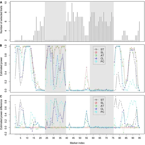
approaches, a marker was defined as a positive if Hotelling’s test statistic,T2, exceeded the 0.05 threshold. Then, a positive should be almost surely due to true QTL or linkage to QTL if the estimated power was apparently .0.05. Figure 3B dis-plays the proportion of the 500 subsamples where each marker was detected as a QTL. The difference in the esti-mated power between the proposed method and any other method is displayed in Figure 3C. Overall, our proposed method had a performance virtually the same as joint analysis Figure 3 (A–C) Number of selected traits (A), estimated statistical power using random 50% subsamples (B), and difference in the estimated power between the proposed VSFOP procedure and any of other methods (C). Five methods were considered: (1) single-trait analysis (ST), (2) multitrait analysis of selected traits (SL), (3) multitrait analysis of all traits (AT), (4) multitrait analysis of clustered traits (CL), and (5) single-trait analysis of thefirst eight principal components (PC). Each vertical section displays one chromosome.
of the 16 traits at most loci and appreciably better in several genomic regions and was more powerful than the remaining three approaches. The proposed procedure dynamically de-termines the number of best traits based on data and preesti-mated power so that it can make the most of power. Note that our method was the most advantageous at loci where a small number of traits were selected (Figure 3); typically, one trait with large QTL effects and one with negligible QTL effects were among the selected traits at those loci, and the trait with negligible QTL effects was just to help in identification of the one with large QTL effects. Multiple-trait analysis of the clus-tered traits tended to work better than single-trait analysis of the principal component variables but seemed to be a compro-mise between single-trait analysis and multitrait analysis of all 16 traits.
Discussion
In this study, we devised a strategy to perform multitrait analysis. Instead of jointly analyzing all available traits, we proposed to select a subset of informative traits and analyze the selected traits by a multitrait approach. Using simulations and real data, we showed our proposed method has the potential to achieve optimal statistical power. To our knowl-edge, this is the first time that variable selection has been proposed for multitrait QTL mapping. We expect our proposed method will have practical applications. For instance, we are usually interested in genetic variants underlying economically important traits such as yield, protein content, quality attrib-utes, and disease resistance in a breeding program. These traits tend to be correlated, and multitrait analysis is preferable to single-trait analysis, as examplified by Singhet al.(2012), who recently studied several wheat diseases. Then, our ap-proach is not only able to attain an optimal power in the framework of multitrait analysis but also able to best disclose traits that are relevant to identified QTL, which may not be desirably delivered by either single-trait analysis or full joint analysis (see section 9 inFile S1for more information).
There are a number of situations where our proposed method can be useful. First, when the number of traits is larger than the sample size (e.g., expression data of thou-sands of available genes), a subset of traits has to be selected if multitrait analysis is implemented without parameter reg-ularization since including all the traits is not feasible due to the limited degrees of freedom. Shrinkage can get around the largep, smallnproblem; however, the computation can be a serious problem in the framework of multivariate anal-ysis where matrix manipulation such as inversion, in addi-tion to choice of a regularizaaddi-tion parameter, is typically involved. Strategies of best applying the proposed method to large amounts of data remain an interesting research topic (section 9 in File S1). Second, the proposed method is also applicable to data where the number of traits is large and we are interested in a small subset of the most relevant traits. For example, in gene expression data we may be in-terested to know which genes are most influenced by an
eQTL (if any). While multitrait analysis typically identifies QTL associated with a group of traits without readily dis-closing which traits are associated with the QTL, variable selection chooses traits that are statistically most significant and thus most likely involved in a biological process (section 9 inFile S1). Third, information from variable selection can also be useful when we test other biological hypotheses such as pleiotropy. Suppose a trait is not selected (multiple rounds of selection may be required; see section 9 inFile S1
for more information); then the QTL is negligible or of no effect. We do not need to look at pleiotropy if either of two traits is not selected, and we can proceed to test pleiotropy without difficulty if both of two traits are selected.
Variable selection is a data reduction technique. We com-pared our proposed method to another data reduction ap-proach, namely, principal component analysis (Weller et al. 1996), and showed with real data that our method outper-formed it in terms of statistical power. There are other disad-vantages of principal component analysis. First, it is not obvious which traits are associated with the detected QTL. Second, there is a question of how many principal components are to be analyzed. In the e-trait data, it seemed appropriate to an-alyze thefirst four principal component variables but the sev-enth and eighth, which accounted for tiny proportions of the total variance, were among those that identified QTL (Figure S4 and Figure S5 inFile S1). The statistical power would tend to be much lower at most loci if we looked only at the first four principal component variables (data not shown).
One may attempt to cluster the traits based on correla-tions and then analyze the clustered traits via multitrait analysis. Since the power of multitrait analysis depends on both the QTL effects and the correlation structure, it is not possible for analysis of clustered traits to work best at loci of different QTL effects. In contrast, variable selection dynam-ically selects traits according to QTL effects and correlations among traits and multitrait analysis of selected traits mostly works well, and our proposed selection procedure can fully exploit data to provide the best power. Moreover, how to cluster traits and to determine the number of clusters will have an impact on results. In terms of statistical power for the e-trait data, analysis of clustered traits seemed to be somewhere between single-trait analysis and multitrait analysis of all the traits (Figure 3 and section 7 ofFile S1). We introduced the variable selection approach using sta-tistic (1) but we do not have to rely on it to perform variable selection. The model-based maximum-likelihood ratio statistic is more flexible and allows inclusion of identified QTL as covariates in variable selection without any problem. Then we may identify multiple QTL one after another as in single-trait multiple-QTL mapping. However, since variable selection can associate different traits with different QTL, a question may be how to best include identified QTL as covariates. Other ques-tions include how to determine suitable cutoffs to claim QTL, especially when the number of traits under consideration varies. Finally, it will also be useful to extend our proposed method to incorporate practical considerations such as
genotype-by-environment interaction and polygenic varia-tion (Singhet al.2012).
Acknowledgments
Two anonymous reviewers and Christina Kendziorski pro-vided helpful comments.
Literature Cited
Cheng, R., 2007 Statistical methods for mapping multiple com-plex traits. Ph.D. Thesis, Purdue University, West Lafayette, IN. Cheng, R., and A. A. Palmer, 2013 A simulation study of permuta-tion, bootstrap, and gene dropping for assessing statistical signifi -cance in the case of unequal relatedness. Genetics 193: 1015–1018. Chun, H., and S. Keles, 2009 Expression quantitative trait loci mapping with multivariate sparse partial least squares regres-sion. Genetics 182: 79–90.
Churchill, G. A., and R. W. Doerge, 1994 Empirical threshold values for quantitative trait mapping. Genetics 138: 963–971. Edwards, M. D., C. W. Stuber, and J. F. Wendel, 1987
Molecular-marker-facilitated investigations of quantitative-trait loci in maize. I. Numbers, genomic distribution and types of gene ac-tion. Genetics 116: 113–125.
Hubner, N., C. A. Wallace, and H. Zimdahl, E. Petretto, H. Schulzet al., 2005 Integrated transcriptional profiling and link-age analysis for identification of genes underlying disease. Nat. Genet. 37: 243–253.
Jiang, C.-J., and Z.-B. Zeng, 1995 Multiple trait analysis of genetic mapping for quantitative trait loci. Genetics 140: 1111–1127. Kim, K., 2007 Statistical issues in mapping genetic determinants
for expression level polymorphisms. Ph.D. Thesis, Purdue Uni-versity, West Lafayette, IN.
Kliebenstein, D., M. West, H. van Leeuwen, K. Kim, R. Doergeet al., 2006 Genomic survey of gene expression diversity in Arabi-dopsis thaliana. Genetics 172: 1179–1189.
Knott, S. A., and C. S. Haley, 2000 Multitrait least squares for quantitative trait loci detection. Genetics 156: 899–911. Korol, A. B., Y. I. Ronin, and V. M. Kirzhner, 1995 Interval
map-ping of quantitative trait loci employing correlated trait com-plexes. Genetics 140: 1137–1147.
Korol, A. B., Y. I. Ronin, E. Nevo, and P. M. Hayes, 1998 Multi-interval mapping of correlated trait complexes. Heredity 80: 273–284. Loudet, O., S. Chaillou, C. Camilleri, D. Bouchez, and F.
Daniel-Vedele, 2002 Bay-0 x shahdara recombinant inbred line pop-ulation: a powerful tool for the genetic dissection of complex traits in arabidopsis. Theor. Appl. Genet. 104: 1173–1184. Mangin, B., P. Thoquet, and N. Grimsley, 1998 Pleiotropic QTL
analysis. Biometrics 54: 88–99.
O’Gorman, T. W., 2005 The performance of randomization tests that use permutations of independent variables. Comm. Stat. Simul. Comput. 34: 895–908.
Piepho, H. P., 2001 A quick method for computing approximate thresh-olds for quantitative trait loci detection. Genetics 157: 425–432. Rencher, A. C., 1993 The contribution of individual variables to
Hotelling’st2, Wilks’sl, andr2. Biometrics 49: 479–489. Rencher, A. C., 1998 Multivariate Statistical Inference and
Applica-tions. John Wiley & Sons, New York.
Ronin, Y. I., V. M. Kirzhner, and A. B. Korol, 1995 Linkage between loci of quantitative traits and marker loci: multi-trait analysis with single marker. Theor. Appl. Genet. 90: 776–786.
Ronin, Y. I., A. B. Korol, and J. I. Weller, 1998 Seletive genotyping to detect quantitative trait loci affecting multiple traits: interval mapping analysis. Theor. Appl. Genet. 97: 1169–1178. Stuber, C. W., M. D. Edwards, and J. F. Wendel, 1987 Molecular
marker-facilitated investigations of quantitative trait loci in maize. II. factors influenceing yield and its component traits. Crop Sci. 27: 639–648.
Singh, , S., M. V. Hernandez, J. Crossa, P. K. Singh, N. S. Bains,
et al., 2012 Multi-trait and multi-environment QTL analyses for resistance to wheat diseases. PLoS ONE 7: e38008. Tsai, C. A., and J. J. Chen, 2009 Multivariate analysis of variance
test for gene set analysis. Bioinformatics 25: 897–903. Verzilli, C. J., N. Stallard, and J. C. Whittaker, 2005 Bayesian
modelling of multivariate quantitative traits using seemingly unrelated regressions. Genet. Epidemiol. 28: 313–325.
Wang, D., N. D. Weaver, M. Kesarwani, and X. Dong,
2005 Induction of protein secretory pathway is required for systemic acquired resistance. Science 308: 1036–1040. Weller, J. I., M. Soller, and T. Brody, 1988 Linkage analysis of
quantitative traits in an interspecific cross of tomato ( Lycopersi-con esculentum 3 Lycopersicon pimpinellifolium) by means of genetic markers. Genetics 118: 329–339.
Weller, J. I., G. R. Wiggans, P. M. VanRaden, and M. Ron, 1996 Application of a canonical transformation to detection of quantitative trait loci with the aid of genetic markers in a multi-trait experiment. Theor. Appl. Genet. 92: 998–1002. West, M. A., and H. van Leeuwen, A. Kozik, D. J. Kliebenstein, R. W.
Doergeet al., 2006 High-density haplotyping with microarray-based expression and single feature polymorphism markers in Arabidopsis. Genome Res. 16: 787–795.
West, M. A. L., K. Kim, D. J. Kliebenstein, H. Leeuwen, R. W. Michelmore et al., 2007 Global eQTL mapping reveals the complex genetic architecture of transcript-level variation in Ara-bidopsis. Genetics 175: 1441–1450.
Wu, W. R., W. M. Li, D. Z. Tang, H. R. Lu, and A. J. Worland, 1999 Time-related mapping of quantitative trait loci underly-ing tiller number in rice. Genetics 151: 297–303.
Communicating editor: C. Kendziorski
GENETICS
Supporting Information
http://www.genetics.org/lookup/suppl/doi:10.1534/genetics.113.155937/-/DC1
Selecting Informative Traits for Multivariate
Quantitative Trait Locus Mapping Helps to Gain
Optimal Power
Riyan Cheng, Justin Borevitz, and R. W. Doerge
File S1
Supplemental Material:
Selec ng Informa ve Traits for Mul variate Quan ta ve Trait Locus Mapping Helps to Gain Op mal Power
1 Condi onal Contribu on of a Trait
For simplicity we provide analy cal jus fica on for proposi on 1 (see the main text) in the case of two genotypes with allelesAand
aat a locus,AAandAain a backcross (orAAandaain a recombinant inbred line). This is based on two considera ons. First, we
can use the well known Hotelling'sT2test sta s c when there are only two genotypes. Second, we can make inference by comparing
pairwise genotypes when there are more than two genotypes at a locus1.
Consider contribu on of traitzto a test sta s c givenptraitsyyy. Writewww= (yyy, z)and denote itsj-th value bywwwj,1orwwwj,2for
AAorAa. The test for QTL can be based on the Hotelling'sT2-test sta s c
Twww2 = ( ¯www1−www¯2)
[ ( 1
n1
+ 1 n2
)SSS ]−1
( ¯www1−www¯2)T (1)
wheren1andn2are the sample sizes forAAandAarespec vely,www¯1= n1
1 ∑n1
j=1wwwj,1
def
= (¯yyy1,z¯1),www¯2=n1
2 ∑n2
j=1wwwj,2
def
= (¯yyy2,z¯2)
and
S S
S =
∑n1
j=1(wwwj,1−www¯1)
T(www
j,1−www¯1) +
∑n2
j=1(wwwj,2−www¯2)
T(www
j,2−www¯2)
n1+n2−2
def
=
SSSyyyyyy SSSyyyz SSSzyyy s2z
With some mathema cal manipula on, (1) turns out to be (R , 1993)
Tyyy,z2 = T
2
y y y +
n1n2
n1+n2
[ˆβββ(¯yyy1−yy¯y2)T−(¯z
1−z¯2)]2
s2
z(1−R2)
= Tyyy2+
(ˆtz−tz)2
1−R2 (2)
whereT2
yyy is Hotelling'sT2 based onyyy,R2 = S S
SzyyySSSyyyyyy−1SSSyyyz
s2
z is the coefficient of mul ple (or simple ifp = 1) determina on ofz regressed onyyyandβββˆ =SSSzyyySSSyyyy−yy1is the vector of the regression coefficients without intercept, andtˆz =
ˆ
β ββ(¯yyy1−¯yyy2)T
sz √
(n1+n2)/n1n2 ,tz =
¯
z1−z¯2
sz √
(n1+n2)/n1n2 .
Equa on (2) sheds light on the contribu on of an addi onal trait to the test sta s cT2in the presence of other traits. Although
addi on of a trait always increases the test sta s c, the cri cal value also increases with the number of traits. Therefore, the increase
inT2may not be sufficient to jus fy the addi on of a par cular trait. As a simple example, considerp= 1with (2) becoming
Ty,z2 =T
2
y+
(Rty−tz)2
1−R2 . (3)
For simplicity, we assume a QTL is located exactly at a marker, and letay= ¯y1−y¯2represent the QTL effect on traity,az= ¯z1−¯z2
represent the QTL effect on traitz. Without loss of generality, assume|ty| ≥ |tz|. From (3), the condi onal contribu on of traitzwill
depend on the magnitudes of bothRty−tzandR. WhenRty=tz, adding traitzfails to increase the test sta s cTy,z2 . Favorable
1Alterna vely, we can use Wilks'Λwhen there are more than two genotypes at a locus.
situa ons include two well known ones: 1) two traits are posi vely correlated and the QTL has a posi ve effect on one trait but a
nega ve effect on the other; 2) two traits are nega vely correlated and the QTL has posi ve or nega ve effects on both traits.
As a prac cal situa on, consider a QTL with a non-zero effect on traityand no effect on traitz(i.e.,tz = 0buttˆz ̸= 0). Then
Ty,z2 = 1+R
2
1−R2T
2
y(≥Ty2; note thatTy2 =t2y) can be arbitrarily large as long asR2is sufficiently large. Therefore, addi on of a trait to
another trait that has an associa on with a QTL can increase the power of detec ng the QTL if the added trait is not associated with
the QTL but is highly correlated with the other trait. Since (3) is con nuous intz, this conclusion applies if the QTL has a negligible QTL
effect on the added trait. A similar statement can be made from (2) forp >1.
2 The Sixteen Genes
Table S1 lists the sixteen genes whose expression transcripts are described and analyzed in this ar cle. We refer to, say, the first trait
as trait 1 or T1 when there is no confusion.
Table S1Sixteen genes, their le flanking markers, and their gene products
Trait Gene Name Le Markera Gene Productb
T1 At1g08450 At1g05385-3 calre culin 3 (CRT3)
T2 At1g09210 At1g05385-3 calre culin 2 (CRT2)
T3 At1g10730 At1g05385-3 clathrin adaptor complexes medium subunit fam-ily protein
T4 At1g30900 At1g30380-6 vacuolar sor ng receptor, puta ve T5 At1g32210 At1g31580-11 defender against cell death 1 (DAD1) T6 At2g01720 At2g01290-10 ribophorin I family protein
T7 At2g34250 At2g30260-4 protein transport protein sec61, puta ve
T8 At2g45070 At2g42680-9 sec61beta family protein
T9 At2g45770 At2g45140-3 signal recogni on par cle receptor protein,
chloroplast (FTSY)
T10 At2g47320 At2g45140-3 pep dyl-prolyl cis-trans isomerase cyclophilin-type family protein
T11 At2g47470 At2g45140-3 thioredoxin family protein T12 At3g54960 At3g52840-4 thioredoxin family protein
T13 At4g22670 At4g21750-2 tetratricopep de repeat (TPR)-containing protein T14 At4g24190 At4g21750-2 shepherd protein (SHD) / clavata forma on
pro-tein, puta ve
T15 At5g07340 At5g06660-5 calnexin, puta ve
T16 At5g61790 At5g57460-7 calnexin 1 (CNX1)
aLe marker is the le flanking marker of the e-trait gene.
bThe informa on was taken from the TIGRArabidopsis thalianaGenome Annota on Database.
3 Gene c Map
Figure S1 is a gene c map of the 95 gene c markers that are described and used in this ar cle.
Figure S1Gene c map for theArabidopsis thalianadata. Ninety five markers are densely distributed across five chromo-somes. The marked intervals contain one or more of the 16 e-trait network genes.
4 More on Single-trait Analysis of the E-Trait Data
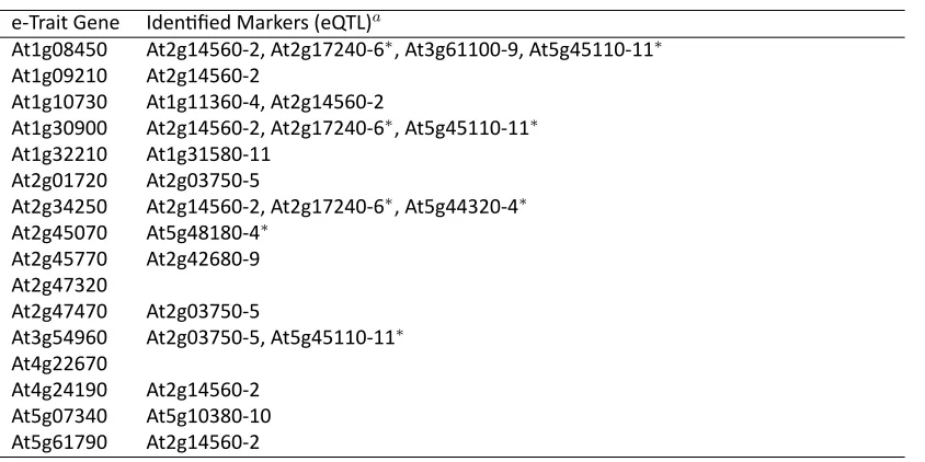
Table S2 summarizes the markers (eQTL) iden fied by the single-trait single-marker approach for each of the 16 e-trait genes. While
some of the markers are close to the 16 genes in the e-trait data, we may be interested to know which of the eQTL are actually from
the 16 e-trait genes, and which are not. Markers that are at least 10 cM from any of the flanking markers of the 16 e-trait genes are
starred in table S2.
Table S2Markers (eQTL) that were iden fied for each of 16 e-trait network genes at significanceα= 0.05by the single-trait single-marker approach
e-Trait Gene Iden fied Markers (eQTL)a
At1g08450 At2g14560-2, At2g17240-6∗, At3g61100-9, At5g45110-11∗
At1g09210 At2g14560-2
At1g10730 At1g11360-4, At2g14560-2
At1g30900 At2g14560-2, At2g17240-6∗, At5g45110-11∗
At1g32210 At1g31580-11
At2g01720 At2g03750-5
At2g34250 At2g14560-2, At2g17240-6∗, At5g44320-4∗ At2g45070 At5g48180-4∗
At2g45770 At2g42680-9
At2g47320
At2g47470 At2g03750-5
At3g54960 At2g03750-5, At5g45110-11∗ At4g22670
At4g24190 At2g14560-2
At5g07340 At5g10380-10
At5g61790 At2g14560-2
aMarkers (eQTL) that are at least 10 cM from any of the flanking markers of the 16 e-trait genes are indicated by∗.
5 More on Predefining the Number of Traits
We showed that the permuta on test works well if we select traits from the permuted data in the same way as from the original data.
For instance, we can specify a number and select this number of "best" traits from the permuted dataset and the original dataset when
we perform the permuta on test (method D in the text). When we applied the proposed VSFOP procedure to the real data analysis,
we used non-parametric bootstrap to determine the number of traits and then select this number of traits when we calculated the test
sta s c and performed the permuta on test. Were type I error rates appropriately controlled in this way? We looked at this ques on
using 200 replicate simula ons. In each simula on, we simulated sixteen traits from a mul variate normal distribu on whose mean and
variance-covariance were respec vely equal to the sample mean and variance-covariance (a er adjus ng for QTL effects at
At3g10720-6) of the actual sixteen e-traits, used 1,000 non-parametric bootstrapped samples to determine the number of traits to select from the
simulated dataset, and performed 1,000 permuta ons of the genotypic data at At3g10720-6 to determine the significance thresholds
of the test. Table S3 shows the results of 200 simula ons. We did not see any problem.
Table S3Es mated type I error rates and standard errors (in parentheses)
α 0.1 0.05 0.01
Type I error rate 0.100(0.0212) 0.045(0.0147) 0.020(0.0099)
6 Es mated QTL Effects and Residual Correla ons
Figure 1 contains lots of informa on. Rather than extensively explore it, we were interested to look at QTL effects and residual
correla-ons for some traits at a few markers, including traits 2, 3, 12 and 16 at marker 3, trait 5 and 8 at marker 10, traits 2, 6 and 9 at marker
26, and traits 1, 4 and 9 at marker 27. The results are as follows.
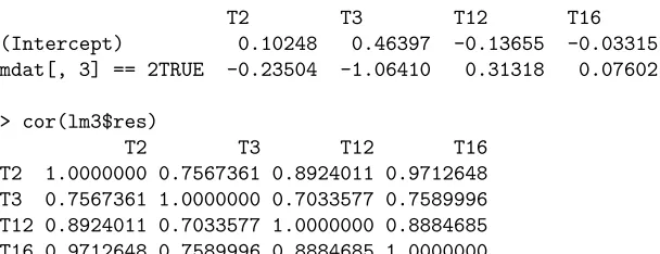
#*** traits 2, 3, 12 and 16 at marker 3 *****************
> lm3<- lm(scale(traits[,c(2,3,12,16)],center=FALSE)~(mdat[,3]==2)) > lm3
Call:
lm(formula = scale(traits[, c(2, 3, 12, 16)]) ~ (mdat[, 3] == 2))
Coefficients:
T2 T3 T12 T16
(Intercept) 0.10248 0.46397 -0.13655 -0.03315 mdat[, 3] == 2TRUE -0.23504 -1.06410 0.31318 0.07602
> cor(lm3$res)
T2 T3 T12 T16
T2 1.0000000 0.7567361 0.8924011 0.9712648 T3 0.7567361 1.0000000 0.7033577 0.7589996 T12 0.8924011 0.7033577 1.0000000 0.8884685 T16 0.9712648 0.7589996 0.8884685 1.0000000
#*** traits 5 and 8 at marker 10 ******************** > lm10<- lm(scale(traits[,c(5,8)])~(mdat[,10]==2)) > lm10
Call:
lm(formula = scale(traits[, c(5, 8)]) ~ (mdat[, 10] == 2))
Coefficients:
T5 T8
(Intercept) 0.61734 0.01505
mdat[, 10] == 2TRUE -1.18417 -0.02886
> cor(lm10$res)
T5 T8
T5 1.0000000 0.8459121 T8 0.8459121 1.0000000
#*** traits 2, 6 and 9 at marker 26 ***************** > lm26<- lm(scale(traits[,c(2,6,9)])~(mdat[,26]==2)) > lm26
Call:
lm(formula = scale(traits[, c(2, 6, 9)]) ~ (mdat[, 26] == 2))
Coefficients:
T2 T6 T9
(Intercept) -0.3548 -0.3690 0.1083 mdat[, 26] == 2TRUE 0.6869 0.7142 -0.2096
> cor(lm26$res)
T2 T6 T9 T2 1.0000000 0.7080602 0.7220022 T6 0.7080602 1.0000000 0.6598618 T9 0.7220022 0.6598618 1.0000000
#*** traits 1, 4 and 9 at marker 27 ***************** > lm27<- lm(scale(traits[,c(1,4,9)])~(mdat[,27]==2)) > lm27
Call:
lm(formula = scale(traits[, c(1, 4, 9)]) ~ (mdat[, 27] == 2))
Coefficients:
T1 T4 T9
(Intercept) -0.6073 -0.6078 0.1468 mdat[, 27] == 2TRUE 1.1046 1.1056 -0.2670
> cor(lm27$res)
T1 T4 T9
T1 1.0000000 0.9225975 0.4170457 T4 0.9225975 1.0000000 0.3705381 T9 0.4170457 0.3705381 1.0000000
Take the first example to explain the output. "traits" was a variable for the trait data with each column being a trait,
and "mdat" was a variable for the marker data with each column represen ng a marker. R func on "scale" centered each
trait to0and then divided it by its standard devia on. Transformed traits 2, 3, 12 and 16 were then regressed on the third
marker using R func on "lm". "Coefficients" lists the es mated overall mean, "(Intercept)", and QTL effect, "mdat[, 3]",
at the third marker for each of traits 2, 3, 12 and 16 (denoted by "T2", "T3", "T12" and "T16" respec vely). The es mated
QTL effect−0.23504means the transformed phenotype "T2" in an individual with genotype "aa" (coded as 2) was smaller
by0.23504than an individual with genotype "AA" (coded as a value other than 2). R func on "cor" called for pairwise
residual correla ons between the traits.
7 Mul trait Analysis Based on Clustering
The e-traits are all posi vely correlated with the correla on ranging from 0.023 to 0.960. Figure S2 displays hierarchical
clustering, based on correla ons of the sixteen e-traits. Using a cutoff 0.75 results in seven clusters. We analyzed each
cluster using the mul trait approach. Figure S3 shows the results of the analysis. The plo ed sta s cs wereT˜2 k =
T2 k ×
v
vk (k= 1,2,· · ·,7), whereT 2
k was the Hotelling'sT2in mul trait analysis of thek-th clustered traits,vkwas the
0.05 genome-wide threshold ofTk2andvwas the minimum ofv12, v22,· · · , v27.
Figure S2Hierarchical clustering of the sixteen e-traits, based on correla ons of the traits, using complete linkage
Figure S3Results from mul trait analysis of seven clusters of the e-traits. The horizontal line indicates the 0.05 significance threshold adjusted for mul plicity of clusters and markers. Each ver cal sec on displays one chromosome.
8 Single-trait Analysis Using Principal Components
We calculated the principal components (PCs) that were based on the variance-covariance of the sixteen e-traits. Figure
S4 displays the percentage of the total variance explained by the firstk(k= 1,2,· · · ,16)PCs. The first four PCs account
for more than 92% of the total variance. We then analyzed the PCs separately. Figure S5 displays the results. Addi on
of a PC other than the first four does not seem jus fiable from figure S4; however, the seventh and eighth ones, which
respec vely account for 0.88% and 0.91% of the total variance, effec vely iden fied QTL.
Figure S4Percentage of variance explained by the firstk(k= 1,2,· · · ,16)principal components
Figure S5Results from single-trait analysis of sixteen principal components of the e-traits. The horizontal line is the threshold at the significance levelα = 0.05, adjusted for mul plicity of both traits and markers. Each ver cal sec on represents one chromosome.
9 Disclose Most Likely Associated Traits via Variable Selec on
There are about twenty-three thousand genes in theArrayExpressdatabase with ID "E-TABM-126". We were tempted to
inves gate all those genes but chose to study the sixteen in a known network. This small set was ideal for us to develop
and evaluate methodology whereas the en re set might not.
In prac ce, it may be more helpful to iden fy a small number rather than a large number of traits that are most
likely associated with a locus. The proposed VSFOP procedure is a useful tool for this purpose. As we observed, this
procedure tended to select a "good" trait along with a "bad" one if the QTL effect was large on some traits. It is not
difficult to pick out the "good" candidate(s). Then we can repeat the process to select the next "good" one(s) from the
remaining traits and so on. This process would be powerful but computa onally challenging. Instead, we employed the
backward elimina on procedure using the Hotelling'sT2test sta s c and a cutoff 17.92879, which was es mated from
10,000 permuted samples and was expected to control the chance of selec ng a trait under 0.05 if there was no QTL on the
genome. We selected a subset of traits (if any) and then picked out the "best" one(s), and repeated this process. We should
be cau ous about undesired results. For instance, at marker 26, the trait combina on {2,6,9} (T{22,6,9}(26) = 114.17) was more favorable than {2,9} (T{22,9}(26) = 87.88) or {6,9} (T{26,9}(26) = 78.22) and even more favorable than {2,6} (T{22,6}(26) = 34.48), and therefore we might get a "bad" choice {9} if we looked for the largest condi onal contribu on. Table S4 displays the result. The order and grouping in table S4 ma er. For instance, at marker 27 we selected trait 1 in
the first round and traits 7 and 14 in the fi h round. The need for mul ple-round search reflects the known fact that the
power of mul trait analysis depends on both the QTL effects and the correla on structure. Note that table S4 provides
more than the single-trait analysis.
However, table S4 may not be desirably available from a full joint analysis of all the 16 traits. We may a empt to look
at es mated QTL effects from a full joint analysis to spot relevant traits if there are only two genotypes at a locus and the
traits are scaled to have the same standard devia on. More formally, we can look at the Wald sta s cs, which proves to
be equivalent to single-trait analysis and thus may not be able to deliver desired results. Alterna vely, we can formally
test the QTL effects via full joint analyses. In such a case, issues we set aside for now include which effects are tested first
and which are tested together. Unfortunately, this might not produce desired results either. Take marker 3 as an example.
Table S4 indicates traits 3, 12 and 2 were relevant. Trait 3 was obvious from the single-trait analysis. Variable selec on also
led to traits 2 and 12. Actually,T{22,12,16}(3) = 132.88,T{22,12}(3) = 73.66,T{22,16}(3) = 88.22,T{212,16}(3) = 15.55,
T2
{2}(3) = 2.89,T 2
{12}(3) = 5.19, andT 2
{16}(3) = 0.30. However, only trait 3 was tested to have a QTL if we jointly analyzed all the 16 traits or all but trait 3 (Table S5). Neither trait 2 nor trait 12 was iden fied as relevant by joint analysis
of traits 2, 12 and 16, traits 2 and 12, traits 2 and 16, or traits 12 and 16 (Table S6). Here might be a possible explana on:
the rela onship between QTL effects and correla on structure weighs in a joint analysis, and the impact of a small change
in QTL effect on a single trait is limited; traits 2 and 12 failed to be iden fied as relevant by joint analysis because the
puta ve QTL had small effects on them.
Finally, we point out that the backward elimina on outperforms the forward selec on. If the forward selec on is
employed, it is be er to over select a subset and then perform the backward elimina on on the subset. What if we have
thousands of traits? We might split them into smaller subsets, employ the backward elimina on to filter "trivial" yet
non-informa ve traits out of the subsets and proceed with the remaining traits. To sum up, there is lots to explore in this
research area.
Table S4Traits most likely associated with the marker
Mark
er
Inde
x
Selected Traits Mark
er
Inde
x
Selected Traits
1 {3} {12} {2} 49
2 {3} {12} {16} {14} {11} {1} 50
3 {3} {12} {2} 51
4 {3} {5} {16} {12} 52
5 {3} {12} {5} {16} 53
6 {3} {5} {2} 54 {1}
7 {5} {3} {16} 55 {1}
8 {5} {3} 56
9 {5} {12} {16} 57
10 {5} {12} 58
11 {5} 59
12 {5} 60
13 {5} 61
14 {5} 62
15 {5} 63
16 {5} 64
17 65
18 66
19 67
20 68
21 69
22 70
23 71
24 {6} {7} {1} {4} 72
25 {6} {1} {2} {11} {4} {7} {12} {16} {14} 73
26 {2,6} {1} {4} {16} {14} {11} {12} {7} {15} {13} 74 27 {1} {4} {2} {16} {7,14} {3,6} {12} {11} {15} {13} 75
28 {1} {2} {14} {4} {16} {6} {7} {12} {11} {9} 76 {15}
29 {1} {4} {2} {16} {14} {7} {6} {12} {9} 77 {15}
30 {1} {9} {4} 78 {15}
31 {1} {4} {9} {16} {7} {2} {12} 79 {15}
32 {9} {1} {4} {7} {16} {12} {2} 80 {15}
33 {1} {9} {4} {8} {11} {10} {7} {15} 81 {15}
34 {9} {1} {11} 82 {15}
35 {9} {11} {14} 83
36 {9} {11} 84
37 {9} {11} 85 {4}
38 {9} 86 {4} {1}
39 {9} 87 {4} {11} {1} {14} {8} {12} {7}
40 88 {4} {1} {7} {8} {12} {11} {14} {15} {16} {13} {2}
41 89 {1} {4} {8} {7} {12} {14} {11} {13} {2} {15} {16}
42 90 {4,8} {1} {7} {12} {11}
43 91 {4} {1} {12} {7} {8}
44 92 {4} {1} {12} {8}
45 93 {8}
46 94
47 95
48
Table S5Likelihood ra o test sta s c for QTL on each of the 16 traits at marker 3, either using all 16 traits ("Yes") or all but trait 3 ("No")
Include T3 T1 T2 T3 T4 T5 T6 T7 T8
Yes 2.9700 2.8954 69.2438 2.1043 0.3108 2.0848 1.7316 5.4177
No 2.9700 2.8958 NA 2.1041 0.3111 2.0844 1.7316 5.4297
Include T3 T9 T10 T11 T12 T13 T14 T15 T16
Yes 1.7386 1.2745 1.4045 5.1700 1.8908 0.3533 0.8362 0.2973
No 1.7388 1.2927 1.4047 5.1702 1.8908 0.3535 0.8366 0.2972
Table S6Likelihood ra o test sta s c for QTL on single traits at marker 3 in joint analysis of traits 2, 12 and 16, 2 and 12, 2 and 16, or 12 and 16
T2 T12 T16
T2, T12 and T16 2.8969 5.1739 0.2986
T2 and T12 2.8991 5.1755 NA
T2 and T16 2.8972 NA 0.2989
T12 and T16 NA 5.1755 0.3008
10 Analysis of the 66 E-Traits
For all the 66 e-traits used in simula ons, we repeated the analysis that resulted in Figure 1 in the text. The results are
displayed in Figure S6. This example confirms that our proposed method is promising. Again, we do not need to select
many traits to detect QTL.
Figure S6Mapping profiles for single-trait analysis of the 66 traits (A) and mul trait analysis of selected traits versus that of all 66 traits (B), and number of selected traits (C). The horizontal lines are 0.05 significance thresholds adjusted for all the markers (and all the traits in the case of single-trait analysis). Each ver cal sec on displays one chromosome.
References
R , A. C., 1993 The contribu on of individual variables to hotelling'st2, wilks'sλ, andr2. Biometrics49: 479--489.