Empirical Analysis of Image Compression
through Wave Transform and Neural Network
1. Amjan Shaik, CSE, Ellenki College of Engineering and Technology(ECET), Patelguda,Hyderabad ,India. 2. Dr.C.R.K Reddy, CSE, Chaitanya Bharathi Institude Of Technology(CBIT), Gandipet, Hyderabad, India. 3. Syed. Azar Ali, IT, Muffakham Jah College of Engineering and Technology(MJCET), Bajara Hills, Hyderabad, India.
Abstract: Images have large data quantity, for storage and transmission of images, high efficiency image compression methods are under wide attention. In this Paper we proposed and implemented a wavelet transform and neural network model for image compression which combines the advantage of wavelet transform and neural network. Images are decomposed using Haar wavelet filters into a set of sub bands with different resolution corresponding to different frequency bands. Scalar quantization and Huffman coding schemes are used for different sub bands based on their statistical properties. The coefficients in low frequency band are compressed by Differential Pulse Code Modulation (DPCM) and the coefficients in higher frequency bands are compressed using neural network. Using this scheme we can achieve satisfactory reconstructed images with increased bit rate, large compression ratios and PSNR. To find the high compression ratio, Peak Signal to Noise ratio (PSNR) with increased bit rate by implementing the Discrete Wavelet Transform (DWT), DPCM and Neural Network. Image compression using cosine transform results a blocking artifacts, where as in image compression using wavelet transform over comes drawbacks associated with cosine transform, using neural network we reduce mean square error. Empirically analyze through Mat Lab and our software tool .We are also calculated and analyzed[12,13] the OO Metrics in this paper.
Keywords: Image Compression, Discrete Wavelet Transform, Neural Network, OOD Metrics.
1.INTRODUCTION
Image compression is a part of large context where different types and size of images are compressed using different methodologies. Computer file format designed primarily to store scanned documents, especially those containing a combination of text, line drawings, and photographs. Image compression uses technologies such as image layer separation of text and background/images, progressive loading, arithmetic coding, and lossy compression for bitonal (monochrome) images. The initial image is first separated into three images: a background image, a foreground image, and a mask image. The background and foreground images are typically lower-resolution color images (e.g., 100dpi); the mask image is a high-resolution bi-level image (e.g., 300dpi) and is typically where the text is stored. Uses JB2 encoding method identifies nearly-identical shapes on the page, such as multiple occurrences of a particular character in a given font, style, and size[3,4]. It compresses the bitmap of each unique shape separately, and then encodes the locations where each shape appears on the page. Optionally, these shapes may be mapped to ASCII codes, If this mapping exists, it is possible to
select and copy text. If it doesn’t map then resultant image may be distorted and blur. Using this scheme satisfactory reconstructed image with lossy bit rate, small compression ratios and low PSNR (peak signal to noise ratio) is expected.
1.1 Image compression Techniques
Image compression is a key technology in the development of various multi-media computer services and telecommunication applications such as video conferencing, interactive education and numerous other areas. Image compression techniques aim at removing (or minimizing) redundancy in data, yet maintains acceptable image reconstruction. A series of standards including JPEG, MPEG and H.261 for image and video compression have been completed. At present, the main core of image compression technology consists of three important processing stages: pixel transforms, vector quantization and entropy coding. The design of pixel transforms is to convert the input image into another space where image can be represented by uncorrelated coefficients or frequency bands[2,7].
Recent advances in signal processing tools such as wavelets opened up a new horizon in sub band image coding. Studies in wavelets showed that the wavelet transform exhibits the orientation and frequency selectivity of images. Neural networks approaches used for data processing seem to be very efficient, this is mainly due to their structures which offers parallel processing of data and, training process makes the network suitable for various kind of data. Sonhera et al have used a two layered neural network with the number of units in the input and output layers the same, and the number of hidden units smaller. The network is trained to perform the identity mapping and the compressed image is the output of the hidden layer. Arozullah et al presented a hierarchical neural network for image compression where the image is compressed in the first step with a given compression ratio; then the compressed image is itself compressed using another neural network[8,10]. Hussan et al proposed a dynamically constructed neural architecture for multistage image compression. In this architecture the necessary number of hidden layers and the number of units in each hidden layer are determined automatically for a given image compression quality. Gersho et al have used Kohonen Self-organizing Features Map (SOFM) for designing a codebook for vector quantization of images.
2. IMAGE COMPRESSION
Image compression addresses the problem of reducing the amount of data required to represent a digital image. The underlying basis of the reduction process is the removal of redundant data. From a mathematical viewpoint, this amounts to transforming a 2-D pixel array into a statistically uncorrelated data set. The transformation is applied prior to storage or transmission of the image. At some later time, the compressed image is decompressed to reconstruct the original image or an approximation of it. The term data compression refers to the process of reducing the amount of data required to represent a quantity of information. A clear distinction must be made between the information and data. They are not same. In fact data are the means by which information is conveyed. Various amounts of data may be used to represent the same amount of information. For example one story can explain in two different languages (data), hear information is same language (data) is different, in total story any one word may be same in two languages that word is redundant, which is known as data redundancy.
Data redundancy is central issue in digital image compression. It is not an abstract concept but a mathematically quantifiable entity. If and denotes number of information carrying units in two data sets that represents the same information, the relative data
redundancy of the first data set (the one characterized by n ) can be defined as
...………1
Where , is compression ratio is
………2
In digital image compression, three basic data redundancy can be identified and exploited (a) coding redundancy, (b) interpixel redundancy, and (c) psychovisual redundancy (Digital Image processing by Rafael C.Gonzalez and Richards E. Woods). Data compression is achieved when one or more of these redundancies are reduced or eliminated. In this thesis image compression is achieved using coding redundancy.
a. Coding redundancy:
In digital image processing the technique for image enhancement by histogram processing on the assumption that the gray levels of an image are random quantities. In this thesis we give similar formulation to show the gray level of an image also can provide a great deal of insight into the construction of codes to reduce the amount of data used to represent it. The mathematical equations of coding redundancy is
k=0,1,2,3,……..L-1 ……….3
…………...4
Where L is number of gray levels, is number of times that the kth gray level appears in the image and n is the number of pixels in the image. is the discrete random variable in the interval [0, 1], length of the bit stream to represent each variable of and is the average number of bits required to represent each pixel.
b. Interpixel redundancy:
should be transformed into another, generally "non-visual" representation. For our example above, such representation may be the value of leftmost top pixel along with 1-D array of differences between adjacent pixels. Transformations used to reduce the interpixel redundancies are called mapping. Since in this paper we deal only with lossless compression, the mappings, which will be considered further, will be reversible.
c. psycho visual redundancy:
It is known that the human eye does not respond to all visual information with equal sensitivity. Some information is simply of less relative importance. This information is referred to as psycho visual redundant and can be eliminated without introducing any significant difference to the human eye. The reduction of redundant visual information has some practical applications in image compression. Since the reduction of psycho visual redundancy results in quantitative loss of information, this type of reduction is referred to as quantization. The most common technique for quantization is the reduction of number of colours used in the image, thus colour quantization. Since some information is lost, the colour quantization is an irreversible process. So the compression techniques that used such process are lossy. It should be noted that even if this method of compression is lossy, in situations where such compression technique is acceptable the compression can be very effective and reduce the size of the image considerably.
2.1Error criteria:
To judge the performance of a lossy compression technique we need to decide upon the error criteria. The error criteria commonly used may be classified into two broad groups: (a) Objective criteria, (b) Subjective criteria.
Objective criteria: When the level of information loss can be expressed as function of the original image or input image and compressed and subsequently decompressed output image, it is said to be based on an objective criteria. A good example is root mean square error between an input and output image. Let f(x, y) is
the input image and output image or
decompressed output image. For any value of x and y
error e(x, y) between f(x, y) and can be defined as
f(x, y) = ..………5
So that the total error between the two image is
…… 6 Where image are of size M*N the root mean square error
, between f(x, y) and then is the square root of the squared error average over the M*N array or
=
……….7
A closely related objective criterion is the mean square signal to noise ratio of the compressed-decompressed image. If is consider as sum of original f(x, y)and noisy image e(x, y) the mean square signal to noise ratio of the output image,
= …...8
The root mean square(rms) value of the signal to noise ratio, denoted by
Subjective criteria: The subjective error measure is performed as follows. The original image and the reconstructed image are shown to a large group of examiners. Each examiner assigns grade to the reconstructed image with respect to the original image. These grades may be drawn from a subjective side, divide as, and say excellent, good reasonable poor and unacceptable. However the scale can of course be dividing into coarser or finer bins. Finally, based on grade s assigned by the entire examiner, an overall grade is assigned to the reconstructed image. Complement of this grade gives an idea of the subjective error.
3. IMAGE COMPRESSION MODELS
The three general techniques for image compression are given in section 3. However these three techniques are combined to form a practical image compression system. In the figure.1 shows the general compression system model consist of encoder path f(x, y) is the input image which is fed to the source encoder which creates set symbols of input data, these input data is transformed over the channel. The decoder receives the data through the channel and reconstructed from decoder. If
is equal to input image then it is error free if not it is lossy image (distorted image). Both encoder and decoder consist of sub block. The encoder consist source encoder which reduces the redundancy and channel encoder which increases the immunity of the source encoders output. The decoder part consists of channel decoder and source decoder. If the output image is noise free the channel encoder and source decoder is eliminated and general encoder and decoder becomes source encoder and decoder respectively.
3.1 Differential Pulse Code Modulation (DPCM)
prediction and quantizer present in transmitter side and quantizer is eliminated in decoder part of receiver side, hence it is called lossy compression. Gray levels of adjacent pixels are highly correlated for most of images. Thus the autocorrelation function for the picture is used as a measure for coding. If fn-1 is having a certain gray
level then the adjacent pixel fn along the scan line is
likely to have a similar values, where n is the number of pixels in the input image. The pixel gray levels in whole range of 256 values in an image have adjacent pixel difference that is very small in the range 20 gray level values.
DPCM make use of this property as follows: we conceder a pixel fn-1 and based on this observed values,
we predict value of the next pixel fn. Let be the
predicted value of fn and let us subtract this from actual
value fn to get difference (en). The difference (en) will not
the average be significantly smaller in magnitude then the actual magnitude of pixel fn. Consequently we
require fewer quantization levels and thus bits to code the sequence of differences then would be required to code the sequence of pixels.
3.2 Huffman Encoder
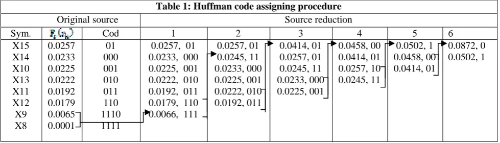
The well known technique for removing the coding redundancy is due to the Huffman (Huffman [1952]). When coding the symbols of an information source i.e. quantized output of DPCM and neural network individually, Huffman coding the smallest possible number of code symbols per source symbols. In terms of noise less coding theorem the resulting code is optimal for a fixed value of n subject to the constraint that the source symbols be coded one at a time. The original source symbols with probability ( Pr( rk ) ) is given in the
Table.1
Step1: Probabilities of source symbol are arranged in descending order, i.e. top to bottom of the look up table 3.
Step2: Adding up the two lowest probability symbols from bottom to top to a single symbol and replace them in next column of source reduction of figure (4.)
Step3: Repeat step1 and step2 until the two probability symbols are obtained
The second step in the Huffman coding is to code each reduced source starting with a smallest source and working back to the original source assigning two binary symbols 0 and 1 in reverse order. From right to left as the reduced source symbol with probability 0.6 was generated by combining two symbols in the reduced source to its left, the 0 used to code it is now assigned to both symbols, and a 0 and 1 are arbitrarily appended to each to distinguish them from each other. This process is then repeated for each reduced source until the original source is reached. The average length of this code is Lavg = (0.0257)(2) + (0.0233)(3) +(0.0225)(3) +
(0.0222)(3) + (0.0192)(3) + (0.0179)(3) + (0.0065)(4) + (0.0001)(4)
=0.3931 bits/symbols.
Finally we required 0.3931 bits/symbols to code the information source.
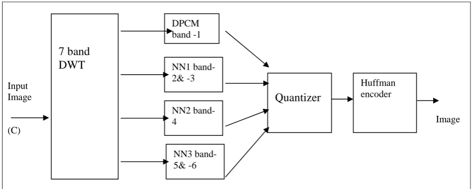
The Huffman’s procedure creates the optimal code for asset of symbols and probabilities subjects to the constraint that the symbols be coded, coding and /or decoding is accomplished in a simple look up table manner. Different frequency sub bands coefficient of a DWT is compressed with DPCM, neural network. Therefore band-1 is compressed with DPCM and band-2 to band-7 are compressed with neural network, band -2 and band-3 has same frequency with different orientation so these two bands are compressed with one neural network, similarly band-5and -6 is compressed with another neural network, frequency coefficient of band-4 does not match with any other bands that’s why it is compressed with separate neural network and band-7 does not contains much information so it is neglected. This compressed information is scalar quantized and then Huffman encoded.
3.3 Complete Image Compression Scheme
Figure 3 shows the block diagram of complete image compression system. First the image is decomposed into different frequency bands these frequency bands are low frequency band and high frequency bands the lowest frequency band represents the one forth of original resolution, is coded using DPCM. The remaining frequency bands are coded using neural network compression scheme.
Table 1: Huffman code assigning procedure
Original source Source reduction
Sym. Cod 1 2 3 4 5 6
X15 X14 X10 X13 X11 X12 X9 X8 0.0257 0.0233 0.0225 0.0222 0.0192 0.0179 0.0065 0.0001 01 000 001 010 011 110 1110 1111
0.0257, 01 0.0233, 000 0.0225, 001 0.0222, 010 0.0192, 011 0.0179, 110 0.0066, 111
Figure 1: Block diagram of implementation of wavelet transform, DPCM, neural network for image compression.
Figure 2: Block diagram of decompression
The low frequency band-1 is compressed with Optimal DPCM which reduces the inter pixel redundancy. Depending upon previous pixel information we can predict the next pixel, the difference between current pixel and predicted pixel is given to optimal quantizer which reduces the granular noise and slop over lode noise. Finally we get the error output from DPCM the corresponding image is shown in fig (1), these error values are scalar quantized.
The Human Visual System (HVS) has different sensitivity to different frequency components, for this reason we are going for neural network, neural networks of different sizes must be used to allow for different reconstruction quality, resulting in different compression ratios for the various frequency bands.
After the wavelet coefficient are compressed using either DPCM or by using neural network. The output of the DPCM and neural network are scalar
quantized where the values of entire kx1 hidden vectors are scalar quantized at once. The results are given in the next section. Finally, the quantized values are Huffman encoded.
Fig:3 Image of band-1 Fig:4Image of band-2
Fig:5 Image of band-3 Fig:6 Image of band-4
Input
Image compressed
Image (C)
C
7 band
DWT
DPCM band -1
NN1 band-2& -3
Quantizer
Huffman encoder
NN2 band-4
NN3 band-5& -6
Huffman decoder
De-quantizer
7 band
DWT
DPCM band -1
NN1 band-2& -3
NN2 band-4
NN3 band-5& -6
3.4 Image Decompression scheme
The block diagram of decompression scheme for compressed image (compressed bit stream) is shown in figure 7. The output of the Huffman encoder is given to Huffman decoder, these reconstructed bit streams are dequantized, the output of the dequantized values are frequency band-1 to band-7, band-1 is compressed low frequency band and ban-2 to band-7 are compressed high frequency bands. The compressed low frequency components are given to inverse DPCM (IDPCM) in inverse DPCM quantization will not be present. The compressed frequency bands are given to output layer of the neural network, and then we get reconstructed sub bands. These reconstructed sub bands are given to Inverse Discrete Wavelet Transform (IDWT), the output of the IDWT is our desire output i.e. reconstructed image.
Figure: 7 Reconstructed image
3.5 Use of Frequency band for Compression
Input image (cameraman image ) of size 256 X 256 is decomposed into seven frequency bands with different resolutions is compressed with DPCM, and neural network, these compressed image is scalar quantized and the quantized bits ire Huffman encoded.
4. RESULTS OF IMPLEMENTATION WT AND NN
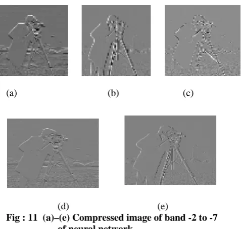
The experiment evaluates the effect of discreet Haar wavelet filters on the quality of the reconstructed image. In the experiment where conducted using cameramen image of size 256 X 256with 28=256 gray levels. The image was decomposed using Haar wavelet transform. Coefficients of bant-1 see figure 2 is coded with differential pulse code modulation (DPCM), coefficients of band -2 and band -3 are coded using neural network which has eight input units and eight output units, and six hidden units, i.e., a 8 - 6 - 8 neural network. To compresses the coefficients of band-4 we use an eight input units and eight output units and four hidden units i.e., 8 - 4 - 8 neural network and band 5 and 6 uses sixteen input units and sixteen output units, and one hidden unit i.e., 16 – 1 – 16 neural network these compressed information is scalar quantizer and the coefficients of hidden layer is encoded with Huffman encoder the compressed image and original image is shown in figure. The results was evaluated by PSNR and
compression ratio (CR) defined for the image of size M X M as
PSNR = ……9
CR = …...…. 10
Where 255 is peak signal value, and are the input image pixel and output image pixels respectively. The input and reconstructed figures are shown in figures 8-10.
Fig 8: Camera man Fig 9: Reconstructed input image image.
Fig 10: Compressed image Input image
of DPCM
(a) (b) (c)
(d) (e)
Fig : 11 (a)–(e) Compressed image of band -2 to -7 of neural network
4.1 Results:
Figure 12: Mat Lab editor to run code
Figure13: Browsing And Opening GUI File
(Figure14: Resultant image of camera man after
compression of size 64x64)
(Figure15: Camera man image of size 256 x256 is input for compressions)
5. CONCLUSION
In this Paper we used techniques such as wavelet transforms, DPCM and Neural Network for image compression. we discussed complete image compression and decompression scheme. First input image is decomposed using DWT these decomposed frequency bands are low frequency band and high frequency bands, the low frequency band are compressed with DPCM and high frequency bands are compressed with neural network and encoded with Huffman encoder. The compressed bit stream is decompressed using DPCM and DWT. Compared to the neural network applied on the original image wavelet based decomposition improved dramatically the quality of reconstructed images. Wavelet decomposition eliminates blocking effects associated with DCT. This application may be further extended for automatic compression of data and images to large extent where transfer of data over web is most effective and convenient for the users. In this application data is secure and will not loose its efficiency. And more over it can be used in Bar code creation to identify any product or person. We are discussed the importance[12,13] of OOD Metrics and measured through our software tool in this paper.
ACKNOWLEDGEMENTS
REFERENCES:
[1] J. W. Woods and S. D. O’Neil, , “Sub band coding of images,” IEEE Trans. Acoust., Speech, Signal Processing, vol. 34, 1986, pp. 1278–1288.
[2] S. G. Mallat, ,“A theory for multi resolution signal decomposition: The wavelet representation,” IEEE Trans. Pattern Anal. Machine Intell., vol. 11, 1989, pp. 674–693.
[3] Ronald E.Crochiere and Lawrence R. Rabiner, multirate digital signal processing Printi- Hall, Englewood Cliffs, NJ, 1983.
[4] S. G. Mallat, , “Multi frequency channel decomposition of images and wavelet models,” IEEE Trans. Acoust., Speech, Signal Processing, vol. 37, 1989, pp. 2091–2110.
[5] P. C. Millar, , “Recursive quadrature mirror filters—Criteria specification and design method,” IEEE Trans. Acoust., Speech, Signal Processing, vol. 33, 1985, pp. 413–420.
[6] B. Ramamurthi, A. Gersho. “Classified Vector Quantization of Images” IEEE Transactions on Communications, Vol.Com-34, No. 11, 1986,
[7] M. Mougeot, R. Azeneott, B. Angeniol, “Image compression with back propagation: improvement of the visual restoration using different cost functions” neural networks, vol 4, No 4 1991, pp 467-476 [8] M. Antonini, M. Barlaud, P. Mathieu, and I. Daubechies, “Image coding using wavelet transform,” IEEE Trans. Image Processing, vol. 1, 1992, pp. 205–220.
[9] D. Esteban and C. Galand, “Applications of quadrature mirror filters to split band voice coding schemes,” in Proc. IEEE Int. Conf. Acoustics, Acoustics, Speech and Signal Processing, Washington, DC, 1979, pp. 191–195.
[10] Manphol s. Chin and M. Arozullah, ‘‘Image compression with a hierarchical neural networks”, IEEE Trans. Aerospace and Electronic Systems, vol. 32, no 1. 1996,
[11] M. H. Hassan, H. Nait Charif and T. Yahagi, , “A Dynamically Constructive Neural Architecture for Multistage Image Compression”, Znt. Conference on Circuits, Systems and Computer, (IMACS-CS’98). 1998.
[12].Amjan Shaik, Dr.C.R.K.Reddy, M.Bala, “An Empirical Validation of Object Oriented Design Metrics in Object Oriented Systems International Journal of Emerging Trends in Engineering and Applied Sciences(JETEAS)Volume.1, No.2, Page 211-219, ISSN: 2141–7016, December, 2010.
[13].Amjan Shaik, Dr.C.R.K.Reddy, M.Bala ,“Metrics for Object Oriented Design Software Systems: Survey”International Journal of Emerging Trends in Engineering and Applied Sciences(JETEAS),Volume.1, No.2,Page 189-197,ISSN: 2141–7016, December, 2010.
ABOUT THE AUTHORS:
Amjan Shaik is working as a Professor and Head, Department of Computer Science and Engineering at Ellenki College of Engineering and Technology (ECET), Hyderabad, India.He has received M.Tech. (Computer Science and Technology) from Andhra University. Presently, he is a Research Scholar in JNTUH. He has been published and presented good number of technical and Research papers in International, National Conferences and International Journals. His main research interests are Software Engineering, Software Metrics and OOAD.
Dr.C.R.K. Reddy is working as a Professor and Head, Department of Computer Science and Engineering at Chaitanya Bharathi Institute of Technology (CBIT),Hyderabad, India. He has received M.Tech.( Computer Science and Engineering ) from JNTUH, Hyderabad and Ph.D in Computer Science and Engineering from Hyderabad Central University (HCU). He has been published and presented wide range of Research and technical Papers in National , International Conferences, and National , International Journals. At present 8 Research Scholars are doing Ph.D under his esteemed guidance. His main research Interests are Program Testing , Software Engineering , Software Metrics and Software Architectures.