Reynolds’ Turbulence Solution
Bo-Hua Sun11
Institute of Mechanics and Technology & School of Civil Engineering, Xi’an University of Architecture and Technology, Xi’an 710055, China
http://imt.xauat.edu.cn email: [email protected]
(Dated: August 6, 2019)
The study found an error in current literature, including numerous textbooks, about the number of independent unknowns in the Reynolds stress tensor and/or in Reynolds-averaged Navier-Stokes equations (RANS). Current literature claims that the Reynolds stress tensor has six unknowns; however, this article shows that the Reynolds stress tensor only has independent three unknowns, which are functions of the three components of fluctuation velocity. This research discovers that the misconception about the number of independent unknowns in the RANS could stem from misinter-preting the Reynolds stress tensor. The misconception has hampered the development of turbulence for longtime. In order to find a way out of this difficult situation, we return to the time of Reynolds in 1895 and revisit Reynolds’ averaging formulation of turbulence. The present investigation can be considered as a renaissance of Reynolds’ work in 1895, which might shed light on the well-known closure problem of turbulence, and help to understand the puzzle of the turbulence closure problem that has eluded scientists and mathematicians for more than a century.
Keywords: Turbulence, number of independent unknowns, Reynolds stress tensor, RANS, turbulence closure problem
I. INTRODUCTION
/I am an old man now, and when I die and go to heaven there are two matters on which I hope for enlightenment. One is rela-tivity/quantum mechanics/quantum electro-dynamics [in various versions], and the other is turbulent motion of fluids. About the for-mer I am rather optimistic.0–Horace Lamb [1]
You’re on a airplane when you feel a sudden jolt. Out-side your window nothing seems to be happening, as yet the plane continues to rattle you and your fellow passen-gers as it passes through turbulent air in the atmosphere, and yet, turbulence is ubiquitous, springing up in virtu-ally any system that has moving fluids. That includes that airflow in your respiratory tract. The blood mov-ing through your arteries. And the coffee in your cup as you stir it. Clouds are governed by turbulence, as are waves crashing along the shore and the gusts of plasma in our Sun. Understanding precisely how this phenomenon works would have a bearing on so many aspects of our lives [2–28, 30–42, 44–53, 55–65].
The turbulence phenomenon is one of the greatest pre-vailing unsolved mysteries of physics. After more than a century of studying turbulence, we’ve found a few an-swers on how it works, and affects the world around us. Most scientists argue that this will be by achieved relying on statistics and increased computing power. Extremely high-speed computer simulations of turbulent flows may help to identify patterns that lead to a theory that or-ganizes and unifies predictions for different situations. Other scientists state that the phenomenon is so com-plex that such a full-fledged theory will not be possible
[2–28, 30–42, 44–53, 55–65].
In respect of the turbulence problem, a myriad of ten-tative theories have been proposed and each with its own doctrines and beliefs, which often focused on particular experiments; however, there is not much in the way of a coherent theoretical framework [6, 8–17, 39–41]. Tur-bulence is a unique subject, which engineers, mathemati-cians and physicists view differently [36]. Many engineers promote the use of semi-empirical models of turbulence [36], while mathematicians advocate the use of purely statistical models [5, 7, 30, 31, 45–48, 55, 56], the reno-malization model [34], and the formalism of chaos theory and fractals [49–51].
In 1972 a new chapter was launched in turbulence the-ory: [52] demonstrated that it was possible to perform di-rect numerical simulation (DNS) of a fully turbulent flow. It is important to understand that DNS does not require any turbulence model to parameterize influence of the turbulent eddies. Rather, every eddy, from the largest to the smallest, is computed. From a technical perspective, the turbulence can be solved by DNS if computers have infinite speed. However, a huge chasm remains between what the engineer needs to know, and what can be re-alized by DNS, using current computers. Even if DNS can assist to solve turbulence issues and problems, one still requires turbulence modelling to acquire a physical understanding of it [37].
Although the above-mentioned professionals have dif-ferent views about turbulence, there is consensus that the deterministic Navier-Stokes equation probably contain-s all the information about turbulence [6]. Turbulence prediction can be attained by understanding solutions to the Navier-Stokes equations [5, 6, 8–25, 27, 28, 30– 42, 44–53, 55–62, 64, 65]. Navier [21] and Poisson [22] first obtained these equations, which were finally shown
by St. Venant and Sir Gabbriel Stokes [23, 24] on vari-ous considerations as to the mutual action of the ultimate molecules of fluids [19, 20]. Hence, numerous works have been reported on various aspects of the Navier-Stokes equations. [6, 8–19, 25, 28, 39–41].
The article adopts Reynolds’s deterministic view on the turbulence [19], and revisits the Reynolds-averaged Navier-Stokes equations (RANS). This article deals with a basic problem in turbulence analysis, namely the num-ber of unknowns in the Reynolds stress tensor. This is obviously a fundamental question in fluid mechanics as well. The research in this paper reveals that the RAN-S only has three independent unknowns instead of six, is stated in current literature, including textbooks [8– 15, 18, 30–33, 39–41].
Although the Reynolds-averaged-Navier-Stokes-Equations (RANS) have been formulated for more than 120 years, much of current literature and standard turbulence textbooks have incorrect information about the number of unknowns and this prevented solving the turbulence problem. Hence, if the number of unknowns are incorrect, no solutions will be possible. This situation must be corrected immediately, else it will be harmful for turbulence studies.
In view of the fact that no essential result on turbu-lence definition has been made, it would probably be fit-ting to return to the beginning of turbulent research, that is, in 1895, to study Reynolds’ seminal studies to redis-cover certain useful information.
The aims of this paper are to revisit Reynolds’ aver-aging formulation of turbulence, and to clarify the num-ber of unknowns in the Reynolds stress tensor and/or in RANS. The paper is organized as follows: following an introduction, we introduce Reynolds velocity decompo-sition and reformulate Reynolds-averaged Navier-Stokes equations in tensorial form; we point out an importan-t quesimportan-tion abouimportan-t importan-the number of independenimportan-t unknowns in both the Reynolds stress tensor and the RANS; we provide three mathematical lemma and evidence about the number of independent unknowns. Finally, the pa-per concludes with pa-perspectives about the future devel-opment of turbulence research.
II. REYNOLDS-AVERAGED NAVIER-STOKES EQUATIONS AND DETERMINISTIC NATURE
From the infinitesimal analysis of the Naviers-Stokes e-quation [43], there are 10 Lie groups have been founded, however there is no one group is suitable to the turbu-lence solution.
In ground-breaking research, Reynolds [19], considered turbulence from a different perspective. Assuming that turbulent motion already exists, he sought to establish a criterion, which decides whether the turbulent character will increase or diminish, or remain stationary [20].
From experiments, Reynolds [19], discovered the tur-bulence solution could be expressed in the sum of mean
and fluctuation part of velocity field, which is the so-lution not been founded by the Lie group analysis [19]. Reynolds’ solution method is a quite general approach for any nonlinear partial differential equations (PDE), which transfers the PDE to integro-differential equations.
In 1895 Reynolds proposed that flow velocity u and pressurep are decomposed into its time-averaged quan-tities, ¯u, ¯p, and fluctuating quantities, u0, p0; thus, the Reynolds’ decompositions are:
u = ¯u(x) +u0(x, t), (1) p(x, t) = ¯p(x) +p0(x, t), (2)
where coordinates and time are (x, t). According to Reynolds, ¯u represent a mean-motion at each point and u0a motion at the same point as the mean-motion at the point. Therefore, Reynolds called the ¯u mean-motion andu0 relatimean-motion [19]. Both velocity and ve-locity and pressure time-averaging definitions are defined as
¯
u(x) = lim T→∞
1 T
Z t0+T
t0
u(x, t)dt, (3)
¯
p(x) = lim T→∞
1 T
Z t0+T
t0
p(x, t)dt, (4)
whereT is the period of time when the averaging takes place and must be sufficiently large to give meaningful averages to measure mean values. Naturally, the time-fluctuation velocityu0=u−u¯(x), pressurep0 =p−p(¯x); and their time-averaging vanish, namely ¯u0 =0and ¯p0 = 0.
Decomposition causes the Navier-Stokes equation to transform into Reynolds-averaged Navier-Stokes equa-tions (RANS), as follows
ρ∇·( ¯u⊗u¯) +∇p¯ = µ∇2u¯+∇·τ, (5)
∇·u¯ = 0, (6)
where dynamic viscosityµ, gradient operator∇=ei∇i, base vector in the i-coordinateei, and tensor product⊗, and the Reynolds stress tensor is given by
τ(x) =−ρu0⊗u0=−ρ lim T→∞
1 T
Z t0+T
t0
(u0⊗u0)dt, (7)
which reveals that Reynolds stress is apparent, depending on the fluctuating velocity fieldu0.
In order to obtain more information about the Reynolds’ stress tensor, Reynolds [19] derived veloci-ty fluctuation equations, namely the equation (16) in [19]), called the equations of momentum of relativmean-motion at each point. Chou [32] reformulated these e-quations into index-tensorial at form. The ee-quations are presented in below bold-face tensorial form as follows
ρu0,t+ρ∇·( ¯u⊗u0+u0⊗u¯+u0⊗u0) +∇p0
=µ∇2u0+ρlim
T→∞T1 R t+T t ∇·(u
0⊗u0)dt, (8)
These are integral-differential equations governing ¯u,u0 andp0.
In above Eqs.5,6, 10 and 11 and relevant relations, why we express the problem in tensorial format instead of in cartesian components one, it is because that such formu-lations will not reply on any choice of coordinates, there-fore, the results in this paper will be more general and universal. A basic philosophy of modern physics is that the universe does not come equipped with a coordinate system. While coordinate systems are necessary for doing specific calculations, the choice of the coordinate system to use is a matter of convenience, and there is often no ”best” coordinate system. One should strive to write the laws of physics in a manifestly coordinate-independent manner, so one can see what they are really saying and not get distracted by things that might depend on the coordinates [54].
Denoting kinematic viscosityν=µ/ρ, the Eqs.5,6 can be equivalently rewritten in conventional form, namely
¯
u·∇u¯+ limT→∞T1 R t0+T
t0 (u
0·∇u0)dt
=−1
ρ∇p¯+ν∇
2u¯ (10)
∇·u¯ = 0. (11)
These integro-differential equations are called Reynolds-averaged Navier-Stokes equations (RANS), which were the equations (15) in [19] that Reynolds formulated, call-ing them equations of mean-motion at every point. It is clear that the RANS are deterministic equations rather than statistical ones [19, 20].
It is worth pointing out that for the deterministic ve-locity field u(x, t), the Reynolds decomposition in Eqs. 1 and 2 can always be well-defined by Eqs. 3 and 4. In other words, Reynolds decomposition can always be con-structed for any flow motion, regardless of turbulent flow or not.
The governing equations of flows are deterministic, not random. So fundamentally turbulent fields are not ran-dom because their generating dynamics is not ranran-dom [29]. Random is not intrinsic properties of turbulent field while extrinsic ones. It is misleading to consider the essence of turbulence as a random motion, and the flow velocity field u as a statistical function [30]. Be-cause there is consensus on turbulence, namely that the deterministic Navier-Stokes equations contain all the re-quired information about turbulence [6], means that the essence of the flow velocity and its Navier-Stokes equa-tions is deterministic, rather than random. Taylor [30] introduced a statistical approach and attempted to study turbulence from a statistical point of view; however, the approach is merely a mathematical method for solution-s, which cannot change the deterministic nature of flow velocityu and Navier-Stokes equations. In physics, tur-bulence cannot be considered as a random motion simply because it is difficulty to solve. Generally speaking, any mathematical method used for solving a problem should not change the physics of the problem.
III. HOW MANY UNKNOWNS ARE THERE IN THE REYNOLDS STRESS TENSOR AND/OR
REYNOLDS-AVERAGED NAVIER-STOKES EQUATIONS ?
All current literature including textbooks, report that the Reynolds stresses τ have six unknowns (Later we will show that the Reynolds stresses only have three un-knowns instead of six). This traditional understanding has resulted in consensus that there are 10 unknowns as shown in Eqs.5, 6 and/or Eqs.10, 11.
In his 1895 paper [19], Reynolds did not discuss the number of unknowns in the RANS. However, from his presentation we note that he never considered the term ρu0⊗u0 as independent unknowns, while for some cases he proposed explicit expressions for the velocity fluctu-ationu0 on page 149, and equation (50) on page 158 of his paper [19]. For instance, one expression he proposed on page 149 of [19] is:
X Arcos
r
nt+2π a x
and in the section, Expressions for the components of possible relative-mean-motion, he proposed a similar ex-pression on page 15 of [19], as follows:
u0= ∞ X
0
(dαn dy +
dγn
dz cos(nlx) + ( dβn
dy + dδn
dz ) sin(nlx)
,
v0= ∞ X
0
{nαnsin(nlx)−nlβncos(nlx)},
w0= ∞ X
0
{nγnsin(nlx)−nlδncos(nlx)}.
Reynolds also compiled integrations by using the above expressions, for example, equation (58) on page 159 of Reynolds’s research [19], which is shown below:
Z Z
ρu0v0d¯u dydydz
= 1 2
Z Z X
nl
αn dβn
dy −βn dαn
dy
d¯u dy
dydz.
Giving the above expressions means that Reynolds re-garded the velocity fluctuation u0 not only as indepen-dent unknowns but also deterministic quantity (not a random one !). Please see Reynolds research paper [19] for the meaning of the notations in the above expression-s..
Due to limited references, the author does not know who was the first person who proposed the 10-unknowns perception in the RANS. This mistake in classical physics has hampered the development of turbulence.
a matter of fact, these four equations contain more than four independent unknowns. In addition to ¯u and ¯p, there are also the Reynolds stresses τ, which results in the Reynolds-averaged Navier-Stokes equations being un-closed. The closure problem has been considered as the number one topic in turbulence during the past several decades, while scientists and engineers have made many attempts to solve this closure problem, however, no uni-versal modelling has been proposed.
Regarding the RANS closure problem, the curren-t consensus is curren-thacurren-t curren-there are six unknown componencurren-ts in the symmetric Reynolds stress tensor τ, namely τ11, τ12, τ13, τ22, τ23, τ33. However, this research study presents a complete different perspectives. The Reynold-s Reynold-streReynold-sReynold-s tenReynold-sor τ only has three independent unknown-s, which are fully determined by the velocity fluctua-tion components u0i(i = 1,2,3) owing to the fact that the Reynolds stress tensor is simply an integration of a second order dyadic tensor of flow velocity fluctuations rather than a general symmetric tensor.
IV. LEMMA
Following lemmas support the above statement.
Lemma 1 Given two vectors, v(x, t) = viei = v1e1+ v2e2+v3e3 andw(x, t) =wjej=w1e1+w2e2+w3e3, we can define a dyadic tensor v⊗w as follows [66]
v⊗w=viei⊗wjej=viwjei⊗ej
=v1w1e1⊗e1+v1w2e1⊗e2+v1w3e1⊗e3 +v2w1e2⊗e1+v2w2e2⊗e2+v2w3e2⊗e3
+v3w1e3⊗e1+v3w2e3⊗e2+v3w3e3⊗e3. (12)
In general, in the case of v 6= w, the dyadic tensor
v⊗w is a general tensor with 9 components (elements) and has 6 independent unknowns, namely v1, v2 and v3 andw1, w2 andw3, since the 9 components can be fully determined by the 6 independent unknowns.
If v=w, the tensor v⊗w is a 2rd order tensor with 9 components (elements), and have 3 independent un-knowns, namely v1, v2 and v3 and/or w1, w2 and w3, since the 9 components can be fully determined by the 3 independent unknowns.
Lemma 2 Given three vectors,u(x, t) =uiei=u1e1+ u2e2+u3e3 , v(x, t) = viei = v1e1+v2e2+v3e3 and
w(x, t) =wjej =w1e1+w2e2+w3e3, we can define a 3rd order tensorv⊗w as follows
u⊗v⊗w=uiek⊗vkei⊗wjej
=ukviwjek⊗ei⊗ej. (13)
In general, in the case of u6=v 6=w, the tensoru⊗
v⊗w is a general tensor with 27 components (elements) and has 9 unknowns, namely u1, u2 and u3, v1, v2 and v3 and w1, w2 and w3, since the 27 components can be fully determined by the 9 unknowns.
If u=v=w, the tensoru⊗v⊗wis a 3rd order ten-sor with 27 components (elements) and has 3 unknowns, namely u1, u2 and u3, or v1, v2 and v3 and/or w1, w2 andw3, since the 27 components can be fully determined by the 3 unknowns.
Lemma 3Given a vector,v(x, t) =viei=v1e1+v2e2+ v3e3, we can define a 2nd order symmetric dyadic tensor
v⊗v and its mean valueA(x)as follows
A(x) = lim T→∞
1 T
Z t0+T
t0
v⊗vdt
= lim T→∞
1 T
Z t0+T
t0
vivjei⊗ejdt
= lim T→∞
1 T
Z t0+T
t0
[v1v1e1⊗e1+v1v2e1⊗e2
+v1v3e1⊗e3+v2v1e2⊗e1+v2v2e2⊗e2 +v2v3e2⊗e3+v3v1e3⊗e1
+v3v2e3⊗e2+v3v3e3⊗e3]dt, (14)
wherevivj =vjvi.
Although A(x) has six independent compo-nents,namely v1v1, v1v2, v1v3, v2v2, v2v3, v3v3, it is clear that there are only three independent quantities, namely v1, v2 and v3, in the A(x). It is because the quantities v1v1, v1v2, v1v3, v2v2, v2v3, v3v3 can be fully determined byv1, v2 andv3.
Lemma 3 actually states that any (time) averaging op-eration is merely a method of data processing and will not change the number of unknowns within the problem. It is clear thatA(x) will be the Reynolds stress tensor τif replacingv1, v2andv3by the components of velocity fluctuations u0
i(i = 1,2,3), respectively, namely v1 = u01, v2=u02, v3=u03.
V. TWO PROOFS
The number of unknowns in the Reynolds stress ten-sor and/or in the RANS should not been a issue at all, since you can simply find it from Reynolds’ papers [19]. However, due to the long-time misconception in turbu-lence research community, it has affected people’s mind. To make it clear, it is necessary to explain the issue from the following aspects.
A. Direct proof by the definition of Reynolds stress tensor
follow-ing
τ(x) =−ρu0⊗u0 =−ρu0
iei⊗u0jej
=−ρu0iu0jei⊗ej
=−ρ lim T→∞
1 T
Z t0+T
t0
(u0iu0jei⊗ej)dt
= "
−ρ lim T→∞
1 T
Z t0+T
t0
u0iu0jdt #
ei⊗ej
=τijei⊗ej, (15)
and the fluctuation velocity convective terms are:
u0·∇u0 =u0
iei·[ek∂k⊗(u0jej)]
=u0iu0j,kei·(ek⊗ej) =u0iu0j,k(ei·ek)ej =u0
iu0j,kδikej=u0iu0j,iej
= lim
T→∞ 1 T
Z t+T
t
u0iu0j,idt !
ej
=τij,iej =∇·τ, (16)
where the Reynolds stress tensor in index formτij is de-fined by the following
τij =τji=−ρ lim T→∞
1 T
Z t0+T
t0
u0iu0jdt. (17)
The above indicates that any Reynolds stress tensor com-ponentτijcan be calculated by fluctuation velocity com-ponents u01, u02 and u03, which means that the τij is de-pendent on components u01, u02 and u03. In other words, componentsu01, u02andu03are real independent unknown-s. This is the main reason why stating that that the Reynolds stress tensorτ has 6 independent unknowns.
Therefore, the formulation in equation 15 reveals that the Reynolds stress tensor τ = −ρu0⊗u0 can be fully calculated by three independent components of fluctua-tion velocity, namelyu01, u02 andu03. In other words, the Reynolds stress tensor only has three unknowns rather than six. It means that the averaging technique is merely a mathematical process, which can provide a mean value, but cannot change the number of unknowns within the problem.
The misinterpretation of the number of independen-t unknown componenindependen-ts in independen-the liindependen-teraindependen-ture may sindependen-tem from considering the Reynolds stress tensor as a general 2nd order symmetric tensor with six independent compo-nents. However, the Reynolds stress tensor is not an arbitrary 2nd order tensor. In fact, its components are made by the bi-product of the fluctuation velocity com-ponents, which means that the Reynolds stress tensor is a dyadic tensor of the velocity fluctuation. The un-known components to construct the dyadic tensor are the three components of fluctuation velocity u0. Therefore, the Reynolds stress tensor only has three independent unknowns, namely u01, u02 and u03. For two dimensional flow, of course, the 2D Reynolds stress tensor only has two independent unknowns, namelyu01, u02.
B. Proof of a particular case
One can use two scalar functions, u0 = √2Ucos(ωt) andv0 =√2Vcos(ωt+θ), as independent unknowns, to construct a 2nd order tensor or matrix with 4 compo-nents, as follows: (u0)2, u0v0, v0u0, (v0)2. Thus, the time averages are:
lim T→∞
1 T
Z t0+T
t0
(u0u0)dt = U2, (18)
lim T→∞
1 T
Z t0+T
t0
(u0v0)dt = U Vcosθ, (19)
lim T→∞
1 T
Z t0+T
t0
(v0u0)d = U Vcosθ, (20)
lim T→∞
1 T
Z t0+T
t0
(v0v0)dt = V2. (21)
In the definition of the Reynolds stress tensor,θ= 0, we have u0 =√2Ucos(ωt) and v0 =√2V cos(ωt) and, the averaging are as follows
lim T→∞
1 T
Z t0+T
t0
(u0u0)dt = U2, (22)
lim T→∞
1 T
Z t0+T
t0
(u0v0)dt = U V, (23)
lim T→∞
1 T
Z t0+T
t0
(v0u0)dt = U V, (24)
lim T→∞
1 T
Z t0+T
t0
(v0v0)dt = V2. (25)
Therefore, the Reynolds stress tensor is
τ =−ρ(U2e1⊗e1+U Ve1⊗e2
+V Ue2⊗e1+V2e2⊗e2). (26)
The above process shows that, u0 or U, and v0 or V, are the independent unknowns, which culminate in the Reynolds stress tensorτ.
If the θ remains, then we can refer to the time corre-lation (autocorrecorre-lations) at the same point. The correla-tion between the same (Greek autos = self or same) fluc-tuating quantity measured at two different times (at the same point in space) is not relevant to the behaviour of turbulence, while its measurement requires a time delay mechanism (usually a tape recorder with movable heads or a digital sample-and-delay system).
In the same way, one can define the space correlation; however, all the literature, including textbooks, mention that the Reynolds stress tensor is the one-point or single-point velocity fluctuation correlation. Therefore,θ= 0.
Even withoutθ= 0, the Reynolds stress still has three independent unknowns, namely the three independent components of the velocity fluctuations.
u01, u02, u03. Summarily, the number of independent un-knowns in the Reynolds stress tensor is shown in Table I below:
TABLE I: Number of unknowns in the Reynolds stress tensor Current literature This paper
Number 6 3
Unknowns τ11, τ12, τ13, τ22, τ23, τ33 u01, u02andu 0 3
Although the Reynolds-averaged Navier-Stokes (RAN-S) equations are unclosed, the four-equations RANS in Eqs.5 and 6 contain only 7 independent unknowns in-stead of 10 as stated in current literatures. The list of unknowns in the RANS are summarized in the below Ta-ble II:
TABLE II: Number of independent unknowns in the RANS Current literature This paper
Number 10 7
Unknowns u1,¯ u2,¯ u3¯ u1¯ ,u2,¯ u3¯ ¯
p p¯
τ11, τ12, τ13, τ22, τ23, τ33 u01, u02andu03
VI. TRANSPORT EQUATION OF REYNOLDS STRESS TENSOR
With the above new understanding of the number of independent unknowns, he following presents complete-ly new perceptions on the higher-order correction of the Reynolds’ stress tensor.
Certain tensor algebra from Eqs.Eqs.10 and 11 resulted in an important equation for the Reynolds’ stress tensor, as follows
¯
u·∇τ+τ·∇u¯+∇u¯·τ = 2µI:∇u0⊗∇u0 +u0⊗(∇p0) + (∇p0)⊗u0
+µ∇2τ+ρ∇·(u0⊗u0⊗u0). (27)
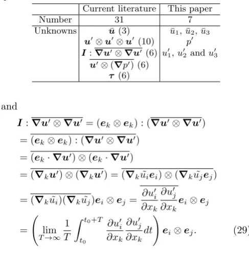
Current literature claims that Eq.27 has 31 independent unknowns. However, this research has a different opinion, and has proven that the Reynolds stress equation Eq. 27 only has 7 independent unknowns. Accoutring for all symmetries, these are listed in Table III below.
The above statement is proven by the following:
u0⊗u0⊗u0=u0iu0ju0kei⊗ej⊗ek
= lim
T→∞ 1 T
Z t0+T
t0
u0iu0ju0kdt !
ei⊗ej⊗ek, (28)
TABLE III: Number of unknowns in the Reynolds stress e-quation
Current literature This paper
Number 31 7
Unknowns u¯ (3) u1,¯ u2,¯ u3¯
u0⊗u0⊗u0 (10) p0
I:∇u0⊗∇u0 (6) u0 1, u
0 2 andu
0 3
u0⊗(∇p0) (6)
τ (6)
and
I:∇u0⊗∇u0= (e
k⊗ek) : (∇u0⊗∇u0) = (ek⊗ek) : (∇u0⊗∇u0)
= (ek·∇u0)⊗(ek·∇u0)
= (∇ku0)⊗(∇ku0) = (∇ku˜iei)⊗(∇ku˜jej)
= (∇ku˜i)(∇ku˜j)ei⊗ej = ∂u0i ∂xk
∂u0j
∂xk
ei⊗ej
= lim
T→∞ 1 T
Z t0+T
t0
∂u0 i ∂xk
∂u0j
∂xk dt
!
ei⊗ej. (29)
It is clear that the mean value ofu0iu0ju0k and ∂u0i ∂xk
∂u0
j ∂xk can be calculated by the velocity fluctuationsu01, u02 andu03. It means thatu01, u02and u03 are unknowns. Similarly,
u0⊗(∇p0) =u0 i
∂p0 ∂xj
ei⊗ej
= lim
T→∞ 1 T
Z t0+T
t0
u0i∂p 0
∂xj dt
!
ei⊗ej. (30)
The mean value of u0i∂x∂p0
j can be calculated by p 0 and u01, u02 andu03.
The same can also be done for the fourth order and for higher orders as in [32] and in textbooks. However, no other unknowns can be created by any order equation in respect of the Reynolds’ stress tensor.
VII. TRANSPORT EQUATION OF TURBULENCE KINETIC ENERGY
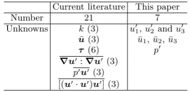
The contraction operation for indexiandjin Eq.27 re-sulted in the following transport equation for turbulence kinetic energyk
ρ¯u·∇k=τ :∇u¯
−µ∇u0:∇u0+µ∇2k
−∇·(p0u0)−1
2ρ∇·[(u
0·u0)u0], (31)
where the kinetic energy k(x) = −1 2τkk =
1 2u
0 ku
0 k = 1
2u0·u0 = limT→∞ 1 T
Rt0+T
t0 u
0·u0dt. The number of
TABLE IV: Number of unknowns in the kinetic energy equa-tion
Current literature This paper
Number 21 7
Unknowns k(3) u01, u 0 2 andu
0 3 ¯
u(3) u1,¯ u2,¯ u3¯
τ (6) p0
∇u0:∇u0 (3) p0u0 (3) [(u0·u0)u0] (3)
VIII. CONCLUSIONS
This article re-visited a fundamental problem in tur-bulence analysis, namely the number of independent un-knowns in the Reynolds’ stress tensor. The research s-tudy found that there are 3 independent unknowns in the Reynolds’ stress tensor, namely 3 components of velocity fluctuationsu01, u02andu03. This study has not only clar-ified the number of independent unknowns in the formu-lations of the Reynolds-averaged Navier-Stokes equation, but has also discovered that the number of independen-t unknowns is much less independen-than independen-tradiindependen-tionally found and thought.
In future, turbulence modelling should focus on the modelling of velocity fluctuations u01, u02, u03, instead of
on the Reynolds stressτij. An advantage of modelling the velocity fluctuationsu01, u02, u03 is that it reduces the six components ofτij into three ones, and from an ex-perimental perspective, the components of velocity fluc-tuations are easiest to measure than the Reynolds’ stress tensor.
It is important to point out that this study’s ideas and methodologies are also applicable to compressible turbu-lence Navier-Stokes equations, where the mass densityρ and the temperatureT must be taken into account, and their Reynolds decompositions,ρ= ¯ρ+ ˜ρandT = ¯T+ ˜T, should be introduced.
The present investigation can be considered as a re-naissance of Reynolds’ study in 1895, which might as-sist with understanding the well-known closure problem of turbulence, and the puzzle of the turbulence closure problem that has eluded scientists and mathematicians for centuries [63].
IX. ACKNOWLEDGEMENT
It is my great pleasure to have shared and discussed some thoughts of this paper with Michael Sun of Bishops Diocesan College, whose pure and direct scientific knowl-edge inspired me. This paper is dedicated to my beloved parents and family.
[1] Sydney Goldstein, Fluid Mechanics in the First Half of this Century, Annual Review of Fluid Mechanics, Vol. 1:1-29, 1969: http-s://doi.org/10.1146/annurev.fl.01.010169.000245 [2] https://en.wikipedia.org/wiki/Turbulence
[3] https://ideasranking.com/turbulence-one-of-the-great-unsolved-mysteries-of-physics-ted-ed.html
[4] D. Castelvecchi, Mysteries of turbulence unravelled, Na-ture, 548:382 (2017).
[5] K.R. Sreenivasan, On the scaling of the turbulence en-ergy dissipation rate. Physics of Fluids, 27,5:1048-1051 (1984).
[6] U. Frisch,Turbulence: The Legacy of A.N. Kolmogorov. Cambridge University Press,Cambridge (2008).
[7] G.K. Batchelor, The Theory of Homogeneous Turbu-lence. Cambridge University Press (1953).
[8] P. Bradshaw,An Introduction to Turbulence and Its Mea-surement. Pergamon Press, New York (1971).
[9] H. Tennekes and J.L. Lumley,A First Course in Turbu-lence. Cambridge: The MIT Press (1972).
[10] D.C. Lesilie,Developments in the Theory of Turbulence. Clarendon Press, Oxford (1973).
[11] A.A. Townsend,The Structure of Turbulent Shear Flow 2nd ed., Cambridge University Press, New York (1976). [12] M. Lesieur,Turbulence in Fluids. 2nd ed. Kluwer,
Dor-drecht (1990).
[13] D.C. Wilcox,Turbulence Modeling for CFD. D C W In-dustries (1993).
[14] S.B. Pope,Turbulent Flows. Cambridge University Press, Cambridge (2000).
[15] P.A. Davidson, Turbulence. Oxford University Press, Oxford (2004).
[16] B. Hof, Experimental Observation of Nonlinear Traveling Waves in Turbulent Pipe Flow. Science305, 1594 (2004). [17] G. Falkovich and K.R. Sreenivasan, Lessons from hydro-dynamic turbulence. Physics Today, 43-49 (April 2006). [18] P.A. Davison,et al. A Voyage Through Turbulence.
Cam-bridge: Cambridge University Press (2011).
[19] O. Reynolds, On the dynamical theory of incompress-ible viscous fluids and the determination of the criterion. Philos. Trans. R. Soc. 186:123-164(1895).
[20] Sir H. Lamb, Hydrodynamics, 6th edition, Cambdridge University Press, 1993.
[21] C. L. M. H. Navier, M´emoire sur les Lois du Mouvement des Fluides, M´em.de l’Acad.des Sciences, vi.389 (1822). [22] S.D. Poisson, M´emoire sur les ´Equations g´e´erales de
l’ ´Equilibre et du Mouvement des Corps solides ´elastiques et des Fluides, Journ.de l’ ´Ecole Plytechn.xiii. 1 (1829). [23] M. B. de Saint-Venant, Comptes Rendus, xvii.
1240(1843).
[24] G.G. Stokes, On the Theories of the Internal Friction of Fluids in Motion and of the Equilibrium and Motion of Elastic Solids. Trans. Cambridge Philos. Soc., 8, 287-319(1845).
[25] L. Prandtl, On fluid motions with very small friction (in German). Third International Mathematical Congress, Heidelberg. 484-491(1904).
[27] L. F. Richardson,Weather Prediction by Numerical Pro-cess. Cambridge University Press, 1922.
[28] L. Prandtl, Bericht uber die entstehung der turbulenz. Z. Angew. Math. Mech 5, 136(1925).
[29] James C. McWilliams, http://people.atmos.ucla.edu/jcm /turbulence course notes/.
[30] G. I. Taylor. Statistical theory of turbulence. Proc. R. Soc. Lond. A, 151:421-444, 1935.
[31] T. von Karman and L. Howarth On the statistical theory of isotropic turbulence. Proc. R. Soc. Lond. A, 164:192-215, 1938.
[32] P-Y. Chou, On velocity correlations and the solutions of the equations of turbulent fluctuation. Q. Appl. Math. 111(1):38-54(1945).
[33] P-Y. Chou and R.L. Chou, 50 years of turbulence re-search in China. Annu. Rev. Fluid Mech.27:1-15(1995). [34] R. H. Kraichnan, Hydrodynamic turbulence and the renormalization group. Phys.Rev. A, 25:3281-3289, 1982. [35] S.Y. Chen and P.-Y. Zhou, The application of quasi-similarity conditions in turbulence modeling theory. Journal of Hydrodynamics, 2(2) (1987)
[36] P. R. Spalart and S. R. Allmaras. A one-equation tur-bulence model for aerodynamics flows. La Recherche Aerospatiale, 1:5-21, 1994.
[37] P. Moin and K. Mahesh. Direct numerical simulation: a tool in turbulence research. Annu. Rev. Fluid Mech., 30:539-578, 1998.
[38] C.B. Lee and J.Z. Wu, Transition in wall-bounded flows. Applied Mechanics Reviews, 61(3), 030802 (2008). [39] I. Marusic, R. Mathis and N. Hutchins, Predictive
mod-el for wall-bounded turbulent Flow. Science 329, 193 (2010).
[40] A.J. Smits, B.J. McKeon and I. Marusic, High-Reynolds Number Wall Turbulence, Annu. Rev. Fluid Mech. 43, 353 (2011).
[41] B. Suri, J.R. Tithof, R.O. Grigoriev and M.F. Schatz, Forecasting Fluid Flows Using the Geometry of Turbu-lence. Phys. Rev. Lett.118, 114501 (2017).
[42] D. Castelvecchi, On the trial of turbulence. Nature, 548:382 (2017).
[43] S.P. Lloyd, The infinitesimal group of the Naviers-Stokes equations, Acta.Mech.,38:85-98(1981).
[44] L.D. Landau and E. M. Lifshitz, Mechanics (3rd ed.) (Butterworth-Heinemann, Oxford, 1976).
[45] A.N. Kolmogorov, The local structure of turbulence in incompressible viscous fluid for very large Reynold-s number. Dokl. Akad. Nauk SSSR, 30:299-303 (1941a) (reprinted in Proc.R.Soc.Lond.A, 434,9-13, 1991). [46] A.N. Kolmogorov, On degeneration (decay) of
isotrop-ic turbulence in an incompressible visous liquid. Dokl. Akad. Nauk SSSR,31:538-540 (1941b).
[47] A.N. Kolmogorov, Dissipation of energy in locally isotropic turbulence. Dokl.Akad. Nauk SSSR, 32 :16-18 (1941c).(reprinted in Proc.R.Soc.Lond. A, 434,15-17, 1991).
[48] N. Cao, S. Chen, and Z. S. She, Scalings and relative
s-calings in the Navier-Stokes turbulence. Phys. Rev. Lett., 76:3711-3714, 1996.
[49] Z.S. She and E. L´evˆeque, Universal scaling laws in fully developed turbulence. Phys. Rev. Lett.72,336(1994). [50] E.N. Lorenz, Deterministic non-periodic flow. J. Atmos
Sci.20:130-41(1963).
[51] R. Benzi, P. Paladin, G. Parisis and A. Vulpiani, On the multifractal nature of fully developed turbulence and chaotic systems. J. Phys. A: Math. Gen. 17 :3521-3531(1984).
[52] S.A. Orszag and G.S. Patterson, Numerical simulation of three-dimensional homogeneous isotropic turbulence. Phys. Rev. Lett.28,76(1972).
[53] H. Schlichting and K. Gersten,Boundary Layer Theory, 8th edition, Springer (2000).
[54] J. Baez and J.P. Muniain, Gauge Fields, Knots and Grav-ity, World Scientific (1994).
[55] B. Sun, The temporal scaling laws of compressible turbu-lence. Modern Physics Letters B.30,(23) 1650297 (2016). [56] B. Sun, Scaling laws of compressible turbulence. Appl.
Math. Mech.-Engl. Ed.38: 765(2017).
[57] B. Sun, Thirty years of turbulence study in China. Applied Mathematics and Mechanics (English Edition), 40(2), 193-214 (2019) (doi.org/10.1007/s10483-019-2427-9).
[58] B. Sun, A additive decomposition of ve-locity gradient, Physics of Fluids 31, 061702(2019)(doi:10.1063/1.5100872).
[59] B. Sun, On the Reynolds-averaged
Navier-Stokes equations. Preprints 2019 (doi:10.20944/preprints201907.0038.v1).
[60] B. Sun, On closure problem of incompress-ible turbulent flow. Preprints 2018, 2018070622 (doi:10.20944/preprints201807.0622.v2).
[61] B. Sun, An Intrinsic Formulation of Incompress-ible Navier-Stokes Turbulent Flow. Preprints 2018, 2018080071 (doi:10.20944/preprints201808.0071.v3). [62] B. Sun, A Novel Simplification of the
Reynolds-Chou-Navier-Stokes Turbulence Equations of In-compressible Flow. Preprints 2018, 2018070030 (doi:10.20944/preprints201807.0030.v1).
[63] Sun, B. Reynolds’ Turbulence Solution. Preprints 2019, 2019080138 (doi:10.20944/preprints201908.0138.v2). [64] B. Sun and Elaine S. Oran, New principle for
aerody-namic heating, National Science Review 00: 1-2, 2018 (doi:10.1093/nsr/nwy035).
[65] H. Hu, and B. Sun, New development in near-wall PIV measurements, Sci. China-Phys. Mech. Astron. 61, 094731 (2018)
[66] https://en.wikipedia.org/wiki/Dyadic tensor
[67] H. Blasius, Grenzschichten in Fljssigkeiten mit kleiner Reibung. Z. Math.Phys., 56 1-37(1908).