COVID-19 Outbreak Prediction with Machine
Learning
Sina F. Ardabili 1, Amir Mosavi 2,3,*, Pedram Ghamisi 4, Filip Ferdinand 2 , Annamaria R. Varkonyi-Koczy 2, Uwe Reuter 3, Timon Rabczuk 5, Peter M. Atkinson 6
1 Thuringian Institute of Sustainability and Climate Protection, 07743 Jena, Germany; [email protected] 2 Department of Mathematics and Informatics, J. Selye University, 94501 Komarno, Slovakia; [email protected] 3 Faculty of Civil Engineering, Technische Universität Dresden, 01069 Dresden, Germany.
4 Machine Learning Group, Exploration Division, Helmholtz Institute Freiberg for Resource Technology, Helmholtz-Zentrum Dresden-Rossendorf, Dresden, Germany; [email protected]
5 Institute of Structural Mechanics (ISM), Bauhaus-Universität Weimar, 99423 Weimar, Germany 6 Lancaster Environment Centre, Lancaster University, Lancaster LA1 4YQ, UK; [email protected] * Correspondence: [email protected]
Abstract: Several outbreak prediction models for COVID-19 are being used by officials around the world to make informed-decisions and enforce relevant control measures. Among the standard models for COVID-19 global pandemic prediction, simple epidemiological and statistical models have received more attention by authorities, and they are popular in the media. Due to a high level of uncertainty and lack of essential data, standard models have shown low accuracy for long-term prediction. Although the literature includes several attempts to address this issue, the essential generalization and robustness abilities of existing models needs to be improved. This paper presents a comparative analysis of machine learning and soft computing models to predict the COVID-19 outbreak. Among a wide range of machine learning models investigated, two models showed promising results (i.e., multi-layered perceptron, MLP, and adaptive network-based fuzzy inference system, ANFIS). Based on the results reported here, and due to the highly complex nature of the COVID-19 outbreak and variation in its behavior from nation-to-nation, this study suggests machine learning as an effective tool to model the outbreak.
Keywords: COVID-19; Coronavirus disease; Coronavirus; SARS-CoV-2; model; prediction; machine learning
1. Introduction
Access to accurate outbreak prediction models is essential to obtain insights into the likely spread and consequences of infectious diseases. Governments and other legislative bodies rely on insights from prediction models to suggest new policies and to assess the effectiveness of the enforced policies [1]. The novel Coronavirus disease (COVID-19) has been reported to infect more than 2 million people, with more than 132,000 confirmed deaths worldwide. The recent global COVID-19 pandemic has exhibited a nonlinear and complex nature [2]. In addition, the outbreak has differences with other recent outbreaks, which brings into question the ability of standard models to deliver accurate results [3]. Besides the numerous known and unknown variables involved in the spread, the complexity of population-wide behavior in various geopolitical areas and differences in containment strategies had dramatically increased model uncertainty [4]. Consequently, standard epidemiological models face new challenges to deliver more reliable results. To overcome this challenge, many novel models have emerged which introduce several assumptions to modeling (e.g., adding social distancing in the form of curfews, quarantines, etc.) [5-7].
To elaborate on the effectiveness of enforcing such assumptions understanding standard dynamic epidemiological (e.g., susceptible-infected-recovered, SIR) models is essential [8]. The modeling strategy is formed around the assumption of transmitting the infectious disease through contacts, considering three different classes of well-mixed populations; susceptible to infection (class
S), infected (class I), and the removed population (class R is devoted to those who have recovered, developed immunity, been isolated or passed away). It is further assumed that the class I transmits the infection to class S where the number of probable transmissions is proportional to the total number of contacts [9-11]. The number of individuals in the class S progresses as a time-series, often computed using a basic differential equation as follows:
𝑑𝑆
𝑑𝑡= −𝛼𝑆𝐼
(1)
where
𝐼
is the infected population, and 𝑆 is the susceptible population both as fractions. 𝛼represents the daily reproduction rate of the differential equation, regulating the number of susceptible infectious contacts. The value of 𝑆 in the time-series produced by the differential equation gradually declines. Initially, it is assumed that at the early stage of the outbreak 𝑆 ≈ 1 while the number of individuals in class I is negligible. Thus, the increment 𝑑𝐼𝑑𝑡 becomes linear and the class I eventually can be computed as follows:
𝑑𝐼
𝑑𝑡= 𝛼𝑆𝐼 − 𝛽𝐼 (2)
where 𝛽 regulates the daily rate of new infections by quantifying the number of infected individuals competent in the transmission. Furthermore, the class R, representing individuals excluded from the spread of infection, is computed as follows:
𝑑𝑅
𝑑𝑡 = 𝛽𝐼 (3)
Under the unconstrained conditions of the excluded group, Eq. 3, the outbreak exponential growth can be computed as follows:
𝐼 (𝑡) ≈ 𝐼0 𝑒𝑥𝑝{(𝛼 − 𝛽)} (4)
The outbreaks of a wide range of infectious diseases have been modeled using Eq. 4. However, for the COVID-19 outbreak prediction, due to the strict measures enforced by authorities, the susceptibility to infection has been manipulated dramatically. For example, in China, Italy, France, Hungary and Spain the SIR model cannot present promising results, as individuals committed voluntarily to quarantine and limited their social interaction. However, for countries where containment measures were delayed (e.g., United States) the model has shown relative accuracy [12]. Figure. 1 shows the inaccuracy of conventional models applied to the outbreak in Italy by comparing the actual number of confirmed infections and epidemiological model predictions1. The SEIR models through considering the significant incubation period during which individuals have been infected showed progress in improving the model accuracy for Varicella and Zika outbreak [13,14]. SEIR models assume that the incubation period is a random variable and similarly to the SIR model, there would be a disease-free-equilibrium [15,16]. It is worth mentioning that SEIR model will not work well where the parameters are non-stationary through time [17]. A key cause of non-stationarity is where the social mixing (which determines the contact network) changes through time. Social mixing determines the reproductive number 𝑅0 which is the number of susceptible individuals that an infected person will infect. Where 𝑅0 is less than 1 the epidemic will die out. Where it is greater than 1 it will spread. 𝑅0 for COVID-19 prior to lockdown was estimated as a massive 4 presenting a pandemic. It is expected that lockdown measures should bring 𝑅0 down to less than 1. the KEY reason why SEIR models are difficult to fit for COVID-19 is non-stationarity of mixing, caused by nudging (step-by-step) intervention measures.
COVID-19 in several countries demonstrates a high degree of uncertainty and complexity [26]. Thus, for epidemiological models to be able to deliver reliable results, they must be adapted to the local situation with an insight into susceptibility to infection [27]. This imposes a huge limit on the generalization ability and robustness of conventional models. Advancing accurate models with a great generalization ability to be scalable to model both the regional and global pandemic is, thus, essential [28].
A further drawback of conventional epidemiological models is the short lead-time. To evaluate the performance of the models, the median success of the outbreak prediction presents useful information. The median prediction factor can be calculated as follows:
𝑓 = 𝑃𝑟𝑒𝑑𝑖𝑐𝑡𝑖𝑜𝑛
𝑇𝑟𝑢𝑒 𝑣𝑎𝑙𝑢𝑒 (5)
As the lead-time increases, the accuracy of the model declines. For instance, for the COVID-19 outbreak in Italy, the accuracy of the model for more than 5-days-in-the-future reduces from 𝑓 = 1
for the first five days to 𝑓 = 0.86 for day 6 [12].
Figure 1. Italy’s COVID-19 outbreak: the actual number of confirmed infections vs. epidemiological model.
Due to the complexity and the large-scale nature of the problem in developing epidemiological models, machine learning (ML) has recently gained attention for building outbreak prediction models. ML approaches aim at developing models with higher generalization ability and greater prediction reliability for longer lead-times [29-33].
Table 1. Notable ML methods for outbreak prediction
Authors Journal Outbreak infection Machine learning
[39] Transboundary and
Emerging Diseases Swine fever Random Forest
[35] Geospatial Health Dengue fever Neural Network
[42] BMC Research Notes Influenza Random Forest
[41] Journal of Public
Health Medicine Dengue/Aedes Bayesian Network
[38] Informatica Dengue LogitBoost
[8] Global Ecology and
Biogeography H1N1 flu Neural Network
[34] Current Science Dengue Adopted multi-regression
and Naïve Bayes
[36] Environment
International Oyster norovirus Neural Network [37] Water Research Oyster norovirus Genetic programming
[43] Infectious Disease
Modelling Dengue
Classification and regression tree (CART)
The rest of this paper is organized as follows. Section two describes the methods and materials. The results are given in section three. Sections four and five present the discussion and the conclusions, respectively.
2. Materials and Methods
Data were collected from https://www.worldometers.info/coronavirus/country for five countries, including Italy, Germany, Iran, USA, and China on total cases over 30 days. Figure 2 presents the total case number (cumulative statistic) for the considered countries. Currently, to contain the outbreak, the governments have implemented various measures to reduce transmission through inhibiting people’s movements and social activities. Although for advancing the epidemiological models information on changes in social distancing is essential, for modeling with machine learning no assumption is required. As can be seen in Figure 2, the growth rate in China is greater than that for Italy, Iran, Germany and the USA in the early weeks of the disease.
The next step is to find the best model for the estimation of the time-series data. Logistic, Linear, Logarithmic, Quadratic, Cubic, Compound, Power and exponential equations (Table 2) are employed to develop the desired model.
Table 2. Models for mathematical forecasting
Model description Model name Equation number R=A/(1+exp(((4*µ)*(L-x)/A)+2)) Logistic (6)
R=Ax-B Linear (7)
R=A+ Blog(x) Logarithmic (8)
R=A+Bx+Cx2 Quadratic (9)
R=A+Bx+Cx2+Dx3 Cubic (10)
R=ABx Compound (11)
R=AxB Power (12)
R=AEXP(Bx) Exponential (13)
A, B, C, µ, and L are parameters (constants) that characterize the above-mentioned functions. These constants need to be estimated to develop an accurate estimation model. One of the goals of this study was to model time-series data based on the logistic microbial growth model. For this purpose, the modified equation of logistic regression was used to estimate and predict the prevalence (i.e., I/Population at a given time point) of disease as a function of time. Estimation of the parameters was performed using evolutionary algorithms like GA, particle swarm optimizer, and the grey wolf optimizer. These algorithms are discussed in the following.
Evolutionary algorithms
Evolutionary algorithms (EA) are powerful tools for solving optimization problems through intelligent methods. These algorithms are often inspired by natural processes to search for all possible answers as an optimization problem [46-48]. In the present study, the frequently used algorithms, (i.e., genetic algorithm (GA), particle swarm optimizer (PSO) and grey wolf optimizer (GWO)) are employed to estimate the parameters by solving a cost function.
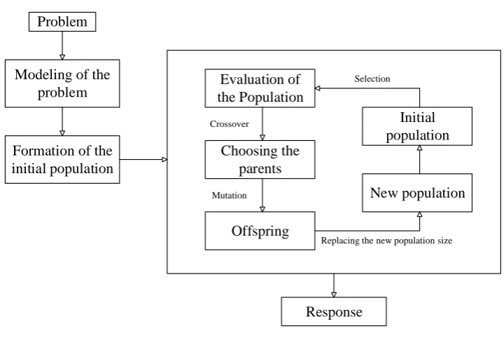
Genetic Algorithm (GA)
Problem
Modeling of the problem
Formation of the initial population
Evaluation of the Population
Choosing the parents
Offspring
New population Initial population
Response Crossover
Mutation
Replacing the new population size Selection
Figure 3. GA algorithm
In the present study, GA [59] was employed for estimation of the parameters of Eq. 6 to 13. The population number was selected to be 300 and the maximum generation (as iteration number) was determined to be 500 according to different trial and error processes to reduce the cost function value. The cost function was defined as the mean square error between the target and estimated values according to Eq. 14:
𝑀𝑆𝐸 = √(𝐸𝑠−𝑇)2
𝑁 (14)
where, Es refer to estimated values, T refers to the target values and N refers to the number of data.
Particle Swarm Optimization (PSO)
In 1995, Kennedy and Eberhart [60] introduced the PSO as an uncertain search method for optimization purposes. The algorithm was inspired by the mass movement of birds looking for food. A group of birds accidentally looked for food in a space. There is only one piece of food in the search space. Each solution in PSO is called a particle, which is equivalent to a bird in the bird's mass movement algorithm. Each particle has a value that is calculated by a competency function which increases as the particle in the search space approaches the target (food in the bird’s movement model). Each particle also has a velocity that guides the motion of the particle. Each particle continues to move in the problem space by tracking the optimal particles in the current state [60-62]. The PSO method is rooted in Reynolds' work, which is an early simulation of the social behavior of birds. The mass of particles in nature represents collective intelligence. Consider the collective movement of fish in water or birds during migration. All members move in perfect harmony with each other, hunt together if they are to be hunted, and escape from the clutches of a predator by moving another prey if they are to be preyed upon [63-65]. Particle properties in this algorithm include [65-67]:
• Each particle independently looks for the optimal point.
• Each particle moves at the same speed at each step.
• Each particle remembers its best position in the space.
• The particles work together to inform each other of the places they are looking for.
• Each particle is in contact with its neighboring particles.
• Every particle is aware of the particles that are in the neighborhood.
The PSO implementation steps can be summarized as: the first step establishes and evaluates the primary population. The second step determines the best personal memories and the best collective memories. The third step updates the speed and position. If the conditions for stopping are not met, the cycle will go to the second step.
The PSO algorithm is a population-based algorithm [68,69]. This property makes it less likely to be trapped in a local minimum. This algorithm operates according to possible rules, not definite rules. Therefore, PSO is a random optimization algorithm that can search for unspecified and complex areas. This makes PSO more flexible and durable than conventional methods. PSO deals with non-differential target functions because the PSO uses the information result (performance index or target function to guide the search in the problem area). The quality of the proposed route response does not depend on the initial population. Starting from anywhere in the search space, the algorithm ultimately converges on the optimal answer. PSO has great flexibility to control the balance between the local and overall search space. This unique PSO property overcomes the problem of improper convergence and increases the search capacity. All of these features make PSO different from the GA and other innovative algorithms [61,65,67].
In the present study, PSO was employed for estimation of the parameters of Eq. 6 to 13. The population number was selected to be 1000 and the iteration number was determined to be 500 according to different trial and error processes to reduce the cost function value. The cost function was defined as the mean square error between the target and estimated values according to Eq. 14.
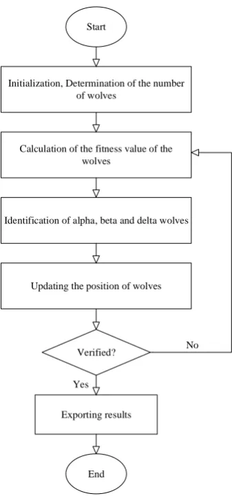
Grey Wolf Optimizer (GWO)
One recently developed smart optimization algorithm that has attracted the attention of many researchers is the grey wolf algorithm. Like most other intelligent algorithms, GWO is inspired by nature. The main idea of the grey wolf algorithm is based on the leadership hierarchy in wolf groups and how they hunt [70]. In general, there are four categories of wolves among the herd of grey wolves, alpha, beta, delta and omega. Alpha wolves are at the top of the herd's leadership pyramid, and the rest of the wolves take orders from the alpha group and follow them (usually there is only one wolf as an alpha wolf in each herd). Beta wolves are in the lower tier, but their superiority over Delta and omega wolves allows them to provide advice and help to alpha wolves. Beta wolves are responsible for regulating and orienting the herd based on alpha movement. Delta wolves, which are next in line for the power pyramid in the wolf herd, are usually made up of guards, elderly population, caregivers of damaged wolves, and so on. Omega wolves are also the weakest in the power hierarchy [70]. Eq. 15 to 18 are used to model the hunting tool:
𝐷⃗⃗ = |𝐶 , 𝑋⃗⃗⃗⃗ (𝑡) − 𝑋𝑝 ⃗⃗⃗ (𝑡)| (15)
𝑋 (𝑡 + 1) = 𝑋⃗⃗⃗⃗ (𝑡) − 𝐴 , 𝐷𝑝 ⃗⃗ (16)
𝐴 = 2𝑎 , 𝑟⃗⃗⃗ − 𝑎 1 (17)
𝐶 = 2𝑟⃗⃗⃗ 2 (18)
where t is represents repetition of the algorithm. 𝐴 and 𝐶 are vectors of the prey site and the 𝑋
Start
Initialization, Determination of the number of wolves
Calculation of the fitness value of the wolves
Identification of alpha, beta and delta wolves
Updating the position of wolves
Verified? No
Exporting results
End Yes
Figure 4. GWO algorithm
In the present study, GWO [70] was employed for estimation of the parameters of Eq.1 to 8. The population number was selected to be 500 and the iteration number was determined to be 1000 according to different trial and error processes to reduce the cost function value. The cost function was defined as the mean square error between the target and estimated values according to Eq. 14.
Machine learning (ML)
ML is regarded as a subset of AI. Using ML techniques, the computer learns to use patterns or “training samples” in data (processed information) to predict or make intelligent decisions without overt planning [71,72]. In other words, ML is the scientific study of algorithms and statistical models used by computer systems that use patterns and inference to perform tasks instead of using explicit instructions [73,74].
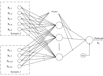
Time-series are data sequences collected over a period of time [75], which can be used as inputs to ML algorithms. This type of data reflects the changes that a phenomenon has undergone over time. Let Xt be a time-series vector, in which xt is the outbreak at time point t and T is the set of all equidistant time points. To train ML methods effectively, we defined two scenarios, listed in Table 3.
Table 3. Input and output variables for training ML methods by time-series data
Inputs Input number Output
Scenario 1 xt-1, xt-7, xt-14, and xt-21 Four inputs xt (outbreak)
As can be seen in Table 3, scenario 1 employs data for three weeks to predict the outbreak on day t and scenario 2 employs outbreak data for five days to predict the outbreak for day t. Both of these scenarios were employed for fitting the ML methods. In the present research, two frequently used ML methods, the multi-layered perceptron (MLP) and adaptive network-based fuzzy inference system (ANFIS) are employed for the prediction of the outbreak in the five countries.
Multi-layered perceptron (MLP)
ANN is an idea inspired by the biological nervous system, which processes information like the brain. The key element of this idea is the new structure of the information processing system [76-78]. The system is made up of several highly interconnected processing elements called neurons that work together to solve a problem [78,79]. ANNs, like humans, learn by example. The neural network is set up during a learning process to perform specific tasks, such as identifying patterns and categorizing information. In biological systems, learning is regulated by the synaptic connections between nerves. This method is also used in neural networks [80]. By processing experimental data, ANNs transfer knowledge or a law behind the data to the network structure, which is called learning. Basically, learning ability is the most important feature of such a smart system. A learning system is more flexible and easier to plan, so it can better respond to new issues and changes in processes [81].
In ANNs, with the help of programming knowledge, a data structure is designed that can act like a neuron. This data structure is called a node [82,83]. In this structure, the network between these nodes is trained by applying an educational algorithm to it. In this memory or neural network, the nodes have two active states (on or off) and one inactive state (off or 0), and each edge (synapse or connection between nodes) has a weight. Positive weights stimulate or activate the next inactive node, and negative weights inactivate or inhibit the next connected node (if active) [78,84]. In the ANN architecture, for the neural cell c, the input bp enters the cell from the previous cell p. wpc is the weight of the input bp with respect to cell c and ac is the sum of the multiplications of the inputs and their weights [85]:
𝑎
𝑐= ∑ 𝑤
𝑝𝑐𝑏
𝑝𝑐 (19)A non-linear function Өc is applied to ac. Accordingly, bc can be calculated as Eq. 20 [85]:
𝑏𝑐= 𝜃𝑐(𝑎𝑐) (20)
Similarly, wcn is the weight of the bcn which is the output of c to n. W is the collection of all the weights of the neural network in a set. For input x and output y, hw(x) is the output of the neural network. The main goal is to learn these weights for reducing the error values between y and hw(x). That is, the goal is to minimize the cost function Q(W), Eq. 21 [85]:
𝑄(𝑊) =1
2∑(𝑦𝑖− 𝑜𝑖)
2 𝑛
𝑖=1
(21)
x
t-1x
t-2x
t-3x
t-4x
t-5x
t-1x
t-7x
t-14x
t-21Scenario 2
Scenario 1
Weights
bias
Outbreak
x
tFigure 5. Architecture of MLP
Adaptive neuro fuzzy inference system (ANFIS)
An adaptive neuro fuzzy inference system is a type of ANN based on the Takagi-Sugeno fuzzy system [86]. This approach was developed in the early 1990s. Since this system integrates the concepts of neural networks and fuzzy logic, it can take advantage of both capabilities in a unified framework. This technique is one of the most frequently used and robust hybrid ML techniques. It is consistent with a set of fuzzy if-then rules that can be learned to approximate nonlinear functions [87,88]. Hence, ANFIS was proposed as a universal estimator. An important element of fuzzy systems is the fuzzy partition of the input space [89,90]. For input k, the fuzzy rules in the input space make a k faces fuzzy cube. Achieving a flexible partition for nonlinear inversion is non-trivial. The idea of this model is to build a neural network whose outputs are a degree of the input that belongs to each class [91-93]. The membership functions (MFs) of this model can be nonlinear, multidimensional and, thus, different to conventional fuzzy systems [94-96]. In ANFIS, neural networks are used to increase the efficiency of fuzzy systems. The method used to design neural networks is to employ fuzzy systems or fuzzy-based structures. This model is a kind of division and conquest method. Instead of using one neural network for all the input and output data, several networks are created in this model:
• A fuzzy separator to cluster input-output data within multiple classes.
• A neural network for each class.
Inputs
Input MFs
Rules
Output MF
Output
Input 1
Input 2
Input n
Output
Figure 6. ANFIS architecture
In the present study, ANFIS is developed to tackle two scenarios described in table 3. Each input included by two MFs with the Tri. shape; Trap. shape and Gauss. shape MFs. The output MF type was selected to be linear with a hybrid optimizer type.
Evaluation criteria
Evaluation was conducted using the root mean square error (RMSE) and correlation coefficient. These statistics compare the target and output values and calculate a score as an index for the performance and accuracy of the developed methods [87,97]. Table 4 presents the evaluation criteria equations.
Table 4. Model Evaluation metrics
Accuracy and Performance Index
Correlation coefficient= 𝑁 ∑ (𝐴𝑃)−∑ (𝐴)∑ (𝑃)
√[𝑁 ∑ 𝐴2−(∑ 𝐴) 2][𝑁 ∑ 𝑃2−(∑ 𝐴𝑃) 2] (22)
RMSE= √1
𝑁∑ (𝐴 −𝑃)
2 (23)
Where, N is the number of data, P and A are, respectively, the predicted (output) and desired (target) values.
3. Results
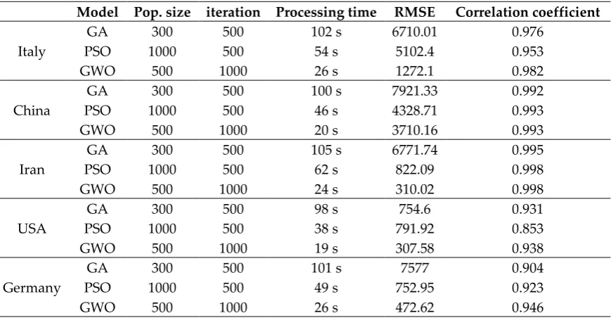
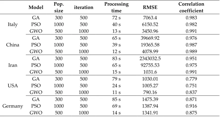
Tables 5 to 12 present the results of the accuracy statistics for the logistic, linear, logarithmic, quadratic, cubic, compound, power and exponential equations, respectively. The coefficients of each equation were calculated by the three ML optimizers; GA, PSO and GWO. The table contains country name, model name, population size, number of iterations, processing time, RMSE and correlation coefficient.
Table 5. Accuracy statistics for the logistic model
Country Model Pop. size iteration Processing time RMSE Correlation coefficient
Italy GA 300 500 82 s 1028.98 0.996
GWO 500 1000 14 s 187.15 0.999
China
GA 300 500 79 s 42160.4 0.982
PSO 1000 500 35 s 2524.44 0.994
GWO 500 1000 13 s 2270.58 0.995
Iran
GA 300 500 81 s 1267.04 0.992
PSO 1000 500 36 s 628.62 0.997
GWO 500 1000 13 s 392.88 0.996
USA
GA 300 500 82 s 1028.98 0.999
PSO 1000 500 38 s 350.33 0.999
GWO 500 1000 15 s 22.35 0.999
Germany
GA 300 500 86 s 5339.5 0.983
PSO 1000 500 39 s 555.32 0.997
GWO 500 1000 16 s 55.54 0.999
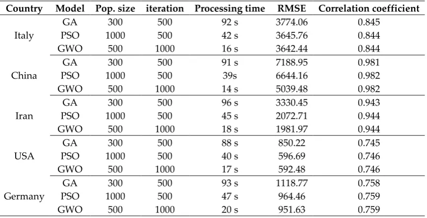
Table 6. Accuracy statistics for the linear model
Country Model Pop. size iteration Processing time RMSE Correlation coefficient
Italy
GA 300 500 92 s 3774.06 0.845
PSO 1000 500 42 s 3645.76 0.844
GWO 500 1000 16 s 3642.44 0.844
China
GA 300 500 91 s 7188.95 0.981
PSO 1000 500 39s 6644.16 0.982
GWO 500 1000 14 s 5039.48 0.982
Iran
GA 300 500 96 s 3330.45 0.943
PSO 1000 500 45 s 2072.71 0.944
GWO 500 1000 18 s 1981.97 0.944
USA
GA 300 500 88 s 850.22 0.745
PSO 1000 500 40 s 596.69 0.746
GWO 500 1000 17 s 592.48 0.746
Germany
GA 300 500 93 s 1118.77 0.758
PSO 1000 500 47 s 964.46 0.759
GWO 500 1000 20 s 951.63 0.759
Table 7. Accuracy statistics for the logarithmic model
Model Pop. size iteration Processing
time RMSE Correlation coefficient
Italy
GA 300 500 98 s 8325.33 0.634
PSO 1000 500 51 s 8818.2 0.634
GWO 500 1000 20 s 9296.59 0.634
China
GA 300 500 96 s 40828.2 0.847
PSO 1000 500 42 s 43835.37 0.847
GWO 500 1000 17 s 42714.93 0.847
Iran
GA 300 500 102 s 4929.97 0.757
PSO 1000 500 59 s 8775.56 0.757
GWO 500 1000 22 s 8995.52 0.756
USA
GA 300 500 94 s 889.15 0.538
PSO 1000 500 37 s 1130.33 0.538
GWO 500 1000 15 s 1135.12 0.538
Germa ny
PSO 1000 500 45 s 1966.81 0.548
GWO 500 1000 21 s 1878.67 0.548
Table 8. Accuracy statistics for the quadratic model
Model Pop. size iteration Processing time RMSE Correlation coefficient
Italy
GA 300 500 102 s 6710.01 0.976
PSO 1000 500 54 s 5102.4 0.953
GWO 500 1000 26 s 1272.1 0.982
China
GA 300 500 100 s 7921.33 0.992
PSO 1000 500 46 s 4328.71 0.993
GWO 500 1000 20 s 3710.16 0.993
Iran
GA 300 500 105 s 6771.74 0.995
PSO 1000 500 62 s 822.09 0.998
GWO 500 1000 24 s 310.02 0.998
USA
GA 300 500 98 s 754.6 0.931
PSO 1000 500 38 s 791.92 0.853
GWO 500 1000 19 s 307.58 0.938
Germany
GA 300 500 101 s 7577 0.904
PSO 1000 500 49 s 752.95 0.923
GWO 500 1000 26 s 472.62 0.946
Table 9. Accuracy statistics for the cubic model
Model Pop. size iteration Processing time RMSE Correlation coefficient
Italy
GA 300 500 112 s 7973.11 0.993
PSO 1000 500 61 s 4827.08 0.996
GWO 500 1000 34 s 324.33 0.998
China
GA 300 500 113 s 15697.84 0.971
PSO 1000 500 59 s 3611.15 0.995
GWO 500 1000 34 s 2429.45 0.995
Iran
GA 300 500 120 s 5852.66 0.995
PSO 1000 500 88 s 3809.76 0.997
GWO 500 1000 39 s 250.2 0.999
USA
GA 300 500 110 s 37766.56 0.875
PSO 1000 500 49 s 678.36 0.979
GWO 500 1000 25 s 118.24 0.991
Germany
GA 300 500 116 s 1709.06 0.744
PSO 1000 500 59 s 1812.78 0.967
GWO 500 1000 29 s 196.8 0.99
Table 10. Accuracy statistics for the compound model
Model Pop.
size iteration
Processing
time RMSE
Correlation coefficient
Italy
GA 300 500 92 s 8347.51 0.912
PSO 1000 500 53 s 195705.52 0.918
China
GA 300 500 90 s 41544.05 0.986
PSO 1000 500 48 s 40195.9 0.988
GWO 500 1000 23 s 24987.34 0.895
Iran
GA 300 500 99 s 1487501.93 0.782
PSO 1000 500 81 s 8216.81 0.986
GWO 500 1000 26 s 13635.01 0.864
USA
GA 300 500 96 s 655.62 0.994
PSO 1000 500 32 s 1026.03 0.827
GWO 500 1000 16 s 364.87 0.988
Germany
GA 300 500 98 s 15333537.7 0.93
PSO 1000 500 72 s 1557.23 0.976
GWO 500 1000 20 s 431.97 0.998
Table 11. Accuracy statistics for the power model
Model Pop.
size iteration
Processing
time RMSE
Correlation coefficient
Italy
GA 300 500 72 s 7063.4 0.983
PSO 1000 500 40 s 6150.52 0.982
GWO 500 1000 13 s 3450.96 0.991
China
GA 300 500 65 s 39669.92 0.976
PSO 1000 500 39 s 19365.58 0.987
GWO 500 1000 12 s 4078.99 0.989
Iran
GA 300 500 83 s 2343032.5 0.951
PSO 1000 500 65 s 92755.53 0.975
GWO 500 1000 15 s 1031.6 0.991
USA
GA 300 500 79 s 1030.01 0.779
PSO 1000 500 24 s 1005.27 0.751
GWO 500 1000 11 s 790.16 0.837
Germany
GA 300 500 85 s 1475.39 0.871
PSO 1000 500 69 s 1387.94 0.916
GWO 500 1000 14 s 1341.91 0.875
Table 12. Accuracy statistics for the exponential model
Model Pop.
size iteration
Processing
time RMSE
Correlation coefficient
Italy
GA 300 500 79 s 8163.1 0.995
PSO 1000 500 48 s 52075925.37 0.839
GWO 500 1000 18 s 12585.79 0.951
China
GA 300 500 71 s 68991.73 0.866
PSO 1000 500 45 s 80104.27 0.865
GWO 500 1000 17 s 24987.34 0.895
Iran
GA 300 500 89 s 1436025.84 0.767
PSO 1000 500 70 s 3745673.26 0.744
GWO 500 1000 21 s 13635.01 0.864
USA GA 300 500 84 s 457051.4 0.974
GWO 500 1000 15 s 364.87 0.988
Germany
GA 300 500 87 s 8176.54 0.981
PSO 1000 500 74 s 3278.55 0.998
GWO 500 1000 19 s 431.97 0.998
According to Tables 5 to 12, GWO provided the highest accuracy (smallest RMSE and largest correlation coefficient) and smallest processing time compared to PSO and GA for fitting the logistic, linear, logarithmic, quadratic, cubic, power, compound, and exponential-based equations for all five countries. It can be suggested that GWO is a sustainable optimizer due to its acceptable processing time compared with PSO and GA. Therefore, GWO was selected as the best optimizer by providing the highest accuracy values compared with PSO and GA. In general, it can be claimed that GWO, by suggesting the best parameter values for the functions presented in Table 2, increases outbreak prediction accuracy for COVID-19 in comparison with PSO and GA. Therefore, the functions derived by GWO were selected as the best predictors for this research.
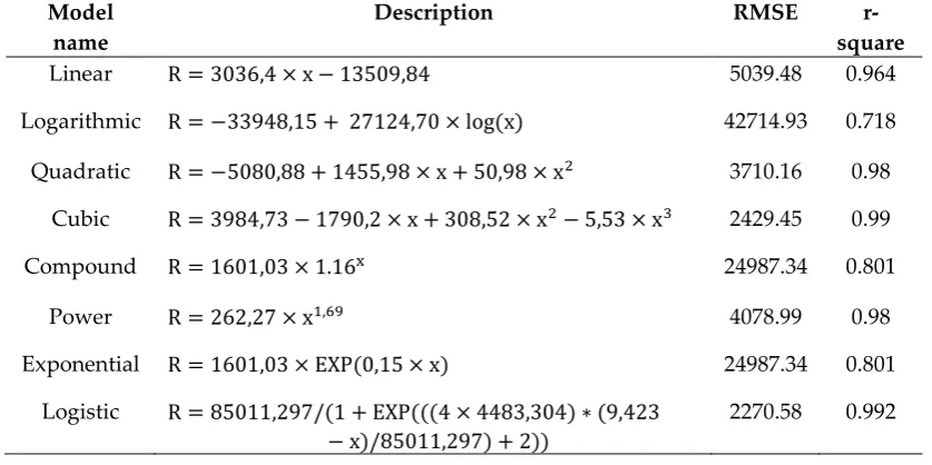
Tables 13 to 17 present the description and coefficients of the linear, logarithmic, quadratic, cubic, compound, power, exponential and logistic equations estimated by GWO. Tables 13 to 17 also present the RMSE and r-square values for each equation fitted to data for China, Italy, Iran, Germany and USA, respectively.
Table 13. Model description for China fitted by GWO
Model name
Description RMSE
r-square
Linear R = 3036,4 × x − 13509,84 5039.48 0.964
Logarithmic R = −33948,15 + 27124,70 × log(x) 42714.93 0.718
Quadratic R = −5080,88 + 1455,98 × x + 50,98 × x2 3710.16 0.98
Cubic R = 3984,73 − 1790,2 × x + 308,52 × x2− 5,53 × x3 2429.45 0.99
Compound R = 1601,03 × 1.16x 24987.34 0.801
Power R = 262,27 × x1,69 4078.99 0.98
Exponential R = 1601,03 × EXP(0,15 × x) 24987.34 0.801
Logistic R = 85011,297/(1 + EXP(((4 × 4483,304) ∗ (9,423 − x)/85011,297) + 2))
2270.58 0.992
Table 14. Model description for Italy fitted by GWO
Model name Description RMSE
r-square
Linear R = 663,71 × x − 5437,25 3642.44 0.713
Logarithmic R = −7997,93 + 5162,83 × log(x) 9296.59 0.402
Cubic R = −978,55 + 506,05 × B2 − 61,95 × x2
+ 2,42 × x3
324.33 0.997
Compound R = 2,78 × 1,406x 12585.79 0.904
Power R = 0,096 × x3,476 3450.96 0.984
Exponential R = 2,786 × EXP(0,341 × x) 12585.79 0.904
Logistic R = 70731,084/(1
+ EXP(((4 × 3962,88) × (23,88 − x)/70731,08) + 2))
187.15 0.999
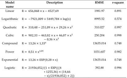
Table 15. Model description for Iran fitted by GWO
Model name
Description RMSE r-square
Linear R = 656,068 × x − 4527,69 1981.97 0.891
Logarithmic R = −7921,009 + 5449,784 × log(x) 8995.52 0.574
Quadratic R = 310,48 − 251,09 × x + 29,26 × x2 310.027 0.997
Cubic R = 902,33 − 463,02 × x + 46,07 × x2
− 0,36 × x3
250.204 0.998
Compound R = 13,26 × 1,33x 13635.014 0.748
Power R = 0,51 × x3,09 1031.607 0.982
Exponential R = 13,26 × EXP(0,28 × x) 13635.014 0.748
Logistic R = 21936,052/(1 + EXP(((4 ∗ 1255,36) × (14,66 − x)/21936,052) + 2))
392.88 0.996
Table 16. Model description for Germany fitted by GWO
Model name
Description RMSE
r-square
Linear R = 128,421 × x − 1130,294 951.635 0.577
Logarithmic R = −1528,684 + 959,941 × log(x) 1878.672 0.3
Quadratic R = 911,113 − 254,342 × x + 12,347 × x2 472.624 0.895
Cubic R = −478,087 + 243,097 × x − 27,118 × x2+ 0,848 × x3 196.809 0.981
Power R = 0,937x2,021 1341.911 0.766
Exponential R = 3,821 × EXP(0,233 × x) 431.975 0.996
Logistic R = 55179,669/(1 + EXP(((4 × 3740,457) × (30,49 − x)/55179,669) + 2))
55.546 0.998
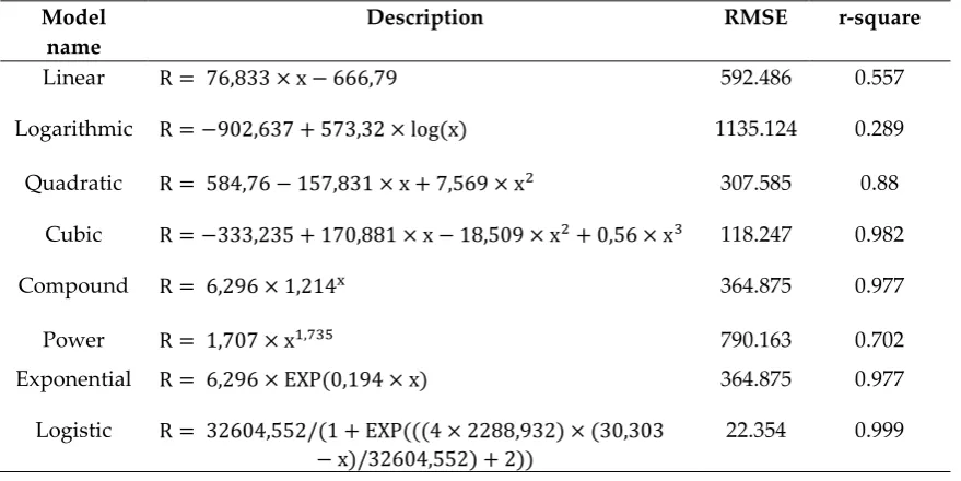
Table 17. Model description for USA fitted by GWO
Model name
Description RMSE r-square
Linear R = 76,833 × x − 666,79 592.486 0.557
Logarithmic R = −902,637 + 573,32 × log(x) 1135.124 0.289
Quadratic R = 584,76 − 157,831 × x + 7,569 × x2 307.585 0.88
Cubic R = −333,235 + 170,881 × x − 18,509 × x2+ 0,56 × x3 118.247 0.982
Compound R = 6,296 × 1,214x 364.875 0.977
Power R = 1,707 × x1,735 790.163 0.702
Exponential R = 6,296 × EXP(0,194 × x) 364.875 0.977
Logistic R = 32604,552/(1 + EXP(((4 × 2288,932) × (30,303 − x)/32604,552) + 2))
22.354 0.999
Figure 7. Fitness graph for China fitted by GWO
Figure 9. Set of models for Iran fitted by GWO
Figure 11. Set of models for USA fitted by GWO
Figures 7 to 11 illustrate the fit of the models investigated in this paper. The best fit for the prediction of COVID-19 cases was achieved for the logistic model followed by cubic and quadratic models for China (Figure 7), logistic followed by cubic models for Italy (Figure 8), cubic followed by logistic and quadratic models for Iran (Figure 9), the logistic model for Germany (Figure 10), and logistic model for the USA (Figure 11).
Machine learning results
This section presents the results for the training stage of ML methods. MLP and ANFIS were employed as single and hybrid ML methods, respectively. ML methods were trained using two datasets related to scenario 1 and scenario 2. Table 14 presents the results of the training phase.
Table 18. Results for the training phase of the ML methods
Scenario 1 Scenario2
MLP ANFIS MLP ANFIS
No. of
neurons r RMSE MF
type r RMSE
No. of
neurons r RMSE MF
type r RMSE
Italy
8 0.999 190.81 Tri. 0.999 189.76 8 0.999 199.52 Tri. 0.999 188.55
12 0.999 194.84 Trap. 0
.841 3743.63 12 0.999 195.79 Trap. 0.876 3276
16 0.999 188.18 Gauss 0.998 320.93 16 0.999 195.2 Gauss 0.999 206.66
Average 0.999 191.27 0.946 1418.1 Average 0.999 196.83 0.958 1223.73
12 0.996 2259.95 Trap. 0.987 4231.05 12 0.996 2285.73 Trap. 0.989 3835.34
16 0.995 2407.16 Gauss 0.996 2358.3 16 0.996 2260.05 Gauss 0.996 2272.58
Average 0.995 2318.22 0.993 2960.81 Average 0.996 2270.57 0.993 2793.35
Iran
8 0.998 392.17 Tri. 0.998 395.33 8 0.998 404.21 Tri. 0.998 394.04
12 0.998 391.04 Trap. 0.977 1282.33 12 0.998 392.77 Trap. 0.986 994
16 0.998 392.19 Gauss 0.998 396.51 16 0.998 395.43 Gauss 0.998 391.96
Average 0.998 391.8 0.991 391.39 Average 0.998 397.47 0.994 593.33
Germany
8 0.999 55.6 Tri. 0.999 56.25 8 0.999 55.58 Tri. 0.999 55.63
12 0.999 55.38 Trap. 0.12 1658.7 12 0.999 55.56 Trap. 0.13 1537.26
16 0.999 55.58 Gauss 0.998 154.99 16 0.999 55.56 Gauss 0.999 62.91
Average 0.999 55.52 0.705 623.31 Average 0.999 55.56 0.709 551.93
USA
8 0.999 21.65 Tri. 0.999 21.75 8 0.999 22.31 Tri. 0.999 22.52
12 0.999 22.36 Trap. 0.22 861.08 12 0.999 22.3 Trap. 0.2 935.41
16 0.999 22.31 Gauss 0.998 86.32 16 0.999 22.4 Gauss 0.999 25.03
Average 0.999 22.1 0.739 323.05 Average 0.999 22.33 0.739 327.65
According to Table 18, the dataset related to scenarios 1 and 2 have different performance values. Accordingly, for Italy, the MLP with 16 neurons provided the highest accuracy for scenario 1 and ANFIS with tri. MF provided the highest accuracy for scenario 2. By considering the average values of the RMSE and correlation coefficient, it can be concluded that scenario 1 is more suitable for modeling outbreak cases in Italy, as it provides a higher accuracy (the smallest RMSE and the largest correlation coefficient) than scenario 2.
For the dataset related to China, for both scenarios, MLP with 12 and 16 neurons, respectively for scenarios 1 and 2, provided the highest accuracy compared with the ANFIS model. By considering the average values of RMSE and correlation coefficient, it can be concluded that scenario 2 with a larger average correlation coefficient and smaller average RMSE than scenario 1 is more suitable for modeling the outbreak in China.
For the dataset of Iran, MLP with 12 neurons in the hidden layer for scenario 1 and ANFIS with Gaussian MF type for scenario 2 provided the best performance for the prediction of the outbreak. By considering the average values of the RMSE and correlation coefficient, it can be concluded that scenario 1 provided better performance than scenario 2. Also, in general, the MLP has higher prediction accuracy compared with the ANFIS method.
In Germany, MLP with 12 neurons in its hidden layer provided the highest accuracy (smallest RMSE and largest correlation coefficient). By considering the average values of the RMSE and correlation coefficient, it can be concluded that scenario 1 is more suitable for the prediction of the outbreak in Germany than scenario 2.
In the USA, the MLP with 8 and 12 neurons, respectively, for scenarios 1 and 2, provided higher accuracy (the smallest RMSE and the largest correlation coefficient values) than the ANFIS model. By considering the average values of the RMSE and correlation coefficient values, it can be concluded that scenario 1 is more suitable than scenario 2, and MLP is more suitable than ANFIS for outbreak prediction.
Figure 12. Set of models for Italy fitted by ML methods
Figure 14. Set of models for Iran fitted by ML methods
Figure 16. Set of models for USA fitted by ML methods
Comparing the fitted models
This section presents a comparison of the accuracy and performance of the selected models for the prediction of 30 days’ outbreak. Figure 17 to 21 shows the deviation from the target values for the selected models.
Figure 18. Deviation from target value for models related to China
Figure 19. Deviation from target value for models related to Iran
Figure 21. Deviation from target value for models related to USA
As is clear from Figure 17 to 21, the smallest deviation from the target values is related to the MLP for scenario 1 followed by MLP for scenario 2. This indicates the highest performance of the MLP method for the prediction of the outbreak.
Figures 22 to 26 present the outbreak prediction for 75 days and Tables 19 to 23 present the outbreak prediction for 150 days.
Table 19. The outbreak prediction for Italy through 150 days
Logistic by GWO
Linear by GWO
Logarithmic by GWO
Quadratic by GWO
Power by
GWO MLP ANFIS
Day
20th 3794.045 7837.054 -1280.93 5047.906 3225.523 3792.734 3796.738 Day
40th 58966.55 21111.37 273.235 47914.4 35898.08 58966.74 58964.96 Day
60th 70571.86 34385.68 1182.365 131597.7 146966.2 70571.66 70572.12 Day
80th 70729.28 47659.99 1827.402 256097.8 399523.4 70729.27 70729.15 Day
100th 70731.06 60934.31 2327.733 421414.7 867822 70731.09 70730.93 Day
120th 70731.08 74208.62 2736.532 627548.4 1635643 70731.14 70730.87 Day
140th 70731.08 87482.94 3082.167 874498.9 2795218 70731.19 70730.79 Day
150th 70731.08 94120.09 3236.862 1013280 3552851 70731.21 70730.75
Figure 23. The outbreak prediction for China through 75 days
Table 20. The outbreak prediction for China through 150 days
Logistic by GWO
Linear by GWO
Logarithmic by GWO
Quadratic by GWO
Power by
Day
20th 47397.6 47218.47 1341.899 44431.48 41916.55 47397.6 47360.98
Day
40th 84030.16 107946.8 9507.249 134729.1 135599.1 84030.17 84030.39
Day
60th 84996.7 168675.1 14283.67 265812 269471.3 84996.7 84996.67
Day
80th 85011.08 229403.4 17672.6 437680.2 438660.2 85011.08 85011.05
Day
100th 85011.29 290131.7 20301.26 650333.6 640132.8 85011.3 85011.22
Day
120th 85011.3 350860 22449.02 903772.3 871733.6 85011.34 85011.13
Day
140th 85011.3 411588.3 24264.94 1197996 1131815 85011.38 85011.05
Day
150th 85011.3 441952.5 25077.68 1360403 1272113 85011.41 85011.01
Figure 24. The outbreak prediction for Iran through 75 days
Table 21. The outbreak prediction for Iran through 150 days
Logistic by GWO Linear by
GWO
Logarithmic by GWO
Quadratic by GWO
Power by
GWO MLP ANFIS
Day 20th 6898.344 8593.676 -830.677 6993.955 5494.377 6902.315 6875.585
Day 40th 21455.58 21715.05 809.8719 37087.98 47060.48 21457.4 21456.65
Day 80th 21936 47957.8 2450.42 167507.7 403082.8 21935.1 21935.54
Day 100th 21936.05 61079.18 2978.559 267833.4 804764.4 21935.11 21935.6
Day 120th 21936.05 74200.55 3410.08 391569.6 1415829 21935.12 21935.63
Day 140th 21936.05 87321.93 3774.925 538716.4 2282679 21935.13 21935.65
Day 150th 21936.05 93882.61 3938.219 621068.7 2826737 21935.13 21935.67
Figure 25. The outbreak prediction for Germany through 75 days
Table 22. The outbreak prediction for Germany through 150 days
Logistic by GWO
Linear by GWO
Logarithmic by GWO
Quadratic by GWO
Power by GWO
MLP ANFIS
Day
20th 431.027 1438.128 -279.772 763.1467 400.0548 432.8991 431.8119 Day
40th 35356.27 4006.551 9.199328 10492.96 1624.405 35355.14 35355.72 Day
60th 55043.44 6574.974 178.2366 30100.56 3687.126 55036.14 55044.03 Day
80th 55179.07 9143.397 298.1705 59585.93 6595.829 55179.05 55178.88
Day
100th 55179.67 11711.82 391.1984 98949.09 10355.87 55179.9 55179.47 Day
Day
140th 55179.67 16848.66 531.4728 207308.7 20445.86 55179.94 55179.37 Day
150th 55179.67 18132.88 560.2357 240572.3 23506.09 55179.96 55179.35
Figure 26. The outbreak prediction for the USA through 75 days
Table 23. The outbreak prediction for the USA for 150 days
Logistic by GWO
Linear by GWO
Logarithmic by GWO
Quadratic by GWO
Power by GWO
MLP ANFIS
Day
20th 242.6091 869.8855 -156.73 456.0663 309.616 244.0038 243.6504
Day
40th 21951.15 2406.562 15.85698 6383.264 1031.324 21942.25 21948.25 Day
60th 32547.08 3943.238 116.8138 18366.35 2084.876 32552.6 32548.47 Day
80th 32604.34 5479.914 188.4437 36405.33 3435.319 32606.19 32604.47 Day
100th 32604.55 7016.591 244.0043 60500.21 5060.548 32606.63 32604.72
Day
120th 32604.55 8553.267 289.4005 90650.97 6944.676 32606.7 32604.76 Day
140th 32604.55 10089.94 327.7825 126857.6 9075.446 32606.78 32604.8 Day
4. Discussion
The parameters of several simple mathematical models (i.e., logistic, linear, logarithmic, quadratic, cubic, compound, power and exponential) were fitted using GA, PSO, and GWO. The logistic model outperformed other methods and showed promising results on training for 30 days. Extrapolation of the prediction beyond the original observation range of 30-days should not be expected to be realistic considering the new statistics. The fitted models generally showed low accuracy and also weak generalization ability for the five countries. Although the prediction for China was promising, the model was insufficient for extrapolation, as expected. In turn, the logistic GWO outperformed the PSO and GA and the computational cost for GWO was reported as satisfactory. Consequently, for further assessment of the ML models, the logistic model fitted with GWO was used for comparative analysis.
In the next step, for introducing the machine learning methods for time-series prediction, two scenarios were proposed. Scenario 1 considered four data samples from the progress of the infection from previous days, as reported in table 3. The sampling for data processing was done weekly for scenario 1. However, scenario 2 was devoted to daily sampling for all previous consecutive days. Providing these two scenarios expanded the scope of this study. Training and test results for the two machine learning models (MLP and ANFIS) were considered for the two scenarios. A detailed investigation was also carried out to explore the most suitable number of neurons. For the MLP, the performances of using 8, 12 and 16 neurons were analyzed throughout the study. For the ANFIS, the membership function (MF) types of Tri, Trap, and Gauss were analyzed throughout the study. The five counties of Italy, China, Iran, Germany, and USA were considered. The performance of both ML models for these countries varied amongst the two different scenarios. Given the observed results, it is not possible to select the most suitable scenario. Therefore, both daily and weekly sampling can be used in machine learning modeling. Comparison between analytical and machine learning models using the deviation from the target value (figures 17 to 21) indicated that the MLP in both scenarios delivered the most accurate results. Extrapolation for long-term prediction of up to 150 days using the ML models was tested. The actual prediction of MLP and ANFIS for the five countries was reported which showed the progression of the outbreak.
5. Conclusions
The global pandemic of the severe acute respiratory syndrome Coronavirus 2 (SARS-CoV-2) has become the primary national security issue of many nations. Advancement of accurate prediction models for the outbreak is essential to provide insights into the spread and consequences of this infectious disease. Due to the high level of uncertainty and lack of crucial data, standard epidemiological models have shown low accuracy for long-term prediction. This paper presents a comparative analysis of ML and soft computing models to predict the COVID-19 outbreak. The results of two ML models (MLP and ANFIS) reported a high generalization ability for long-term prediction. With respect to the results reported in this paper and due to the highly complex nature of the COVID-19 outbreak and differences from nation-to-nation, this study suggests ML as an effective tool to model the outbreak.
For the advancement of higher performance models for long-term prediction, future research should be devoted to comparative studies on various ML models for individual countries. Due to the fundamental differences between the outbreak in various countries, advancement of global models with generalization ability would not be feasible. As observed and reported in many studies, it is unlikely that an individual outbreak will be replicated elsewhere [1].
Although the most difficult prediction is to estimate the maximum number of infected patients, estimation of the n(deaths) / n(infecteds) is also essential. The mortality rate is particularly important to accurately estimate the number of patients and the required beds in intensive care units. For future research, modeling the mortality rate would be of the utmost importance for nations to plan for new facilities.
Nomenclatures
Multi-layered perceptron MLP Grey wolf optimization GWO
Adaptive network-based fuzzy inference system ANFIS Mean square error MSE Susceptible-infected-recovered SIR Root mean square error RMSE
Call data record CDR Artificial intelligence AI
Classification and regression tree CART Artificial neural network ANN
Evolutionary algorithms EA Triangular Tri.
Genetic algorithm GA Gaussian Gauss.
Particle swarm optimization PSO Trapezoidal Trap.
Membership function MF Machine learning ML
Conflicts of Interest: The authors declare no conflict of interest.
References
1. Remuzzi, A.; Remuzzi, G. COVID-19 and Italy: what next? Lancet 2020.
2. Ivanov, D. Predicting the impacts of epidemic outbreaks on global supply chains: A simulation-based analysis on the coronavirus outbreak (COVID-19/SARS-CoV-2) case. Transp. Res. Part E Logist. Transp. Rev. 2020, 136, doi:10.1016/j.tre.2020.101922.
3. Koolhof, I.S.; Gibney, K.B.; Bettiol, S.; Charleston, M.; Wiethoelter, A.; Arnold, A.L.; Campbell, P.T.; Neville, P.J.; Aung, P.; Shiga, T., et al. The forecasting of dynamical Ross River virus outbreaks: Victoria, Australia. Epidemics 2020, 30, doi:10.1016/j.epidem.2019.100377.
4. Darwish, A.; Rahhal, Y.; Jafar, A. A comparative study on predicting influenza outbreaks using different feature spaces: application of influenza-like illness data from Early Warning Alert and Response System in Syria. BMC Res. Notes 2020, 13, 33, doi:10.1186/s13104-020-4889-5.
5. Rypdal, M.; Sugihara, G. Inter-outbreak stability reflects the size of the susceptible pool and forecasts magnitudes of seasonal epidemics. Nat. Commun. 2019, 10, doi:10.1038/s41467-019-10099-y.
6. Scarpino, S.V.; Petri, G. On the predictability of infectious disease outbreaks. Nat. Commun. 2019, 10, doi:10.1038/s41467-019-08616-0.
7. Zhan, Z.; Dong, W.; Lu, Y.; Yang, P.; Wang, Q.; Jia, P. Real-Time Forecasting of Hand-Foot-and-Mouth Disease Outbreaks using the Integrating Compartment Model and Assimilation Filtering. Sci. Rep. 2019, 9, doi:10.1038/s41598-019-38930-y.
8. Koike, F.; Morimoto, N. Supervised forecasting of the range expansion of novel non-indigenous organisms: Alien pest organisms and the 2009 H1N1 flu pandemic. Global Ecol. Biogeogr. 2018, 27, 991-1000, doi:10.1111/geb.12754.
9. Dallas, T.A.; Carlson, C.J.; Poisot, T. Testing predictability of disease outbreaks with a simple model of pathogen biogeography. R. Soc. Open Sci. 2019, 6, doi:10.1098/rsos.190883.
10. de Groot, M.; Ogris, N. Short-term forecasting of bark beetle outbreaks on two economically important conifer tree species. For. Ecol. Manage. 2019, 450, doi:10.1016/j.foreco.2019.117495.
the Democratic Republic of the Congo using Hawkes point process models. Epidemics 2019, 28, doi:10.1016/j.epidem.2019.100354.
12. Maier, B.F.; Brockmann, D. Effective containment explains sub-exponential growth in confirmed cases of recent COVID-19 outbreak in Mainland China. medRxiv 2020, 10.1101/2020.02.18.20024414, 2020.2002.2018.20024414, doi:10.1101/2020.02.18.20024414.
13. Pan, J.R.; Huang, Z.Q.; Chen, K. [Evaluation of the effect of varicella outbreak control measures through a discrete time delay SEIR model]. Zhonghua Yu Fang Yi Xue Za Zhi 2012, 46, 343-347.
14. Zha, W.T.; Pang, F.R.; Zhou, N.; Wu, B.; Liu, Y.; Du, Y.B.; Hong, X.Q.; Lv, Y. Research about the optimal strategies for prevention and control of varicella outbreak in a school in a central city of China: Based on an SEIR dynamic model. Epidemiol. Infect. 2020, 10.1017/S0950268819002188, doi:10.1017/S0950268819002188.
15. Dantas, E.; Tosin, M.; Cunha, A., Jr. Calibration of a SEIR–SEI epidemic model to describe the Zika virus outbreak in Brazil. Appl. Math. Comput. 2018, 338, 249-259, doi:10.1016/j.amc.2018.06.024.
16. Leonenko, V.N.; Ivanov, S.V. Fitting the SEIR model of seasonal influenza outbreak to the incidence data for Russian cities. Russ J Numer Anal Math Modell 2016, 31, 267-279, doi:10.1515/rnam-2016-0026. 17. Imran, M.; Usman, M.; Dur-e-Ahmad, M.; Khan, A. Transmission Dynamics of Zika Fever: A SEIR
Based Model. Differ. Equ. Dyn. Syst. 2020, 10.1007/s12591-017-0374-6, doi:10.1007/s12591-017-0374-6. 18. Miranda, G.H.B.; Baetens, J.M.; Bossuyt, N.; Bruno, O.M.; De Baets, B. Real-time prediction of influenza
outbreaks in Belgium. Epidemics 2019, 28, doi:10.1016/j.epidem.2019.04.001.
19. Sinclair, D.R.; Grefenstette, J.J.; Krauland, M.G.; Galloway, D.D.; Frankeny, R.J.; Travis, C.; Burke, D.S.; Roberts, M.S. Forecasted Size of Measles Outbreaks Associated With Vaccination Exemptions for Schoolchildren. JAMA Netw Open 2019, 2, e199768, doi:10.1001/jamanetworkopen.2019.9768.
20. Zhao, S.; Musa, S.S.; Fu, H.; He, D.; Qin, J. Simple framework for real-time forecast in a data-limited situation: The Zika virus (ZIKV) outbreaks in Brazil from 2015 to 2016 as an example. Parasites Vectors 2019, 12, doi:10.1186/s13071-019-3602-9.
21. Fast, S.M.; Kim, L.; Cohn, E.L.; Mekaru, S.R.; Brownstein, J.S.; Markuzon, N. Predicting social response to infectious disease outbreaks from internet-based news streams. Ann. Oper. Res. 2018, 263, 551-564, doi:10.1007/s10479-017-2480-9.
22. McCabe, C.M.; Nunn, C.L. Effective network size predicted from simulations of pathogen outbreaks through social networks provides a novel measure of structure-standardized group size. Front. Vet. Sci. 2018, 5, doi:10.3389/fvets.2018.00071.
23. Bragazzi, N.L.; Mahroum, N. Google trends predicts present and future plague cases during the plague outbreak in Madagascar: Infodemiological study. J. Med. Internet Res. 2019, 21, doi:10.2196/13142. 24. Jain, R.; Sontisirikit, S.; Iamsirithaworn, S.; Prendinger, H. Prediction of dengue outbreaks based on
disease surveillance, meteorological and socio-economic data. BMC Infect. Dis. 2019, 19, doi:10.1186/s12879-019-3874-x.
25. Kim, T.H.; Hong, K.J.; Shin, S.D.; Park, G.J.; Kim, S.; Hong, N. Forecasting respiratory infectious outbreaks using ED-based syndromic surveillance for febrile ED visits in a Metropolitan City. Am. J. Emerg. Med. 2019, 37, 183-188, doi:10.1016/j.ajem.2018.05.007.
27. Wu, J.T.; Leung, K.; Leung, G.M. Nowcasting and forecasting the potential domestic and international spread of the 2019-nCoV outbreak originating in Wuhan, China: a modelling study. Lancet 2020, 395, 689-697, doi:10.1016/S0140-6736(20)30260-9.
28. Reis, J.; Yamana, T.; Kandula, S.; Shaman, J. Superensemble forecast of respiratory syncytial virus outbreaks at national, regional, and state levels in the United States. Epidemics 2019, 26, 1-8, doi:10.1016/j.epidem.2018.07.001.
29. Burke, R.M.; Shah, M.P.; Wikswo, M.E.; Barclay, L.; Kambhampati, A.; Marsh, Z.; Cannon, J.L.; Parashar, U.D.; Vinjé, J.; Hall, A.J. The Norovirus Epidemiologic Triad: Predictors of Severe Outcomes in US Norovirus Outbreaks, 2009-2016. J. Infect. Dis. 2019, 219, 1364-1372, doi:10.1093/infdis/jiy569. 30. Carlson, C.J.; Dougherty, E.; Boots, M.; Getz, W.; Ryan, S.J. Consensus and conflict among ecological
forecasts of Zika virus outbreaks in the United States. Sci. Rep. 2018, 8, doi:10.1038/s41598-018-22989-0. 31. Kleiven, E.F.; Henden, J.A.; Ims, R.A.; Yoccoz, N.G. Seasonal difference in temporal transferability of an ecological model: near-term predictions of lemming outbreak abundances. Sci. Rep. 2018, 8, doi:10.1038/s41598-018-33443-6.
32. Rivers-Moore, N.A.; Hill, T.R. A predictive management tool for blackfly outbreaks on the Orange River, South Africa. River Res. Appl. 2018, 34, 1197-1207, doi:10.1002/rra.3357.
33. Yin, R.; Tran, V.H.; Zhou, X.; Zheng, J.; Kwoh, C.K. Predicting antigenic variants of H1N1 influenza virus based on epidemics and pandemics using a stacking model. PLoS ONE 2018, 13, doi:10.1371/journal.pone.0207777.
34. Agarwal, N.; Koti, S.R.; Saran, S.; Senthil Kumar, A. Data mining techniques for predicting dengue outbreak in geospatial domain using weather parameters for New Delhi, India. Curr. Sci. 2018, 114, 2281-2291, doi:10.18520/cs/v114/i11/2281-2291.
35. Anno, S.; Hara, T.; Kai, H.; Lee, M.A.; Chang, Y.; Oyoshi, K.; Mizukami, Y.; Tadono, T. Spatiotemporal dengue fever hotspots associated with climatic factors in taiwan including outbreak predictions based on machine-learning. Geospatial Health 2019, 14, 183-194, doi:10.4081/gh.2019.771.
36. Chenar, S.S.; Deng, Z. Development of artificial intelligence approach to forecasting oyster norovirus outbreaks along Gulf of Mexico coast. Environ. Int. 2018, 111, 212-223, doi:10.1016/j.envint.2017.11.032. 37. Chenar, S.S.; Deng, Z. Development of genetic programming-based model for predicting oyster
norovirus outbreak risks. Water Res. 2018, 128, 20-37, doi:10.1016/j.watres.2017.10.032.
38. Iqbal, N.; Islam, M. Machine learning for dengue outbreak prediction: A performance evaluation of different prominent classifiers. Informatica 2019, 43, 363-371, doi:10.31449/inf.v43i1.1548.
39. Liang, R.; Lu, Y.; Qu, X.; Su, Q.; Li, C.; Xia, S.; Liu, Y.; Zhang, Q.; Cao, X.; Chen, Q., et al. Prediction for global African swine fever outbreaks based on a combination of random forest algorithms and meteorological data. Transboundary Emer. Dis. 2020, 67, 935-946, doi:10.1111/tbed.13424.
40. Mezzatesta, S.; Torino, C.; De Meo, P.; Fiumara, G.; Vilasi, A. A machine learning-based approach for predicting the outbreak of cardiovascular diseases in patients on dialysis. Comput. Methods Programs Biomed. 2019, 177, 9-15, doi:10.1016/j.cmpb.2019.05.005.
41. Raja, D.B.; Mallol, R.; Ting, C.Y.; Kamaludin, F.; Ahmad, R.; Ismail, S.; Jayaraj, V.J.; Sundram, B.M. Artificial intelligence model as predictor for dengue outbreaks. Malays. J. Public Health Med. 2019, 19, 103-108.
43. Titus Muurlink, O.; Stephenson, P.; Islam, M.Z.; Taylor-Robinson, A.W. Long-term predictors of dengue outbreaks in Bangladesh: A data mining approach. Infect. Dis. Modelling 2018, 3, 322-330, doi:10.1016/j.idm.2018.11.004.
44. Nádai, L., Imre, F., Ardabili, S., Gundoshmian, T.M., Gergo, P. and Mosavi, A., 2020. Performance Analysis of Combine Harvester using Hybrid Model of Artificial Neural Networks Particle Swarm Optimization. arXiv preprint arXiv:2002.11041.
45. Ardabili, S., Beszédes, B., Nádai, L., Széll, K., Mosavi, A. and Imre, F., 2020. Comparative Analysis of Single and Hybrid Neuro-Fuzzy-Based Models for an Industrial Heating Ventilation and Air Conditioning Control System. arXiv preprint arXiv:2002.11042.
46. Back, T. Evolutionary algorithms in theory and practice: evolution strategies, evolutionary programming, genetic algorithms; Oxford university press: 1996.
47. Deb, K. Multi-objective optimization using evolutionary algorithms; John Wiley & Sons: 2001; Vol. 16. 48. Zitzler, E.; Deb, K.; Thiele, L. Comparison of multiobjective evolutionary algorithms: Empirical results.
Evolutionary computation 2000, 8, 173-195.
49. Ghamisi, P.; Benediktsson, J.A. Feature selection based on hybridization of genetic algorithm and particle swarm optimization. IEEE Geoscience and remote sensing letters 2014, 12, 309-313.
50. Ardabili, S., Beszédes, B., Nádai, L., Széll, K., Mosavi, A. and Imre, F., 2020. Comparative Analysis of Single and Hybrid Neuro-Fuzzy-Based Models for an Industrial Heating Ventilation and Air Conditioning Control System. arXiv preprint arXiv:2002.11042.
51. Ardabili, S., Mosavi, A. and Várkonyi-Kóczy, A.R., 2019, September. Advances in machine learning modeling reviewing hybrid and ensemble methods. In International Conference on Global Research and Education (pp. 215-227). Springer, Cham.
52. Mühlenbein, H.; Schomisch, M.; Born, J. The parallel genetic algorithm as function optimizer. Parallel computing 1991, 17, 619-632.
53. Whitley, D. A genetic algorithm tutorial. Statistics and computing 1994, 4, 65-85.
54. Horn, J.; Nafpliotis, N.; Goldberg, D.E. A niched Pareto genetic algorithm for multiobjective optimization. In Proceedings of Proceedings of the first IEEE conference on evolutionary computation. IEEE world congress on computational intelligence; pp. 82-87.
55. Reeves, C.R. A genetic algorithm for flowshop sequencing. Computers & operations research 1995, 22, 5-13.
56. Jones, G.; Willett, P.; Glen, R.C.; Leach, A.R.; Taylor, R. Development and validation of a genetic algorithm for flexible docking. Journal of molecular biology 1997, 267, 727-748.
57. Ardabili, S.; Mosavi, A.; Varkonyi-Koczy, A.R. Advances in machine learning modeling reviewing hybrid and ensemble methods. 2019.
58. Houck, C.R.; Joines, J.; Kay, M.G. A genetic algorithm for function optimization: a Matlab implementation. Ncsu-ie tr 1995, 95, 1-10.
59. Whitley, D.; Starkweather, T.; Bogart, C. Genetic algorithms and neural networks: Optimizing connections and connectivity. Parallel computing 1990, 14, 347-361.
60. Kennedy, J.; Eberhart, R. Particle swarm optimization. In Proceedings of Proceedings of ICNN'95-International Conference on Neural Networks; pp. 1942-1948.