1
Faster key compression for isogeny-based
cryptosystems
Gustavo H. M. Zanon, Marcos A. Simplicio Jr,
Geovandro C. C. F. Pereira, Javad Doliskani, Paulo S. L. M. Barreto
Abstract—Supersingular isogeny-based cryptography is one of the more recent families of post-quantum proposals. An interesting feature is the comparatively low bandwidth occupation in key agreement protocols, which stems from the possibility of key compression. However, compression and decompression introduce a significant overhead to the overall processing cost despite recent progress. In this paper we address the main processing bottlenecks involved in key compression and decompression, and suggest substantial improvements for each of them. Some of our techniques may have an independent interest for other, more conventional areas of elliptic curve cryptography as well.
Index Terms—Post-quantum cryptography, Supersingular elliptic curves, Public-key compression, Pohlig-Hellman algorithm, Diffie-Hellman key exchange
F
1 Introduction
I
Nthe Supersingular Isogeny Diffie-Hellman (SIDH) protocol[1], the two parties need to exchange a representation of their public keys each consisting of an elliptic curveE together with two points P,Qon E. The curveE is supersingular and is defined over an extension fieldFp2 for a prime of the formp= `m
A`
n
B−1 where`A,`Bare small primes, usually equal to 2 and
3, respectively. Originally, this exchange was done using triples of the form(E,xP,xQ)where E: y2=x3+a x+band xP,xQ
are the abscissas of P andQ. Two extra bits were also needed to recover the correct y-coordinates. Thus, the public keys are transferred using essentially the four elementsa,b,xP,xQ∈Fp2
which require 8 logpbits.
A different representation of the SIDH public keys was proposed by[2]that reduced the size to 4 logpbits. The idea was to first represent the curve E using its j-invariant, which is an element ofFp2, rather than the coefficientsa,b. This way
Eis represented using 2 logpbits. The isomorphism class of an elliptic curve is uniquely determined by its j-invariant. Second, since the pointsP,Qare always in the torsion subgroupsE[`m
A]
or E[`nB], they can be represented using elements of Zt⊕Zt
where either t=`Amor t=`nB. Since the parameters are such that`m
A ≈`
n
B, a pair(t1,t2)∈Zt⊕Ztis represented using 2 logp
bits. This reduction of size of the public keys, however, comes with a rather high computational overhead. The conversion between the coefficientsa,bof a curve E and its j-invariant is done efficiently; the expensive part is the conversion between elements ofZt⊕Zt and the pointsP,Q. As reported in[2], the
compression phase for each party was slower than a full round of uncompressed key exchange by a factor of more than 10 times.
• Gustavo Zanon and Marcos Simplicio Jr are with Escola Politécnica, University of São Paulo.
E-mail:{gzanon,msimplicio}@larc.usp.br
• Geovandro Pereira and Javad Doliskani are with Institute for Quantum Computing, University of Waterloo.
E-mail:{geovandro.pereira,javad.doliskani}@uwaterloo.ca
• Paulo Barreto is with University of Washington Tacoma. E-mail: [email protected]
Costello et al. [3] further improved the key compression scheme by reducing the public key sizes to 3.5 logp bits and decreasing the runtime by almost an order of magnitude. With this improvement, the key compression phase for each party is as fast as one full round of uncompressed key exchange. This certainly motivates the idea of including the compression and decompression phases as default parts of SIDH. However, compared to the currently deployed (classical) schemes, the compression/decompression runtime is unfavourable, requiring further research on speed-up techniques.
Our contributions: We propose new algorithms that further decrease the runtime of SIDH compression and de-compression. In contrast to previous works that have deployed “known” algorithms to optimize the performance of key com-pression, some of the algorithms presented here are new and of broader interest than isogeny-based crypto. A summary of the improvements follows.
• Constructing torsion bases. Assuming the usual
param-eters `A =2,`B =3, we improve basis generation for
both E[2m]and E[3n]. To generate a basis for the 2m
-torsion, we propose an algorithm dubbed entangled basisgeneration. This algorithm is around 15.9×faster than the usual basis generation presented in[3]and has applications not only in key agreement but also in hash functions based on isogenies[4]. For the 3n-torsion, we
observed that the naive algorithm is more efficient (both in theory and practice) than the explicit 3-descent of[5]
used by Costelloet al.[3].
• In order to further speed up the torsion basis
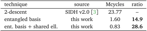
construc-tion during decompression, we introduce theshared El-ligatortechnique. This technique allows for a 1.5−2.8× faster ternary basis generation compared to the previous plain generation technique from[3]. When the new en-tangled basis generation is coupled with shared Elligator, the improvements are even more significant attaining a 29.9× speed up. For example, our implementation achieves 0.83M cycles for a 2m-torsion basis generation,
purpose. The previous 2-descent technique has a cost of 23.77M cycles according to our experiments.
• Computing discrete logarithms. Inspired by De Feo et
al.’s optimal strategy method to compute smooth-degree isogenies [6], we propose an algorithm to com-pute discrete logarithms in the group µ`n given an
efficient method to compute discrete logarithms in µ` where`is a small prime, or more generally, an algorithm to compute discrete logarithms in the group µ(`w)n/w
when w | n, given an efficient method to compute discrete logarithms in µ`w. For instance, forw=6 our
algorithm is 3.9× and 4.6× faster than the algorithm used by[3]for the groupsµ2372andµ3239 respectively. • We further describe how to compute Pohlig-Hellman in
the groupµ`nfrom an adaptation of the optimal strategy
traversal, given an efficient method to compute discrete logarithms in the groupµ`w whenw-n.
• Pairing computation. We exploit the special shapes of
pairs of points generated as entangled bases and the existence of a subfield dismissed by [3] to optimize the Tate pairing. We achieve a speedup of 1.4×for the pairing phase over the algorithms used by[3]for both binary and ternary pairings.
• We evaluate the impact of our improved key compres-sion on the Supersingular Isogeny Key Encapsulation (SIKE) scheme [7], a recently submitted candidate to NIST’s call for standardization of post-quantum cryptog-raphy.
• Other improvements. We introducereverse basis decom-position, which combined with the previous improve-ments, allows for further optimizations of compression and decompression. For example each party only needs to compute 4 pairings rather than 5. Also, two expensive cofactor multiplications by 3n are saved during Bob’s
compression, and one cofactor multiplication by 3n is
saved during Alice’s decompression.
We have implemented the above improvements on top of (the then-latest version of) the Microsoft SIDH library [8]. The library is designed for the specific prime p =23723239−1 of size logp=751 bits.
Our software can be found at https://github.com/ geovandro/PQCrypto-SIDH/releases/tag/1.1.0.
1.1 Notations and conventions
For simplicity, we assume that finite field arithmetic is carried out in a base fieldFpand its quadratic extensionFp2for a prime
pof form p:=2m·3n−1 for somem>2 andn>1, so that
p≡3(mod 4). The quadratic extensionFp2/Fp is represented
as Fp2 =Fp[i]/〈i2+1〉, and arithmetic closely mimics that of
the complex numbers.
All curves are represented using the Montgomery model unless otherwise specified. We follow the convention of using subscriptsAandBfor Alice and Bob, respectively. For example, the secret isogeny φA is computed by Alice and her public
parameters are denoted by the points PA,QA and the curve
EA. Similarly, Bob’s isogeny is denoted by φB, and his public
parameters arePB,QB,EB.
We denote byi,c,m,s, andathe costs of inverting, cubing, multiplying, squaring, and adding/subtracting/shifting inFp,
respectively, and by I, C, M, S, and A the costs of the corre-sponding operations inFp2. We disregard the cost of changing
a sign (for instance, when handling the conjugate of a field element). The costs of theFp2operations relative to the costs of
operations inFpcan be approximated by 1I=1i+2m+2s+1a,
1C=2m+1s+4a, 1M=3m+5a, 1S=2m+3a, and 1A=2a, by using the finite-field analogues to well-known Viète multiple-angle trigonometric identities[9, Formulas 5.68 and 5.69].
2 Reverse basis decomposition
In this section, we use reverse basis decomposition to speed up both Alice’s and Bob’s key compression by saving one pairing computation. Later in Section3.1we show that, when combined with an entangled basis generation, this technique will allow for avoiding two cofactor multiplications by 3n in
Bob’s key compression and one in Alice’s key decompression. We prove our results from Alice’s point of view. The proofs for Bob are similar.
The main previous idea to achieve key compression
[2], [3] is the following: instead of transmitting points
φA(PB),φA(QB)∈EA[3n], which are represented by two
abscis-sas inFp2and consume 4 logpbits, Alice computes a canonical
basisR1,R2∈EA[3n]and expresses the expanded public key in
that basis asφA(PB) =a0R1+b0R2andφA(QB) =a1R1+b1R2.
In matrix notation,
φ
A(PB)
φA(QB)
=a0 b0
a1 b1 R
1
R2
. (1)
This representation consists of four smaller integers (a0,b0,a1,b1)∈(Z/3nZ)4of total size 2 logpbits as suggested
in[2]. This was improved in[3]by transmitting only the triple (a−01b0,a−01a1,a−01b1) ∈ (Z/3nZ)3 or (b0−1a0,b0−1a1,b−01b1) ∈
(Z/3nZ)3 depending on whether a0 or b0 is invertible.
There-fore, only (3/2)logp, plus one bit indicating the invertibility of a0 or b0 modulo 3n, is needed. In the above mentioned
techniques, the coefficientsa0,b0,a1,b1can be computed using
five Tate pairings given by
g0=e3n(R1,R2)
g1=e3n(R1,φA(PB)) =e3n(R1,a0R1+b0R2) =g
b0 0
g2=e3n(R1,φA(QB)) =e3n(R1,a1R1+b1R2) =g
b1 0
g3=e3n(R2,φA(PB)) =e3n(R2,a0R1+b0R2) =g−
a0 0
g4=e3n(R2,φA(QB)) =e3n(R2,a1R1+b1R2) =g−
a1 0 .
(2)
From this, Alice can recovera0,b0,a1, andb1by solving discrete
logs in a multiplicative subgroup of smooth order 3nusing the
Pohlig-Hellman algorithm.
Now sinceφA(PB)andφA(QB)also form a basis forEA[3
n],
we see that the coefficient matrix in (1) is invertible modulo 3n.
So, we can write
R1
R2
=
c0 d0
c1 d1 φ
A(PB)
φA(QB)
3
by inverting the matrix in (1). Changing the roles of the bases {R1,R2}and{φA(PB),φA(QB)}in (2) we get
h0 =e3n(φA(PB),φA(QB))
h1 =e3n(φA(PB),R1)
=e3n(φA(PB),c0φA(PB) +d0φA(QB)) =h
d0 0
h2 =e3n(φA(PB),R2)
=e3n(φA(PB),c1φA(PB) +d1φA(QB)) =h
d1 0
h3 =e3n(φA(QB),R1)
=e3n(φA(QB),c0φA(PB) +d0φA(QB)) =h−
c0 0
h4 =e3n(φA(QB),R2)
=e3n(φA(QB),c1φA(PB) +d1φA(QB)) =h−
c1 0 .
(4)
The first pairing in (4) is computed as h0 = e3n(PB, ˆφA◦
φA(QB)) = e3n(PB,[degφA]QB) = e3n(PB,QB)2 m
, which only depends on the public parameters PB,QB and m. Therefore,
it can be computed once and for all and be included in the public parameters. In particular, only the pairings h1,h2,h3
and h4 need to be computed at runtime. The discrete logs
are computed as before using Pohlig-Hellman, yielding c0 =
−logh
0h3,d0=logh0h1,c1=−logh0h4 andd1=logh0h2. Next,
Alice inverts the computed coefficients matrix of (3) to obtain the coefficient matrix of (1). Explicitly,
a0 b0
a1 b1
= 1 D
d1 −d0
−c1 c0
where D=c0d1−c1d0. Notice that the extra inversion ofD−1
does not need to be carried out when using the technique in
[3]. More precisely, since at least one ofd0 and d1, sayd1, is
invertible modulo 3n, Alice transmits the tuple
(a−01b0,a0−1a1,a−01b1)
= (−d1−1DD−1d0,−d1−1DD− 1c
1,d1−1DD− 1c
0)
= (−d1−1d0,−d1−1c1,d1−1c0)
which is independent ofD.
3 Entangled basis generation
We now introduce a technique to create a complete basis of the 2m-torsion from a single (albeit specific) point of order
2m. In other words, the cost involved is essentially that of
creating a generator for a single subgroup of order 2minE[2m]:
a generator for the linearly independent subgroup becomes immediately available almost for free. Consequently, the linear independence test consisting of two scalar multiplications by 2m−1 can be avoided. This is akin to distortion maps even
though none is typically available for the curves involved in SIDH. We call the resulting bases “entangled” by analogy with the quantum phenomenon whereby the properties of one entity are entirely determined by the properties of another entity despite their separation1.
In order to build an entangled basis〈P,Q〉=E[2m]for E :
y2=x3+Ax2+x, we somewhat “subvert” the original Elligator 2 formulas [10] under a different motivation than encoding points to random strings: obtaining two linearly independent points onEat once. Herein the valuet:=u0r, foru0∈Fp2\Fp
andr∈F∗ps.t.u:=u 2
0∈Fp2\Fp, will be a square rather than a
non-square. The new construction is proved in Theorem1.
1. We stress, however, that here the naming is purely analogous: there is no quantum process involved in the construction.
Remark. As in[10]we assume thatA6=0 in the Montgomery model. The caseA=0 corresponds to the curveE:y2=x3+x which is used as the initial curve in most of the implemen-tations. This does not pose a problem in our setting. This is because first, runtime basis generation does not happen for the initial curveE, and second, the probability thatEis encountered in the middle of the key exchange is negligible. So the parties can avoid this issue by checking the j-invariant of their public keys.
Theorem 1. Given a Montgomery supersingular elliptic curve EA/Fp2: y2=x(x2+Ax+1)where p=2m·3n−1,#EA(Fp2) =
(p+1)2, and A6= 0, let t ∈ Fp2 be a field element such that
t2 ∈
Fp2\Fp, and let x1 := −A/(1+t2) be a quadratic
non-residue that defines the abscissa of a point P1 ∈ EA(Fp2). Then
x2:=−x1−A defines the abscissa of another point P2∈EA(Fp2)
such that〈[h]P1,[h]P2〉=EA[2m], where h:=3nis the cofactor
of the2m-torsion group.
Proof. Since x2 = t2x1, both abscissas are quadratic
non-residues and by [11, Chapter 1 (§4), Theorem 4.1] the two pointsP1= (x1,y1),P2= (t2x1,t y1), with x1+t2x1+A=0,
are not in [2]EA. So the points [h]P1 and [h]P2 are full 2m
-torsion points. To prove thath·P1,h·P2 generate EA[2m]we
have to prove that[h·2m−1](P
1−P2)6=0, or equivalently that
(u,v) =P1+ (−P2)6∈[2]EA.
By the addition law[12, Algorithm 2.3]onEAwe get
λ= y2−y1
x2−x1
=−t y1−y1
t2x 1−x1
=−(t+1)y1
(t2−1)x 1
= −y1
(t−1)x1
,
µ= y1x2−y2x1
x2−x1
= t(t+1)y1x1
(t+1)(t−1)x1
=−λt x1,
u=λ2−A−x1−x2=λ2,
v=−λu−µ=−λu−(−λt x1) =−λ(u−t x1).
From the above equalities we see that v2 = λ2(u−t x1)2 =
u(u2+Au+1) and henceu2+Au+1= (u−t x1)2. Let w:=
u−t x1 =
p
u2+Au+1. Then 1−(u−w)2 =1−t2x2 1 =x
2 1+
Ax1+1, which is a quadratic non-residue because x1is itself a
quadratic non-residue while their product is obviously a square, x1(x21+Ax1+1) =y12. A straightforward calculation shows that
(1−(u+w)2)(1−(u−w)2) =u2(A2−4). ButA2−4 is a quadratic residue sinceEAhas the full 2-torsion overFp2. Therefore, both
(u±w)2−1 have the same quadratic residuosity, that is, they are both quadratic non-residues by the above.
Now2assume by contradiction thatP
1−P2∈[2]EA, i.e. there
is a point(x,y)∈EA(Fp2)such that[2](x,y) = (u,v). From the
doubling formula onEAwe get
u= (x
2−1)2
4x(x2+Ax+1).
From this we get a quartic equation(x2−1)2−4ux(x2+Ax+1) =
0. Since x 6=0, we can divide both sides by x2 and rearrange some terms to get
x+1
x 2
−4u
x+1 x
−4(Au+1) =0.
From this we obtain
x+1 x=
4u±p
16(u2+Au+1)
2 =
4u±4w
2 =2(u±w).
In turn, from this we get x2−2(u±w)x+1=0. Again since x ∈ Fp2, the discriminant 4(u±w)2−4, and hence at least
one of the (u±w)2−1 must be a quadratic residue. But this
contradicts the earlier observation that (u±w)2−1 are both quadratic non-residues. Therefore P1−P2 6∈[2]E, yielding the
claim that〈[h]P1,[h]P2〉=EA[2m].
In practice, one can efficiently implement entangled basis generation as follows. Let u0 ∈ Fp2\Fp such that u := u20 ∈
Fp2\Fp, e.g.u0=1+iandu=2i. Define two separate tables of
pairs(r,v)withv:=1/(1+ur2):
• tableT1contains pairs(r,v)in whichvis quadratic
non-residue,
• table T2 contains pairs (r,v) in which v is quadratic
residue.
Performing one quadraticity test onA, only once per curve, and restricting table lookup to the table of opposite quadraticity ensures that x:=−Av is a non-square. Repeating quadraticity tests to ensure that a corresponding y exists, and completing one square root extraction inFp2to obtain y, one gets 2 points
whose orders are multiples of 2m at once. This is detailed in
Algorithm3.1.
Let us compare the number of operations required by the entangled basis algorithm with the plain basis generation algo-rithm used in Costelloet al.[3].
Entangled basis: testing the quadraticity ofAtakes(m+n+ 1)s+nm. The main loop runs twice on average at a cost 2(m+n+1)s+ (2n+22)m. The last stage is to complete a square root and costs(m+n−1)s+ (n+1)m+1i. The total cost of the algorithm is then
(4m+4n+2)s+ (4n+23)m+1i.
Plain basis: To get the abscissa of a point on the curve takes (2n+22)m+2(m+n+1)s. Clearing the cofactor 3nrequires
npoint triplings at a cost 32nm. We also need to compute m−1 point doublings for linear independence check that is required in the next steps. So obtaining the first basis point costs(34n+16m+6)m+2(m+n+1)s. The second basis point is obtained exactly the same way, except we also need a linear independence check. This is done in loop that runs twice on average. The expected cost of obtaining the second point is then twice the cost of obtaining the first point including the them−1 doublings step. The last stage of the algorithm is to recover theycoordinates of the points which costs(4m+4n)s+ (4n+36)m+2i. Adding all these, the total cost of the algorithm is
(10m+10n+6)s+ (48m+106n+54)m+2i.
For the valuesm=372 and n=239, and assumings=0.8m
andi=100m, we get the performance ratio of 15.92.
3.1 Avoiding cofactor multiplication
Combining reverse basis decomposition and entangled basis generation enables us to further avoid two scalar multiplica-tions by the large cofactor 3n during Bob’s public key
com-pression, and one during Alice’s decompression. First notice that Algorithm 3.1 already incorporates the mentioned opti-mization, i.e. the output points S1 and S2 satisfy (R1,R2) :=
([3n]S
1,[3n]S2)such that〈R1,R2〉=E[2m]. This is only
possi-ble because in reverse basis decomposition the Tate pairings
Algorithm 3.1 Entangled basis generation for E[2m](
Fp2) :
y2=x3+Ax2+x
INPUT: A=a+bi ∈Fp2; u0 ∈Fp2 : u=u20 ∈ Fp2\Fp; tables
T1,T2 of pairs(r ∈Fp,v=1/(1+ur2)∈Fp2)of QNR and
QR.
OUTPUT: {S1,S2}such that〈[3n]S1,[3n]S2〉=E[2m](Fp2).
1: z←a2+b2, s←z(p+1)/4
2: T ← (s2 =? z) T
1 : T2 // select proper table by testing
quadraticity ofA 3: repeat
4: lookup next entry(r,v)fromT 5: x← −A·v //NB:xnonsquare
6: t←x·(x2+A·x+1) //test quadraticity oft=c+d i 7: z←c2+d2, s←z(p+1)/4
8: untils2=z //computey←px3+A·x2+x
9: z←(c+s)/2, α←z(p+1)/4, β←d·(2α)−1
10: y←(α2 ?=z)α+βi:−β−αi //compute basis
11: returnS1←(x,y),S2←(ur2x,u0r y)
hi take the points Si in their second argument which does
not need to be necessarily cofactor-reduced. In this case, for R1=c0φB(PA) +d0φB(QA)andR2=c1φB(PA) +d1φB(QA), the
respective pairing computations are
k0 = e2m(φB(PA),φB(QA))
k1 = e2m(φB(PA),S1)
= e2m(φB(PA),[3−n]R1) =k
3−nd
0 0
k2 = e2m(φB(PA),S2)
= e2m(φB(PA),[3−n]R2) =k
3−nd
1 0
k3 = e2m(φB(QA),S1)
= e2m(φB(QA),[3−n]R1) =k−
3−nc
0 0
k4 = e2m(φB(QA),S2)
= e2m(φB(QA),[3−n]R2) =h−3
−nc
1 0 .
Thus, the discrete logarithms are the desired ones up to a factor 3−n, and given by ˆc0=−logk0k3=3
−nc
0, ˆd0=logk0k1=3 −nd
0,
ˆ
c1 = −logk0k4 = 3 −nc
1, and ˆd1 = logk0k2 = 3 −nd
1. Notice
that 3−nmod 2m must be odd which implies that ˆc 0 or ˆd0
is invertible if and only if c0 or d0 is invertible. Similar to
the situation in Section 2, when using the compression with only 3 coefficients as in[3]Bob transmits exactly the original coefficients: assuming ˆc0is invertible, then
(ˆc−10 dˆ0, ˆc0−1ˆc1, ˆc0−1dˆ1)
= (c−013n3−nd 0,c0−13
n3−nc 1,c0−13
n3−nd 1)
= (c−01d0,c0−1c1,c0−1d1)
The derivation whend0is invertible is analogous.
To decompress Bob’s public key, Alice needs to perform a single cofactor multiplication by 3n as follows. Assume
that a0 is invertible modulo 2m so that Alice receives the
triple(a0−1b0,a0−1a1,a0−1b1). She needs to compute the kernel
ker(φAB) = 〈φB(PA) +skA·φB(QA)〉 which can be written
as 〈a0R1+b0R2+skA·(a1R1 +b1R2)〉 = 〈(a0 +skAa1)R1+
(b0+skAb1)R2〉 As noted in [3], one computes ker(φAB) as
a−01ker(φAB) =〈(1+skAa−
1
0 a1)R1+(a0−1b0+skAa−
1
0 b1)R2〉, which
can be done with one scalar multiplication and one point addition by writing ker(φAB) =〈R1+ (1+skAa0−1a1)−1(a−01b0+
skAa−
1
0 b1)R2〉. Now if Alice uses Algorithm3.1, she obtains an
5
She can then compute T = 〈S1+ (1+skAa0−1a1)−1(a−01b0+
skAa−
1
0 b1)S2first and then recover the correct kernel ker(φAB) =
〈[3n]T〉by performing one cofactor scalar multiplication.
4 On basis generation for
E
[
3
n]
The entangled basis approach introduced in Section3does not immediately generalize to the ternary case. There is no clear way to simultaneously choose two linearly independent points. As a consequence, to generate bases for E[3n] we adopted
the naïve approach of randomly picking candidate points and testing them for the correct order and linear independence.
Costelloet al.suggest the use of a 3-descent approach based on a result by Schaefer and Stoll [5], and claim significant performance gains. However, we were unable to reproduce and thus verify their claims. On the contrary, the naïve method is observed to be always faster than 3-descent, with a cost ratioCnaïve/C3-descent≈0.89 that runs against their claim. The
following detailed analysis appears to corroborate this observed cost ratio.
In Costello et al.’s 3-descent approach, the claimed gains only apply totestingwhether a point is inE\[3]E. We note that the cost of generating candidates for testing has to be taken into account as well.
Thus, on the one hand, naïve testing involves:
• one Elligator construction at a costLper attempt, • mdoublings at a costDeach per attempt, • n−1 triplings at a costTeach per attempt,
• 9/8 attempts on average at a costPeach to get a point
of right order,
• 4/3 point constructions and checks at a costCeach on
average to get a second, linearly independent point.
Hence the naïve cost to get (the x-coordinates of) the base points is(1+4/3)(9/8)P+ (4/3)C, complemented by two curve equation solvings at a costEeach to complete the point coordinates, or(1+4/3)(9/8)P+ (4/3)C+2Eoverall.
EstimatingL= (0.8m+1.8n+9.8)m+20a,D=13m+29a,
T=27m+61a,C=2(3m+5a),E=1i+(1.6m+3.6n+27.6)m+
46a, and noticing thatP=L+mD+ (n−1)T, we conclude that the naïve cost isCnaïve ≈2i+ (39.425m+82.8n+18.05)m+
(76.125m+160.125n−3.708)a.
On the other hand, the 3-descent method initially involves:
• one Elligator construction at a costL, • mdoublings at a costD,
• n−1 triplings at a costT,
• one curve equation solving at a costE,
• one filter function construction at a costFto get a point
P3of order 3 and possibly the first base point.
Note that a more expensive doubling formula at a cost D0 =
16m+34a(instead ofD=13m+29a) was employed by[3]
which takes the curve coeficients in projective form. This pro-jective formula is useful for computing propro-jective 2m-isogenies
but we note that it is not necessary in the context of basis generation and one can simply stick to the usual more efficient Montgomery doubling[13]. We consider the faster version in our estimates.
The 3-descent method will require (with probability 1/9) an extra, filtered point construction at a costZto get the first base point, plus 4/3 filtered point constructions and checks on
average (since the probability of check success is 3/4) to get the second base point, and finally two curve equation solvings. Estimating F = 1i+12.6m+29a, Z = 3i+ (17.8m+ 37.8n+39.3)m+ (29m+61n+57.5)a, and keeping the same remaining estimates as before, we conclude that the 3-descent cost isC3-descent:= (3(4/3) +3(1/9) +4)i+ ((17.8m+37.8n+
45.3)(4/3) + (17.8m+37.8n+39.3)(1/9) +31.2m+39.6n+ 78.2)m+((29m+61n+67.5)(4/3)+(29m+61n+57.5)(1/9)+ 29m+61n+126)a.
This yields a cost ratioCnaïve/C3-descent≈0.89, which is what
we observe experimentally. This runs against the claim in[3]on “the significant speed advantage that is obtained by the use of the result of Schaefer and Stoll[i.e. the 3-descent method]:” the naïve method is observed to be always faster than 3-descent.
4.1 Shared Elligator and faster decompression
Although shown to be faster than 3-descent in the previous section, the naïve approach for basis generation ofE[3n]incurs a substantial cost that seems unavoidable at key compression. Interestingly, the knowledge gained in the process (in the form of the actual countersr that specify the points in the Elligator 2 construction) could be then shared between Alice and Bob, speeding up the latter’s work at key decompression. For a very modest increase in Alice’s public key size (for instance, a single extra byte for each of the two basis points would provide space that is only exceeded with probability well below 2−400), Bob’s E[3n]basis generation would get about 32% faster, and his full
decompression of Alice’s key would become about 24% faster. As discussed in Section 4, naïve E[3n] basis generation
requires 9/8 construction attempts on average to get each point of right order individually, and the second point construction and testing has to be repeated 4/3 times on average to ensure the pair constitutes a basis. This means that, if the cost of generating each point candidate isP, the actual expected cost to obtain a basis is roughly(21/8)P+(4/3)C+2E. In case Alice shares the actual Elligator 2 counters that lead to a basis, the cost for Bob would become 2P+C+2Esince both the Elligator computation and the linear independence test would become deterministic. This represents a speed up of about 1.47× (or 32% faster) on basis generation alone and 1.4×for the overall decompression compared to the 3-descent method suggested in
[3].
Remark. Notice that if Bob trusts Alice, i.e., the Alice’s pub-lic key is authenticated, then n−1 triplings can be avoided since linear independence test is not necessary (the Elligator counters are supposed to give a genuine basis). In this case the improvement is more drastic, the cost to generate a basis for E[3n]becomes 2P0+2EwhereP0=L+mDwhich represents a
speedup of 2.86×over the previous 3-descent approach. In this case, the task of decompression would get about 2×faster.
Moreover, the Elligator 2 counters tend to be very small. Specifically, if the probability that a point candidate is rejected at a certain attempt is 1/t, then the expected number of attempts is t/(t−1) and the probability that the number of attempts exceeds N is the probability of failing N times, i.e., t−N. For the first point, t=9 (only one of the 9 points of
3-torsion causes rejection when computing[3n−1]R), while for the
second pointt=3 (because the probability of a candidate being accepted at a certain attempt is(8/9)(3/4) =2/3, and hence the probability of rejection is 1/3). Therefore, for the first point the expected number of attempts is 9/8 and the probability that the number of attempts exceeds N is 9−N, while for the
second point the expected number of attempts is 3/2 and the probability that the number of attempts exceedsN is 3−N. If we
use one byte for each counter (interpreted as an index to a table of squares or a table of non-squares), the probabilities that the available counter space (N=255) is exceeded are a whooping 2−811.5and 2−404.2respectively. This means that Alice needs to transmit just two more bytes with her key.
This modest increase in Alice’s key size is compensated by worthwhile speed-ups for Bob. Form=372 andn=239, Alice’s extended key size becomes 330 bytes rather than 328 (see Table 3 in[3]), matching Bob’s plain key size. While the 3n-torsion generation time for Alice is that indicated on Table 5, Bob’s time decreases to about 13.63 Mcycles yielding a ratio 1.47 rather than 1.15. Furthermore, Alice’s compression ratio to the previous state of the art stays the same as well, but Bob’s ratio improves from 1.09 to 1.30.
4.2 The Shared Elligator on Entangled Bases
Interestingly, the binary entangled basis generation technique not only allows for a shared Elligator decompression but in addition requires less extra bandwidth compared to the ternary case, i.e., 1 instead of 2 extra bytes. In addition, the result-ing 50% faster decompression is considerably more noticeable compared to the ternary counterpart. The reason for this bigger improvement is that the Step 1 of the entangled basis Algorithm
3.1consisting of a relatively expensive quadraticity test can be avoided. In this case, Bob who is responsible for compressing his key in the 2m-torsion can transmit the quadraticity of A
through a single bit b. Since Bob’s public key size is not an exact multiple of 32 bytes for a 751-bit prime, a few unused bits in the byte-oriented representation of the key are available and one of those can be used for transmitting this information aboutA.
The other information Bob can share with Alice is the counterrcomputed in Step 4 that leads to a point on the curve for the first candidate. This can be done with one single extra byte. The probability of exceeding one byte is the probability of the first abscissa failing to be on the curveN=255 times, i.e., 2−N=2−255. Moreover, because the second point on an
entan-gled basis is determined by the first point, no second extra byte is necessary in this case. Algorithm4.1describes the entangled basis generation with shared Elligator for decompression.
Entangled basis+shared Elligator: The resulting operation count for the entangled basis generation coupled with shared Elligator involves only one single iteration of the loop in Step 3 of Algorithm 3.1 amounting to (m+n+ 1)s+(n+9)mand the final part (Steps 8 to 10) amounting
Algorithm 4.1Entangled basis generation coupled with shared Elligator forE[2m](
Fp2): y2=x3+Ax2+x
INPUT: A=a+bi ∈Fp2; u0 ∈Fp2 : u=u20 ∈ Fp2\Fp; tables
T1,T2 of pairs(r ∈Fp,v=1/(1+ur2)∈Fp2)of QNR and
QR. A bitbi tforA’s quadraticity andr∈Fp.
OUTPUT: {S1,S2}such that〈[3n]S1,[3n]S2〉=E[2m](Fp2).
1: T←(bi t=? 1)T1:T2 //select proper table according to
A’s quadraticity
2: x← −A·T[r] //NB:xnonsquare
3: t←x·(x2+A·x+1) //test quadraticity oft=c+d i 4: z←c2+d2, s←z(p+1)/4
5: ifs26=zthen
6: Abort //incorrect parameters(b,r)received 7: end if //compute y←px3+A·x2+x
8: z←(c+s)/2, α←z(p+1)/4, β←d·(2α)−1
9: y←(α2 ?=z)α+βi:−β−αi //compute basis
10: returnS1←(x,y),S2←(ur2x,u0r y)
to(m+n−1)s+ (n+6)m+i. Adding up the above costs, the new basis generation will cost
2(m+n)s+ (2n+15)m+i.
Assumingi=100mands=0.8m, this represents a speed up of 29.9×faster basis generation compared to the plain basis generation described in Section3.1.
5 Pairing computation
The pairing computation techniques by Costello et al.[3]are based on curves in a variant of the Montgomery model, with projective coordinates(X2,X Z,Z2,Y Z), which turned out to be the best setting among several models they assessed. We will argue that the older and today less favoured short Weierstraß model leads to more efficient pairing algorithms.
Interestingly, Costelloet al.dismiss the technique of denom-inator elimination[14]and keep numerators and denominators separate during pairing evaluation. We point out, however, that pairing values are defined over Fp2 and the inverse of
a field element a+ bi is (a−bi)/(a2 +b2). Hence, rather than keeping a separate denominator a+bi one can simply and immediately multiply the pairing value by the conjugate a−biinstead; the result only differs from the original one by a denominator consisting of the norm a2+b2 ∈
Fp, and this
denominator does get eliminated by the final exponentiation in the reduced Tate pairing computation. This leaves the cost of pairing computation unchanged, but it simplifies the imple-mentation as it entirely does away with separate numerators and denominators.
Letr≥0 be the pairing order. For embedding degreek=1, r |Φ1(p2) =p2−1=2m·3n·(p−1), and by construction r
is always either 2m or 3n. We will be interested in computing
reduced Tate pairings of order r, whose first argument must have that order as well. In the case of compressed SIDH keys, pairings of the following forms are computed together (recall that a fifth pairing e0 := er(P,Q) = er(P0,Q0)degφ is readily
available through precomputation):
e1:=er(P,R1),e2:=er(P,R2),
7
where the first two pairings share the same first argument P, and next two pairings share the same first argumentQ.
From now on, we will split the discussion into two cases: binary-order pairings, r=2m, and ternary-order pairings, r=
3n. The curve equation in the short Weierstraß model is E W :
v2=u3+au+b. Given a Montgomery curve EM : y2 =x3+
Ax2+x, the corresponding short Weierstraß model is obtained viaa=1−A2/3, b= (2A3−9A)/27, and a point(x,y)∈E
M
maps to a point(u,v)∈EW by settingu=x+A/3, v=y. For
convenience, we extend Jacobian coordinates[X :Y :Z]with a fourth component,[X:Y:Z:T]withT=Z2.
5.1 Binary-order pairings
The computation of the reduced Tate pairinger(P,Q)of order
r=2mproceeds as described in Algorithm5.1, which requires
doubling a pointV∈E(Fp2). The doubling formulas in Jacobian
coordinates have a single exception, that occurs when the point being doubled has order 2. That is, when y = 0, since the angular coefficient of the tangent to the curve at that point becomes undefined. That exception, however, can only occur deterministically in the scenario contemplated here, namely at the last step of the Miller loop; since by definition the first pairing argument is always a point of order 2m, chosen by the
very entity that is computing the pairing.
Besides, the difference in runtime reveals no private infor-mation, since the pairing arguments are either already public for being part of a conventional torsion basis, or else are about to be made public for being part of a public key.
Algorithm 5.1Tate2(P,Q): basic reduced Tate pairing of order r=2m:
INPUT: pointsP,Q. OUTPUT: er(P,Q).
1: f ←1, V←P 2: fori←0tom−1do
3: f ←f2·g
V,V(Q)/g[2]V(Q), V ←[2]V
4: end for
5: returner(P,Q)←f(p 2−1)/r
In Algorithm5.1, the functiongU,Vis defined to be the lines
throughU and V. IfU=V thengU,V is the tangent atU, and
if either U =∞ orV = ∞then gU,V is the vertical line at
the other point. Also we denote by gU the value gU,−U. The
most efficient doubling algorithm for (either plain or modified) Jacobian coordinates appears to be one devised by Bernstein and Lange[15], which maintains an additional coordinateU:= aZ4. However, that algorithm does not directly compute the value ofT=Z2that will be needed for pairing calculation. We will thus modify the Bernstein-Lange formulas so that the cost of recoveringT is less than that of squaringZ.
Let V = [X :Y : Z:U :T]and[2]V = [X0 :Y0 :Z0:U0 : T0] in the extended coordinate system defined above. Then, initializingT←Z2andU←aT2:
X2←X2; Y2←Y2; W ←2Y2; W2←W2;
M←3X2+U; S←(X+W)2−X2−W2;
X0←M2−2S; Y0←M·(S−X0)−2W2;
Z0←(Y+Z)2−Y2−T; T0←(Z0)2; U0←4W2·U;
The cost is 2M+7S+16A=20m+63a. This is only 1m+5a
more than the cost 3M+5S+14A=19m+58a of doubling without yieldingZ2as a by-product.
This algorithm yields the intermediate values λN := M, λD := Z0 =2Y Z, W, and Y2, besides the point coordinates.
These values, together with L←Z0·T,R←Z0·T, are useful¯ in the calculation of a function equivalent to gV,V(Q)/g[2]V(Q),
namely ˜g2(V,Q):= (M·(T·x−X) +W−L·y)·R·(T0·x−X0)−
when V 6= O and [2]V =6 O (i.e. Z 6= 0 and Z0 6= 0), ˜
g2(V,Q):= (T·x−X)·T¯ when V =−V 6=O(i.e.Z 6=0 and
Z0=0), or simply ˜g2(V,Q):=1 whenZ=O. Denominators in
the base field, namely|Z2·(T0·x−X0)|2∈
Fpin the first case
and|Z2|2∈
Fpin the second case, are eliminated.
Since the scenario where the pairing computations take place only involve bases of the 2m-torsion group, and hence
points of full order 2m, the exceptional formula is indeed never
invoked until the end of Miller’s loop. The difference in process-ing time is irrelevant for security here, since the computations only involve information that is meant to be public.
However, one can further optimize the computation of (a function equivalent to) ˜g2(V,Q). First, the expression(T0·x−X0)
that occurs at a certain step will play the role of(T·x−X)at the next step, so one can simply store it from one step to the next and thus save 1M. Second, one can show that allRand ¯T factors that appear in the definition of ˜g2(V,Q)are irrelevant to
the pairing value, and can be omitted. We provide the details in the Appendix B.
Consequently, initializingh←T·x−X before Miller’s loop at a cost of 1Mper pairing, the line function value g can be evaluated as
g←M·h+W−L·y; h←T0·x−X0; g←g·¯h
at a cost of 4M+3A=12m+26a per step of Miller’s loop. The cost of computingL←Z0·T alone is 1M=3m+5a. This completes the construction of a line function ˆg2(V,Q)equivalent
to ˜g2(V,Q).
The updating of f at each step as f ← f2·ˆg2(V,Q)incurs
2m+3a to compute the complex square f2 plus 3m+5a to
compute f2·ˆg2(V,Q)from f2 and ˆg2(V,Q), totaling 5m+8a.
Therefore, the proposed variant has the following overall cost per step:
• (shared) cost of point doubling and line function
con-struction: 20m+63a+3m+5a=23m+68a;
• (individual) cost of line function evaluation and
accu-mulation: 12m+26a+5m+8a=17m+34a.
By comparison, the Costelloet al.[3]technique has the follow-ing costs:
• (shared) cost of point doubling and line function
con-struction: 9M+5S+1s+7a=37m+1s+67a;
• (individual) cost of line function evaluation and accu-mulation: 5M+2S+2s+1a=19m+2s+32a;
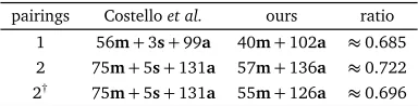
TABLE 1: Cost of the binary Miller loop (ratio assumess≈0.8m
and ignoresa).
pairings Costelloet al. ours ratio 1 56m+3s+99a 40m+102a ≈0.685 2 75m+5s+131a 57m+136a ≈0.722 2† 75m+5s+131a 55m+126a ≈0.696 †Simultaneous pairings on entangled bases
5.1.1 Pairings on an entangled basis
If two pairings e(P,R1), e(P,R2) sharing the same first
argu-ment P are computed on an entangled basis R1 = (x1,y1),
R2= (x2,y2)withx2=t2·x1, y2=t·y1, one can slightly
im-prove the line function evaluation and accumulation, exploiting the fact that multiplication by carefully chosen t or t2 given the values of T0·x1 or L·y1 is less expensive than the full
multiplicationsT0·x2orL·y2for generic(x2,y2).
Specifically, fort= (1+i)r andt2=2i r2 with some small r∈Fp, the cost of a dedicated implementation of simultaneous
pairings on entangled bases drops by 2m+10a, thus becoming only 55m+126a, or less than 70% the cost of the Costelloet al.method. The performance improvements brought about by the techniques we proposed are summarized on Table1. Our proposed variant of the simultaneous reduced Tate pairing is shown in full detail as Algorithm A.1 in the Appendix A.
5.2 Ternary-order pairings
The computation of the reduced Tate pairinger(P,Q)of order
r = 3n proceeds as described in Algorithm 5.2. Again, the
tripling formulas in Jacobian coordinates have an exception when y =0, but this can be handled in a similar fashion to the binary case. The difference in runtime reveals no private information for the same reason, namely only public data is involved in the pairing computations.
Algorithm 5.2Tate3(P,Q): basic reduced Tate pairing of order r=3n:
INPUT: pointsP,Q. OUTPUT: er(P,Q).
1: f ←1, V←P 2: fori←0ton−1do
3: f ←f3·g
V,V(Q)·gV,[2]V(Q)/(g[2]V(Q)·g[3]V(Q)),
4: V←[3]V 5: end for
6: returner(P,Q)←f(p 2−1)/r
The most efficient tripling algorithm known for Jacobian coordinates appears to be one devised by Bernstein and Lange [15]. Its cost is 6M+10S+25A =38m+110a for a curve with generic equation coefficients. We present a variant for the same modified Jacobian coordinates used in the binary case, with cost 5M+11S+31A=37m+120a.
LetV= [X:Y:Z:T:U]and[3]V= [X0:Y0:Z0:T0:U0] in the extended coordinate system as before. Then, initializing
T←Z2andU←aT2:
X2←X2; Y2←Y2; Y4←Y22;
M←3X2+U; M2←M2;
D←(X+Y2)2−X2−Y4; F←6D−M2;
F2←F2; W←2Y2; W0←2W; S←16Y4;
G←(M+F)2−M2−F2−S; G0←S−G;
H←2F2; H2←H2; H0←4G; F0←2F;
X0←(X+H)2−X2−H2−W0·H0;
Y0←2Y·(H0·G0−F0·H); Z0←(Z+F)2−T−F2;
T0←(Z0)2; U0←4H2·U
This algorithm yields intermediate values F, F0, G0, W, W0, and M, besides the point coordinates. These values, to-gether with L ← ((Y +Z)2 −Y2 −T)·T and R ← F ·T,¯
are useful in the calculation of a function equivalent to gV,V(Q)·gV,[2]V(Q)/(g[2]V(Q)·g[3]V(Q)), namely ˜g3(V,Q) :=
(M·h+d)·(G0·h+F0·d)·(W0·h+F)−·R·h¯3when[3]V6=O;
˜
g3(V,Q):= (M·h+d)·¯Lwhen[3]V =ObutV6=O; or simply
˜
g3(V,Q):=1 whenV=O, whereh:=T·x−X,d:=W−L·y,
h3:=T0·x−X0.
One can further optimize the computation of a function ˆ
g3(V,Q)equivalent to ˜g3(V,Q)in a similar fashion to what was
done for the binary case. First, the expression T0·x−X0 that occurs at a certain step will play the role ofT·x−Xat the next step, so one can simply store it from one step to the next and thus save 1M. Second, one can show that all Rand ¯L factors that appear in the definition of ˜g3(V,Q) are irrelevant to the
pairing value, and can be omitted. We give more details in the Appendix B.
Consequently, the parabola function construction can be completed by computing onlyLas above at a cost 1M+1S+3A. After initializingh←T·x−X before Miller’s loop at a cost of 1M per pairing, the value g of the parabola function can be evaluated as
d ← W−L·y;
g ← (M·h+d)·(G0·h+F0·d)·(W0·h+F); h ← T0·x−X0;
g ← g·¯h;
at a cost 9M+5A per step of Miller’s loop, except at the final step, when it is simply g ← M ·h+d. This completes the construction of a parabola function ˆg3(V,Q) equivalent to
˜ g3(V,Q).
The updating of f at each step as f ←f3·ˆg3(V,Q)incurs a
cost 1Cto compute the complex cube f3, plus 1Mto compute f3·ˆg3(V,Q) from f3 and ˆg3(V,Q). Therefore, the proposed
variant has the following overall cost per step, where again the shared part is amortized among simultaneous pairings that share the same first argument:
• (shared) cost of point tripling and parabola function construction: 5M+11S+31A+1M+1S+3A=40m+
134a;
• (individual) cost of parabola function evaluation and accumulation: 9M+5A+1C=32m+2s+66a.
9
TABLE 2: Cost of the ternary Miller loop (ratio assumes s≈ 0.8mand ignoresa).
pairings Costelloet al. ours ratio
1 103m+6s+188a 72m+2s+200a ≈0.683 2 137m+6s+248a 104m+2s+266a ≈0.756
• (shared) cost of point tripling and construction of the
parabola functions: 19M+6S+6s+15a=69m+6s+
128a;
• (individual) cost of evaluating the parabola functions
and accumulating the results: 10M+2S+4a=34m+
60a.
Therefore in the present case, where one has to compute pairs of pairings that share the same first argument, our technique costs a fraction ≈(40+2·33.6)/(73.8+2·34) = 107.2/141.8 ≈ 76% of the Costello et al. method, assuming 1s≈0.8mand essentially ignoringa.
The performance improvements brought about by the tech-niques we propose are summarized on Table2. Our proposed variant of the simultaneous reduced Tate pairing is shown in full detail in the Appendix as Algorithm A.2.
6 Discrete logarithm computation
Let L:=`w for some integer w>0, and letµLe ⊂Fp2 be the
set of Le-th roots of unity inFp2, i.e. µLe :={v ∈Fp2 | vL
e = 1}. Inverting inµLe is a mere conjugation,(a+bi)−1=a−bi
since the norm is 1. The Pohlig-Hellman method (Algorithm
6.1)[16], which computes the discrete logarithm of c ∈ µLe,
requires solving an equation of the form
rkLe−1−k=sdk
where s = gLe−1
has order L and, for k = 0, . . . ,e−1, dk ∈ {0, . . . ,L−1}is anL-ary digit,r0=c, andrk+1 depends onrk
anddk.
Algorithm 6.1 Basic Pohlig-Hellman discrete logarithm algo-rithm
INPUT: generatorg∈µLe, challengec∈µLe.
OUTPUT: d:=loggc, i.e.gd=c.
1: s←gLe−1
//NB:sL=1
2: d←0,r0←c
3: fork←0toe−1do
4: vk←rL
e−1−k
k
5: finddk∈ {0, . . . ,L−1}such thatvk=sdk
6: d←d+dkLk,rk+1←rk·g−L
kd k
7: end for //NB:gd=c
8: returnd
Assuming that g−Lk
is precomputed and stored for all k as a by-product of the computation of s, the naive strategy to obtain the discrete logarithm requires repeatedly computing the exponentialrLe−1−k
k at the cost ofe−1−kraisings to the L,
then solving a small discrete logarithm instance in a subgroup of order L to get one L-ary digit, then clearing that digit in the exponent ofrkat a cost not exceeding Lmultiplications to
obtainrk+1. The overall cost is thusO(e2).
It turns out that this strategy is far from optimal, as pointed out by Shoup[17, Chapter 11]. The crucial task is to obtain
the sequencer0Le−1,r1Le−2,r2Le−3, . . . ,reL−01in this order, since each rk depends on the previous one. We can visualize this task
using a directed acyclic graph∆strikingly similar to De Feoet al.’sTn graph, which they call a “discrete equilateral triangle”,
that models the construction of smooth-degree isogenies [6, Section 4.2.2].
In our case, the set of vertices is{∆j,k|j+k≤e−1}where ∆j,k := rL
j
k . Each vertex has either two downward outgoing
edges, or no edges at all. Vertices∆j,kwith j+k>e−1 have
two edges: a left edge ∆j,k →∆j+1,k that models raising the
source vertex to theL-th power to yield the destination vertex, rLj+1
k ← (r Lj
k )
L, and a right edge ∆j
,k → ∆j,k+1 that models
clearing the(j+k)-th digit in the exponent of the source vertex, rLj
k+1←rL
j
k ·g− L(j+k)d
k. Vertices∆j
,kwith j+k=e−1 are leaves
since they have no outgoing edges.
De Feo et al. [6, Equation 5] describe an O(e2) dynamic programming algorithm that computes the cost of an optimal subtree of ∆with root at ∆00 and covering all leaves. If the
cost of traversing a left or right edge is p or q respectively, and the cost of an optimal subtree of kedges is Cp,q(k), their
algorithm is based on the relations Cp,q(1) =0 and Cp,q(k) =
min1≤j<k Cp,q(j) +Cp,q(k−j) + (k−j)p+jq
fork>1.
The naive dynamic programming approach is to store the values of Cp,q(k) for k = 1 . . .e, invoking the above relation
k−1 times at each step to find the corresponding minimum, for a total e(e−1)/2 invocations, hence the O(e2)cost. However, because Cp,q(k) has no local minimum other than the single
global minimum (or two adjacent, equivalent copies of the global minimum at worst), one can find that minimum with a variant of binary search that compares two consecutive values near the middle of the search interval[1 . . .k−1]and then halves that interval. This yields theO(eloge) Algorithm
6.2, which computes Cp,q(k) and the structure of the optimal
traversal strategy by storing the values of j above that attain the minimum at each step.
Algorithm 6.2OptPath(p,q,e): optimal subtree traversal path
INPUT: p,q: left and right edge traversal cost; e: number of leaves of∆.
OUTPUT: P: optimal traversal path
1: Define C[1 . . .e] as an array of costs and P[1 . . .e] as an array of indices.
2: C[1]←0, P[1]←0 3: fork←2toedo
4: j←1, z←k−1 5: whilej<zdo
6: m←j+b(z−j)/2c, m ←m+1
7: t1←C[m] +C[k−m] + (k−m)·p+m·q
8: t2←C[ m ] +C[k− m ] + (k− m )·p+ m ·q
9: ift1≤t2 then
10: z←m
11: else
12: j← m
13: end if
14: end while
15: C[k]←C[j] +C[k−j] + (k−j)·p+j·q, P[k]←j 16: end for