Journal of Hydrology, Vol. 397 (1-2), 2011, pp. 1 – 9.
Published version can be downloaded from: http://dx.doi. o rg/10.1016/ j .jhydrol.2010.11.00 9 .
Testing the Structure of Hydrological Models using
Genetic Programming
Benny Selle
1and Nitin Muttil
2 1 Department of Primary Industries,Ferguson Rd, Tatura, Victoria 3616, Australia
2 School of Engineering and Science and Institute for Sustainability and Innovation Victoria University,
PO Box 14428, Melbourne, Victoria 8001, Australia
Abstract
Genetic Programming is able to systematically explore many alternative model structures of different complexity from available input and response data. We hypothesised that Genetic Programming can be used to test the structure of hydrological models and to identify dominant processes in hydrological systems. To test this, Genetic Programming was used to analyse a data set from a lysimeter experiment in southeastern Australia. The lysimeter experiment was conducted to quantify the deep percolation response under surface irrigated pasture to different soil types, water table depths and water ponding times during surface irrigation. Using Genetic Programming, a simple model of deep percolation was recurrently evolved in multiple Genetic Programming runs. This simple and interpretable model supported the dominant process contributing to deep percolation represented in a conceptual model that was published earlier. Thus, this study shows that Genetic Programming can be used to evaluate the structure of hydrological models and to gain insight about the dominant processes in hydrological systems.
1. Introduction
Typically, a hydrological model can be formulated as:
(
t)
tt
f
x
q
=
,
β +
ε
t=1, 2, …, n, (1)where t is a time interval, qt is the measured response of a hydrological system (such as
streamflow or deep percolation below the plant rootzone) predicted by function f ( ), xt is a
vector of inputs such as rainfall and potential evapotranspiration, β is a vector of model parameters and εtis an error. In this paper, f (xt, β) is referred to as model structure representing
hydrological processes contributing to response qt. The model structure is an important source
of uncertainty in hydrological predictions and should therefore be as rigorously tested as possible (Beven, 2001). The problem of identifying a model structure from an observed set of system inputs and responses has received considerable attention in control theory (see for e.g.
Ljung, 1999 and references therein) and statistics (see e.g. Breiman, 2001 and Chatfield, 1995, and the discussions therein). Particularly in statistics, it is often argued that there maybe multiple model structures that explain the observed data equally well and, at the same time, are physically plausible. While this is not necessarily a problem if the modelling purpose is prediction (as model predictions can be aggregated over a large set of competing models), it will represent an issue if the purpose of the modelling is system understanding. For most applications of hydrological models, a limited number of model structures are considered to be plausible. Consequently, only a few alternative model formulations are tested using some statistics of the model residuals ε such as the root mean square error. In addition to these statistics, model residuals should be checked for unexplained structure such as correlations with model inputs and variables that were not included in the model or trends to ensure that all information has been extracted from the available data (Kirchner et al., 1996). While few alternatives seem to be available for these tests based on model residuals, there is often limited rigor in unsystematically testing the structure of hydrological models. In particular, as complexity of models increases the problem of non-uniqueness of model structures increases, i.e. many different model structures having similar error statistics and characteristics (Beven and Freer, 2001). Conversely, for simpler models representing only a limited number of dominant processes, non-uniqueness is typically less problematic. However, as usually only a limited number of model structures are tested, it is difficult to know whether a robust, sufficiently simple model has been found and the dominant processes have been identified.
2. Material and Methods
Genetic programming
Genetic Programming (GP) is a relatively new automatic programming technique for evolving computer programs to solve, or approximately solve, problems (Koza, 1992). In engineering applications, GP is frequently applied to model structure identification problems. In such applications, GP is used to infer the underlying structure of either a natural or experimental process in order to model the process numerically. A number of applications of GP have been reported in water resources, which include rainfall-runoff modelling (Whigham and Crapper, 2001; Khu et al., 2001); effect of flexible vegetation on flow in wetlands (Babovic and Keijzer, 2000); analysis and prediction of algal blooms (Muttil and Chau, 2006; Muttil and Lee, 2005); flood routing in natural channels (Sivapragasam et al., 2008), real-time wave forecasting (Gaur and Deo, 2008), pedotransfer functions to estimate the saturated hydraulic conductivity (Parasuraman et al., 2007) and quantification of model structure uncertainty (Parasuraman and Elshorbagy,2008).
GP is a member of the Evolutionary Algorithm family, which are based upon concepts of natural selection and genetics. The basic search strategy behind GP is a genetic algorithm
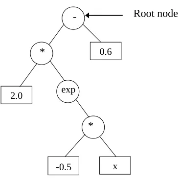
(Holland, 1975), although GP was developed much later (Koza, 1992). Like genetic algorithms, GP works with a number of solution sets, known collectively as a “population”, rather than a single solution at any one time; thus the possibility of getting trapped in a “local optimum” is avoided. GP differs from the traditional genetic algorithms in that it typically operates on “parse trees” instead of bit strings. A parse tree is built up from a “terminal set” (the input variables in the problem and randomly generated constants) and a “function set” (the basic operators used to form the GP model). The function set is user defined and can not only include algebraic operators, such as {+, -, *, /, exp, sin} but can also take the form of logical rules, making use of operators such as {IF, OR AND}. An example of a parse tree can be found in Figure 1, which is a parse tree representing the GP model f(x) = 2 * exp(-0.5 * x) - 0.6. The function set nodes are represented by circles and the terminal set nodes by rectangles. The “tree size” of this expression is 5, where “tree size” is the maximum “node depth” of a tree and “node depth” is the minimum number of nodes that must be traversed to get from the “root node” of the tree (see Figure 1) to the selected node.
INSERT FIGURE 1 NEAR HERE
population. This process of selection, reproduction and variation iterates until a user-defined “stopping criterion” is satisfied. The solutions in each iteration are collectively known as a “generation”. As the population evolves from one generation to another, new solutions replace the older ones and are supposed to perform better. The solutions in a population associated with the best fit individuals will, on average, be reproduced more often than the less fit solutions. This is known as the Darwinian principle of the “survival of the fittest”.
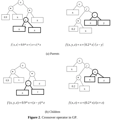
During each successive generation a proportion of the existing population is “selected” to breed a new generation. Individual solutions are selected through a fitness-based process, where fitter solutions are typically more likely to be selected. The next step is to generate a second generation population of solutions from those selected, through the two variation operators - crossover and mutation. Crossover is the random swapping of sub-trees between the selected “parent” parse trees to generate the new “children”. The crossover operator is demonstrated in Figure 2. It should be noted that bold parts of the two parent trees in Figure 2
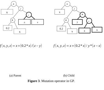
exchange each other to create the two children. The expressions for the 2 parents and the 2 children are also presented in this figure. The crossover tends to enable the evolutionary process to move toward promising regions of the solution space. In contrast to crossover, in mutation, a single parent parse tree is selected and random changes are made to it. Figure 3 illustrates one of the many possible mutation operators in GP, where an entire sub-tree in the parent is replaced by a randomly generated sub-tree to create the child. The mutation operator is introduced to prevent premature convergence to local optima. A high crossover rate is usually used so that the good characteristics (i.e., useful sub-trees) from the previous generations are transmitted to the new generation. On the other hand, the mutation rate is usually kept low since a high mutation rate can cause a big loss of useful sub-trees evolved in previous generations. This process of selection, reproduction and variation continues until a new population of solutions of appropriate size (which is the user defined “population size”) is generated. From generation to generation, the best solution evolved in previous generations is usually preserved, which is called “elitism”. For a detailed description of genetic programming from a water resources perspective, the interested reader is referred to Babovic and Keijzer (2000) and Khu et al. (2001).
INSERT FIGURES 2 AND 3 NEAR HERE
Analysis of lysimeter data using GP
provide a physically plausible description of the dominant processes contributing to deep percolation. Note that the approach taken in this paper is in the spirit of a recent discussion on ‘dominant processes’ and ‘model simplification’ in hydrology (Sivakumar, 2008) and it is conceptually similar to data-based mechanistic modelling (Young, 2003).
Lysimeter data set
The lysimeter data set analysed using GP was the same as used by Bethune et al. (2008). Experimental detail relevant to this study is briefly explained below. For a more detailed description of the lysimeter experiment, the reader is referred to Bethune et al. (2008).
The lysimeter experiment was conducted in southeastern Australia to quantify the deep percolation response under irrigated pasture to different soil types, water table depths, and ponding times during surface irrigation. During surface irrigation in a real world situation (which the lysimeter is meant to represent), water is flooded over a graded irrigation bay. The ponding time is the interval during which irrigation water will infiltrate at a specified location. It begins when irrigation water first reaches a particular location and ends when the water eventually drains from there. Lysimeters represented 25 undisturbed soil cores of 0.75 m diameter and 2.2 m depth, with 8 soil types varying between sand and heavy clay and fixed water table depths ranging from 0.6 m to 1.8 m. Perennial pasture was established in the cores which were irrigated on a regular evapotranspiration-minus-rainfall schedule and thus initial soil moisture conditions prior to irrigation were not entirely different for the various irrigation events.
An irrigation event consisted of maintaining a pond of water of approximately 7 cm depth on the lysimeter surface for a period of 3, 6, 9 or 12 hours (i.e. irrigation ponding time).
A total of 450 deep percolation (DP) events were measured as a result of 18 irrigation events applied during the 2005/2006 irrigation season to the 25 lysimeters. DP was measured as cumulative amounts of water between two consecutive irrigation events. The data set from the lysimeter experiment additionally included information that would typically be used in process-based models that simulate saturated-unsaturated water flow:
• The final infiltration rate of the subsoil (if) was measured in the field using infiltration
rings (350 mm in diameter). As water permeability was mainly restricted by the fine-textured subsoil, it provided information on the effective near-saturated hydraulic conductivity for each of the 8 soil types.
redistribution. For each soil type, soil water retention properties were measured in undisturbed core samples of 73 mm diameter using ceramic suction plates.
• The lower boundary condition was described by the water table depth (GWD) of each lysimeter core.
• The upper boundary condition for each irrigation event was characterized by the ponding time (to), the daily average rainfall (R) and sum of daily crop
evapotranspiration (ET) between two consecutive irrigations.
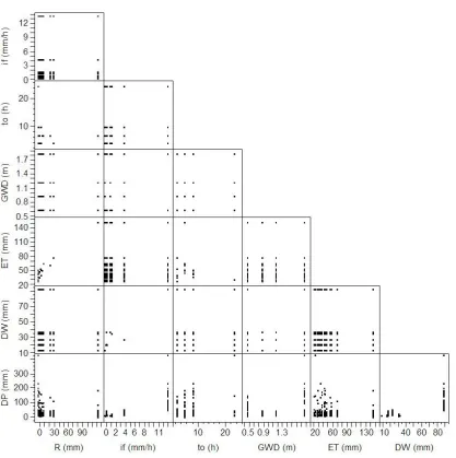
The experimental data set is presented in Figure 4, which visualizes basic relationships in the collected lysimeter data. Note that substantial rainfall (126 mm) between the first and the second irrigation event resulted in high DP measurements for lysimeters with sandy soils. For the remainder of the irrigation season, rainfall was small compared to irrigation and thus did not have much impact on DP.
INSERT FIGURE 4 NEAR HERE
Conceptual model of deep percolation
Bethune et al. (2008) developed a conceptual model of deep percolation based on the data from the lysimeter experiment. The conceptual model of DP is given by:
+
=
055
.
0
tanh
GWD
GWD
i
ET
DW
a
t
i
DP
NSSP f SSP o f
, (2)where SSP and NSSP denote steady-state and non-steady-state percolation, respectively; ET is evapotranspiration and a is an empirical coefficient describing the time-constant percolation rate during redistribution. The term if to represents the percolation during irrigation (when irrigation
water is ponding on the soil surface) assuming steady-state conditions. The ratio DW/ET
denotes the time required for evapotranspiration to utilize DW. Both SSP and NSSP are affected by a factor representing the water table influence:
(
)
=
055
.
0
tanh
GWD
GWD
GWD
f
, (3)where GWD0 is defined as the half depth of water table influence (analogous to the half-life
concept in radioactive decay), i.e., when GWD=GWD0, the reduction factor f is tanh (0.55),
Bethune et al. (2008) found, using the conceptual model, that steady-state percolation during irrigation was the dominant process contributing to deep percolation on most of the studied soils. Non-steady-state percolation (redistribution) was also important for some soil types.
The conceptual model had a root mean square error (RMSE) of 10.9 mm in fitting DP measured in the lysimeter experiment.
The structure of the conceptual model was evaluated using the results from the GP analysis.
GP analysis
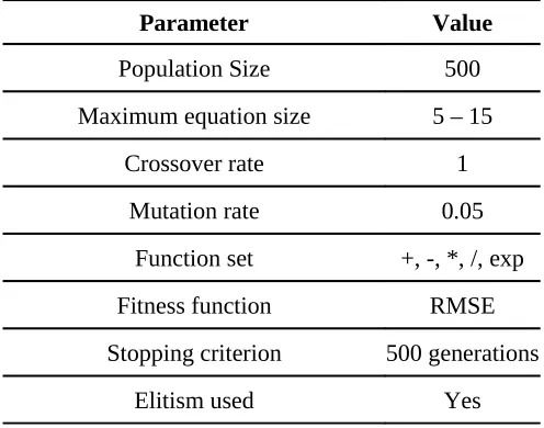
The GP tool software used in this study was GPKernel developed at Danish Hydraulic Institute by Babovic and Keijzer (2000). The GPKernel parameters used for all the GP runs in this study are presented in Table 1. Optimum values for various control parameters were obtained using a trial-and-error process with the objective to minimise the RMSE during the model fitting process.
INSERT TABLE 1 NEAR HERE
As discussed previously, high crossover rates and low mutation rates are usually used. A crossover rate of 1.0 and mutation rate of 0.05 is used in this study and similar values have been used in various applications of GP in water resources (Babovic and Keijzer, 2000; Khu et al., 2001; Muttil and Lee, 2005 and Muttil and Chau, 2006). The terminal set consists of the six input variables {if, to, GWD, DW, ET, R} and DP is the target variable. Along with the simple
math operators {+, -, *, /}, the exponential function {exp} is also included in the function set as
( )
(
exp
2
1
)
/
(
exp
( )
2
1
)
)
tanh(
x
=
x
−
x
+
was used to formulate the conceptual model of DP.The fitness function that was minimised was the RMSE. Performance of evolved GP models was evaluated using the model efficiency ME (Nash and Sutcliffe, 1970), the average error AE and the RMSE which are given by:
∑
∑
= =−
−
−
=
450 1 2 450 1 2)
(
)
(
1
i obs obs i sim obsDP
DP
DP
DP
ME
, (4)∑
=−
=
450 1)
(
450
1
i obs sim
DP
DP
AE
, (5)∑
=−
=
450 1 2)
(
450
1
i obs sim
DP
DP
where DPobs , DPsim and
DP
obs are the observed, simulated and average observed deeppercolation, respectively. In this study, neither a cross-validation of the GP models nor the use of more sophisticated measures of model fitness penalising over-parameterization (such as 'Akaike information criterion') were attempted as the evolved models were very simple with predominantly one and no more than two empirical coefficients to be estimated from the experimental data. Therefore, over-fitting, over-parameterization and poor parameter identifiability were less of an issue.
Interpreting GP models
GP generates simple expressions which can be analysed to provide additional insights into the problem at hand and assist interpretation of the underlying, dominant processes. However, GP has the tendency to evolve uncontrollably large parse trees (called bloating), which lead to incomprehensible models. Thus, to evolve simple and interpretable models, it is necessary to control bloating of GP models. Several techniques for control of bloat have been proposed (Silva and Costa, 2004) and in this study, a limit on the GP equation size (or parse tree size) was used. GP models were evolved using five different values of maximum equation size, namely 5, 8, 9, 10 and 15. For each of these equation sizes, 30 GP models were evolved using different initialisations. The 30 GP runs took approximately 1.5 - 2 hours on an Intel dual core 1.86 GHz PC with 2 GB RAM.
3. Results
Analysis of lysimeter data using GP
Using the five different maximum equation sizes (i.e., 5, 8, 9, 10 and 15) and multiple GP runs with different initialisations, we found that the final infiltration rate of the subsoil if, the ponding
time to and the water table depth GWD were selected at least once per GP run (Table 2). The
amount of water stored in the rootzone between saturation and field capacity DW, the daily average rainfall R and the sum of daily crop evapotranspiration ET between two consecutive irrigations were less frequently (less than once per GP run) selected than if, to, and GWD.
INSERT TABLE 2 NEAR HERE
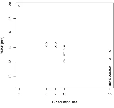
The number of GP models evolved in 30 GP runs increased with maximum equation size. Similarly, as maximum equation size increased, recurrence of GP models diminished and variability in both RMSE and ME increased (Figure 5). No consistent trend was observed for AE.
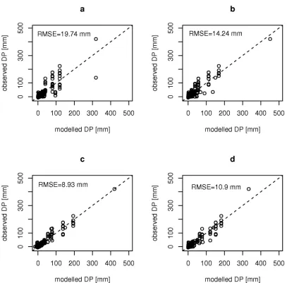
Model performance (in terms of ME and RMSE) tended to improve with increasing equation size (Table 3). For all DP models, variation from the 1:1 line in a plot of model simulations against observations increased as modelled DP increased (Figure 6). This phenomenon, which is common in hydrological data sets, can be due to increasing measurement error in the DP data, or due an inability of the models to predict larger values with the same precision as it does for smaller values. If model prediction error remains unrelated to input variables, and cannot be distinguished from measurement error, it does not preclude the model from giving useful insights into dominant processes.
INSERT TABLE 3 NEAR HERE
INSERT FIGURE 6 NEAR HERE
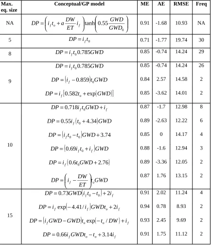
For maximum equation sizes of up to 9, models formulated by GP for different GP runs were very recurrent (Table 3). The GP model DP = if to 0.785GWD was 29 and 26 times
generated in 30 GP runs for the maximum equation size of 8 and 9, respectively. The GP model
DP = ifto 0.785GWD was similar to the conceptual model of steady-state percolation including
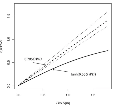
the watertable influence (Equation 2). Only the factor representing the watertable influence is slightly different, i.e. both functions are monotonically increasing as water table depths increase, but at a slightly different rate (Figure 7). Note that the factor representing the watertable influence for the GP model was consistently larger than the factor in the conceptual model, with increasing differences for deeper water tables. These differences occurred because, in contrast to the conceptual model, the GP model does not represent non-steady state percolation during redistribution. For the conceptual model, percolation during redistribution increases for deeper watertables due to decreasing capillary rise. Residuals of the GP model DP
= if to 0.785GWD did not show much noticeable correlation with both model inputs and
variables that were not included into this model (Figure 8).
INSERT FIGURE 7 NEAR HERE
INSERT FIGURE 8 NEAR HERE
Although recurrence in multiple GP runs was lost for larger equation sizes, some of the larger equations were remarkably simple (Table 3). An example of a simple GP model is presented in Equation (7), which was evolved by GP for a maximum equation size of 15. Note that this model has only four inputs and has no coefficients to be estimated from the experimental data:
(
i
fGWD
GWD
)
t
o(
t
oDW
)
i
fDP
=
−
exp
−
/
+
(7)increases as if, GWD, t0 and DW increase. However, for small values of DW, t0 will have convex
parabolic, physically unreasonable relationship with DP, i.e. DP only increases up to a certain value of t0 and then decreases with increasing t0. In contrast to Equation (7), the general trend of
relationships for GP model DP = if to 0.785GWD is physically meaningful even outside the
range of the observed data.
Evaluating conceptual model of deep percolation
For all GP equation sizes, the final infiltration rate of the subsoil if, the ponding time to and the
water table depth GWD were at least once selected per GP run. Up to an equation size of 9, one particular GP model was recurrently evolved in all the 30 GP runs. This GP model contained only the three key variables if, to, and GWD that were related as DP = ifto 0.785GWD. Residuals
of this model did not show much noticeable correlation with both model inputs and variables that were not included into this model. Although GP models with larger maximum equation sizes had better RMSE than the model DP = ifto 0.785GWD, these models were not recurrently
evolved for multiple GP runs and interpretation was difficult due to their complexity. The GP model DP = if to 0.785GWD was similar to the conceptual model of steady-state percolation
including the watertable influence. Based on all these results, steady-state percolation during irrigation as represented by the conceptual model is supported as the dominant process contributing to DP in the lysimeter experiment.
Unlike if, to and GWD, the amount of water stored in the rootzone between saturation
and field capacity DW, which was a key variable representing non-steady-state percolation in the conceptual model, was selected very few times in the multiple GP runs for all equation sizes. In contrast to the conceptual model, the GP model DP = ifto 0.785GWD did not account
for percolation during redistribution. For this GP model, DP was on average only 0.74 mm underestimated. So, no obvious bias was introduced by not representing percolation during redistribution. Furthermore, residuals of this GP model did not show much noticeable correlation with model inputs and variables that were not included into this model. These results indicate that, from the lysimeter data set, non-steady-state percolation can be considered a minor process contributing to DP.
4. Concluding Remarks
As maximum equation size for GP increased, model recurrence was reduced, and model complexity and variability in model performances increased, making interpretation of GP model more difficult and less reliable. For a maximum equation size of 15, GP generated 11 different models. Some of these models had slightly better RMSE than the conceptual model. One of these models (presented in Equation 7) was remarkably elegant, with less inputs than the conceptual model (only if, to, DW and
GWD) and with no coefficients to be estimated from the experimental data, whereas the conceptual model had two empirical coefficients (i.e. a and GWD0). It was initially
believed that this model could provide alternative model formulations to the conceptual model or that it may contain information on additional important processes. However, physical interpretation of the model was found to be reliable only within the range of the observed experimental data. Outside the range of observed data, the model was not physically meaningful and thus reliable physical interpretation of this model or its model components may not be possible. Therefore, GP should only be used with caution and some understanding of the system, as it is easy to over-fit and over-interpret particular features of the data.
Acknowledgements
References
Babovic, V. , Keijzer, M., 2000. Genetic programming as a model induction engine. Journal of
Hydroinformatics 2 (1), 35-60.
Bethune, M. G., Selle, B., Wang, Q. J., 2008. Understanding and predicting deep percolation
under surface irrigation. Water Resources Research 44, W12430, doi:10.1029/2007WR006380.
Beven, K., 2001. How far can we go in distributed hydrological modelling?. Hydrology and
Earth System Sciences 5 (1), 1-12.
Beven, K, Freer, J., 2001. Equifinality, data assimilation, and uncertainty estimation in
mechanistic modelling of complex environmental systems using the GLUE methodology.
Journal of Hydrology 249 (1-4), 11-29.
Breiman, L., 2001. Statistical modelling: the two cultures. Statistical Science 16, 199-231.
Chatfield, C., 1995. Model Uncertainty, Data Mining and Statistical Inference Export. Journal
of the Royal Statistical Society, Series A (Statistics in Society) 158 ( 3), 419-466.
Gaur, S., Deo, M.C., 2008. Real-time wave forecasting using genetic programming. Ocean
Engineering 35 (11-12), 1166-1172.
Holland, J. H., 1975. Adaptation in natural and artificial systems. University of Michigan Press,
Ann Arbor.
Khu, S.T., Liong S.Y., Babovic, V., Madsen, H., Muttil, N., 2001. Genetic programming and its
application in real-time runoff forecasting. Journal of American Water Resources Association
37 (2), 439-451.
Kirchner, J.W., Hooper, R.P., Kendall, C., Neal, C., Leavesley, G., 1996. Testing and validating
environmental models. Science of the Total Environment 183, 33-47.
Koza, J., 1992. Genetic programming: On the programming of computers by natural selection.
MIT Press, Cambridge, MA.
Ljung, L., 1999. System identication. Theory for the user. 2nd edition, Prentice Hall, Upper
Muttil, N., Chau, K. W., 2006. Neural network and genetic programming for modelling coastal
algal blooms. International Journal of Environment and Pollution 28 (3-4), 223-238.
Muttil, N., Lee, J. H. W., 2005. Genetic programming for analysis and real-time prediction of
coastal algal blooms. Ecological Modelling 189 (3-4), 363-376.
Nash, J. E., Sutcliffe, J. V., 1970. River flow forecasting through conceptual models part I - A
discussion of principles. Journal of Hydrology 10 (3), 282-290.
Parasuraman, K., Elshorbagy, A., Si, B.C., 2007. Estimating saturated hydraulic conductivity
using genetic programming. Soil Science Society of America Journal 71 (6), 1676-1684.
Parasuraman, K. , Elshorbagy, A., 2008. Toward improving the reliability of hydrologic
prediction: Model structure uncertainty and its quantification using ensemble-based genetic
programming framework. Water Resources Research 44, W12406,
doi:10.1029/2007WR006451.
Silva, S., Costa, E., 2004. Dynamic limits for bloat control. In: Proceedings of GECCO 2004, K.
Deb et al. (Eds.), 666–677, Springer, Berlin.
Sivakumar, B., 2008. Dominant processes concept, model simplification and classification
framework in catchment hydrology. Journal Stochastic Environmental Research and Risk
Assessment 22, 737-748.
Sivapragasam, C., Maheswaran, R., Venkatesh, V., 2008. Genetic programming approach for
flood routing in natural channels. Hydrological Processes 22 (5) 623-628.
Venables, W.N., Ripley, B.D., 2003. Modern Applied Statistics with S. Springer, New York.
Whigham, P. A., Crapper, P. F., 2001. Modelling rainfall-runoff relationships using genetic
programming. Mathematical and Computer Modelling 33 (6-7), 707-721.
Young, P.C., 2003. Top-down and data-based mechanistic modelling of rainfall-flow dynamics
Figure Captions
Figure 1. Example of GP parse tree representing the GP model f(x) = 2 * exp(-0.5 * x) - 0.6.
Function set nodes are represented by circles and the terminal set nodes by rectangles.
Figure 2. Crossover operator in GP.
Figure 3. Mutation operator in GP.
Figure 4. Scatter plot of experimental data set: DP, deep percolation between two consecutive
irrigations; R, daily average rainfall between two consecutive irrigations; if, final infiltration
rate of the subsoil; to, ponding time; GWD, water table depth of lysimeter; ET, sum of daily
crop evapotranspiration between two consecutive irrigations; DW, soil water stored in the
rootzone between saturation and field capacity.
Figure 5. Root mean square error (RMSE) for 30 GP runs with different maximum equation
sizes.
Figure 6. Modelled vs. observed deep percolations (DP) for selected GP models (a, b, c) and
conceptual model (d; Equation 2, with GWD0=1 m). a)
DP
=
i
ft
0; b)DP
=
i
ft
00
.
785
GWD
;and c)
DP
=
i
fexp
(
−
4
.
41
/
i
f)
GWDt
o+
2
i
f . Dashed line is 1:1 line.Figure 7. Factor representing watertable influence f(GWD) vs. water table depth GWD for GP
model
DP
=
i
ft
00
.
785
GWD
and conceptual model (Equation 3, with GWD0 = 1 m). Dottedlines represent the bootstrap 95% confidence interval for the empirical coefficient of GP model.
Figure 8. Standardised model residuals vs. input variables and variables not included in GP
model
DP
=
i
ft
00
.
785
GWD
. if, final infiltration rate of the subsoil; to, ponding time; GWD,water table depth of lysimeter; DW, soil water stored in the rootzone between saturation and
field capacity; ET, sum of daily crop evapotranspiration between two consecutive irrigations; R,
systematic deviation of residuals from zero, by locally-weighted polynomial regression
Tables
Table 1. Values of control parameters used in GP runs. RMSE is root mean square error.
Parameter Value
Population Size 500
Maximum equation size 5 – 15
Crossover rate 1
Mutation rate 0.05
Function set +, -, *, /, exp
Fitness function RMSE
Stopping criterion 500 generations
Table 2. Input variable counts from 30 GP runs using different maximum equation sizes.
Maximum
Equation size R if to GWD ET DW
5 0 30 30 0 0 0
8 0 30 30 30 0 0
9 0 30 30 30 0 0
10 0 42 36 30 2 2
15 0 84 48 38 0 6
R – daily average rainfall between two consecutive irrigations if - final infiltration rate of the subsoil
to - ponding time
GWD - water table depth of lysimeter
Table 3. Conceptual model and GP models that were evolved more than once in 30 GP runs for
different maximum equation sizes.
Max. eq. size
Conceptual/GP model ME AE RMSE Freq
NA
+
=
055
.
0
tanh
GWD
GWD
i
ET
DW
a
t
i
DP
f o f 0.91 -1.68 10.93 NA5
DP
=
i
ft
0 0.71 -1.77 19.74 308
DP
=
i
ft
00
.
785
GWD
0.85 -0.74 14.24 299
GWD
t
i
DP
=
f 00
.
785
0.85 -0.74 14.24 26(
i
)
t
GWD
DP
=
f−
0
.
859
0 0.84 2.57 14.58 2(
)
[
t
GWD
]
i
DP
=
f0
.
582
o+
exp
0.85 -3.62 14.01 210
f
f
t
GWD
i
i
DP
=
0
.
718
0+
0.87 -1.7 12.98 8(
t
)
GWD
i
DP
=
0
.
55
f 0+
4
.
34
0.89 -2.63 12.22 6(
0−
0)
+
3
.
74
=
i
t
t
GWD
DP
f 0.85 0 14.17 4(
i
t
i
)
GWD
DP
=
0
.
69
f 0+
f 0.88 -1.6 12.94 3(
0
.
6
0+
2
.
76
)
=
i
t
GWD
DP
f 0.89 -3.36 12.05 2GWD
t
ET
DW
i
DP
f
o
−
=
0.87 1.76 13.15 215
(
i
ft
t
)
i
fGWD
DP
=
0
.
73
0−
0+
2
0.91 2.02 11.24 4(
f)
o ff
i
GWDt
i
i
DP
=
exp
−
4
.
41
/
+
2
0.94 0.78 8.93 2(
i
fGWD
GWD
)
t
o(
t
oDW
)
i
fDP
=
−
exp
−
/
+
0.93 2.45 9.69 2f o
o
f
GWDt
t
i
i
DP
=
0
.
66
−
+
3
.
14
0.91 1.75 11.12 2ME - modelling efficiency (Nash and Sutcliffe, 1970)
AE - average error (mm)
RMSE - root mean square error (mm)
Figure 1. Example of GP parse tree representing the GP model f(x) = 2 * exp(-0.5 * x) - 0.6.
Function set nodes are represented by circles and the terminal set nodes by rectangles. 2.0
*
-x -0.5
* 0.6
exp
( )
x z x(
x z)
zf , =0.9* + + * f(x,y,z)=x+
(
0.2*x) (
/ z−y)
(a) Parents z y z x z y x
f( , , )=0.9* +( − )* f(x,z)=x+(0.2*x)/(x+z)
(b) Children
(a) Parent (b) Child
Figure 3. Mutation operator in GP.
(
x y z)
x(
x) (
z y)
f , , = + 0.2* / − f
(
x,y,z)
=x+(
0.2*x)
/y*(
z−x)
-0.2
*
x x
+ /
y
z
*
0.2
*
x x
+ /
y
x
Figure 4. Scatter plot of experimental data set: DP, deep percolation between two consecutive
irrigations; R, daily average rainfall between two consecutive irrigations; if, final infiltration
rate of the subsoil; to, ponding time; GWD, water table depth of lysimeter; ET, sum of daily
crop evapotranspiration between two consecutive irrigations; DW, soil water stored in the
Figure 5. Root mean square error (RMSE) for 30 GP runs with different maximum equation
Figure 6. Modelled vs. observed deep percolations (DP) for selected GP models (a, b, c) and
conceptual model (d; Equation 2, with GWD0=1 m). a)
DP
=
i
ft
0; b)DP
=
i
ft
00
.
785
GWD
;Figure 7. Factor representing watertable influence f(GWD) vs. water table depth GWD for GP
model
DP
=
i
ft
00
.
785
GWD
and conceptual model (Equation 3, with GWD0 = 1 m). DottedFigure 8. Standardised model residuals vs. input variables and variables not included in GP
model
DP
=
i
ft
00
.
785
GWD
. if, final infiltration rate of the subsoil; to, ponding time; GWD,water table depth of lysimeter; DW, soil water stored in the rootzone between saturation and
field capacity; ET, sum of daily crop evapotranspiration between two consecutive irrigations; R,
daily average rainfall between two consecutive irrigations. Dotted lines show (or fail to show)
systematic deviation of residuals from zero, by locally-weighted polynomial regression