Privacy Loss Classes: The Central Limit Theorem in Differential Privacy

(1)

Privacy Loss Classes:

The Central Limit Theorem in Differential Privacy

David M. Sommer

ETH Zurich

Sebastian Meiser

UCL

Esfandiar Mohammadi

ETH Zurich

August 12, 2020

Abstract

(2)

List of Theorems and Corollaries

1 Theorem (Composition) . . . 9

2 Theorem (Equivalence of ADP, RDP and PLD) . . . 20

2.1 Corollary (Equivalence with distinguishing events) . . . 21

3 Theorem (Markov-ADP bound) . . . 21

4 Theorem (The Central Limit Theorem for ADP) . . . 24

5 Theorem (Tight ADP for the Gauss Mechanism) . . . 29

5.1 Corollary (Tight PDP for the Gauss Mechanism) . . . 29

5.2 Corollary (Optimalσfor Gauss-Mechanism PDP) . . . 30

6 Theorem (ADP under composition) . . . 31

List of Lemmas

1 Lemma (Basic Properties of PLD) . . . 9

2 Lemma (Meaning Dual PLD) . . . 12

3 Lemma (Mechanism for Inner Distribution) . . . 12

4 Lemma (Bound Conversion) . . . 13

5 Lemma (δ∗(ε) equals tight-ADP) . . . 14

6 Lemma (Equivalence of ADP and PLD) . . . 16

7 Lemma (Connection to PDP) . . . 17

8 Lemma (Equivalence of PLD and RDP) . . . 18

9 Lemma (Lebesgue-Generalization) . . . 26

10 Lemma (Density Transformation) . . . 27

11 Lemma (PLD of Gauss Mechanism) . . . 27

12 Lemma (Tight ADP for Gauss PLD) . . . 28

13 Lemma (Berry-Esseen and Nagaev Bound,[23]) . . . 31

List of Definitions

1 Definition (Privacy Loss Random Variable) . . . 8

2 Definition (Privacy Loss Distribution (PLD)) . . . 8

3 Definition (Dual PLD) . . . 11

4 Definition (Inner Distribution) . . . 12

5 Definition (ADP) . . . 13

6 Definition (δ∗_{(ε) from PLD) . . . 14}

7 Definition (PDP) . . . 17

8 Definition (R´enyi Divergence & RDP) . . . 18

9 Definition (Concentrated differential privacy) . . . 18

(4)

1 Introduction

Privacy-preservation of personal data is an increasingly important design goal of data processing sys-tems, in particular with recently enacted strong privacy regulations [24]. Modern syssys-tems, however, are increasingly reliant on personal data to provide the expected utility. Hence, privacy and utility are often diametrical, rendering perfect solutions impossible but leaving space for solutions that provide privacy under limited usage.

To quantify the privacy of a mechanism, Dwork et al. [10] proposed a strong privacy notion, called (ε, δ)-approximate differential privacy (ADP). By now, there is a rich literature on ADP guarantees (e.g., [27, 13]). These privacy guarantees naturally deteriorate under repeated adversarial observation, i.e., continued usage increases (ε, δ) to a point where using the mechanism is considered insecure. A tight assessment of this deterioration is essential since loose bounds can lead to underestimating how often a mechanism can be used or to using too much noise. Finding tight bounds is a challenging task and has inspired a rich body of work [16, 2, 8, 12, 21, 20, 26].

The literature contains adaptive sequential composition bounds [26, 16] that aremechanism-oblivious

in the following sense: given a sequence of ADP parameters (εi, δi)i, the adversary may in roundj adap-tively choose any mechanism that satisfies (εj, δj)-ADP. It has been shown [16, 22] that analyzing the approximate randomized response (ARR) mechanism, i.e., analyzing two worst-case (output) distribu-tions parametric solely in a (εj, δj) pair, exactly yields optimal mechanism-oblivious bounds. These results have been used [27] to analyze a mechanism by deriving (ε, δ) before composition and then computing an adaptive composition bound.

Often we are interested in quantifying the privacy of a particular mechanism under composition instead of the privacy of adversarially chosen mechanisms. Recent results show that better fitting worst-case distributions can lead to significantly tighter bounds under composition (Concentrated DP [8, 12], moments accountant & R´enyi DP [2, 21], and Privacy Buckets [20]).

These methods started to more intensely use theprivacy lossof a mechanism that has been proposed by a seminal work by Dinur and Nissim [9]. Most of these approaches, however, introduced novel privacy notions derived from characterizing the moments of the privacy loss (CDP, MA, RDP) and only derived loose bounds for well-established privacy notions, such as ADP. A notable exception is the iterative and numerical PB approach that can fall prey to numerical errors, memory limitations, and discretization problems.

1.1 Contribution

This work directly leverages the privacy loss [9] by constructing a probability distribution out of it, the

privacy loss distribution (PLD). The PLD is similar to the privacy loss random variable used by Dwork and Rothblum [12], but we also consider corner cases where the loss becomes infinite. Our analysis of the PLD, particularly under sequential composition of the mechanism it resulted from, deepens our understanding of privacy-deterioration under composition and yields a list of foundational and practical contributions.

(a) We show that the PLD can be used for deriving the following differential privacy metrics: pure dif-ferential privacy (DP), approximate difdif-ferential privacy (ADP), concentrated difdif-ferential privacy (CDP), R´enyi differential privacy (RDP), and probabilistic differential privacy (PDP). We show that the PLD is a unique canonical representation for RDP and ADP.

(b) We prove that the PLD of any mechanism evolves under independent non-adaptive sequential composition as a convolution and thus, as an application of the central limit theorem, converges to a Gauss distribution, which we call theprivacy loss class of the mechanism. This Gauss distribution has a variance and mean that directly follows from the variance and mean of the PLD and both values linearly grow under composition. We can extend this insight from non-adaptive composition to some adaptive mechanisms (such as adaptive query-response mechanisms), by finding worst-case distributions and an-alyzing the PLD of these worst-case distributions. The leniency regarding adaptive choices naturally reduces the tightness of the resulting bounds and is not the main focus of this work.

(5)

0 0

event spaceo

Pr

[

o

←

M

(

xi

)]

Laplace Noise

M(x0)

M(x1) ₌

⇒

0 0

y

ω

(

y

)

n= 1 Laplace

Gauss

0 0

y

ω

(

y

)

n= 4 Laplace

Gauss

0 0

y

ω

(

y

)

n= 32 Laplace

Gauss

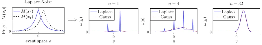
Figure 1: Laplace in Privacy Loss Space for different number of compositions n. Recall that a compo-sition of two independent mechanisms corresponds to a convolution of the privacy loss distribution. As illustration of the privacy loss class and in the spirit of the central limit theorem for differential privacy, a Gauss with identicalµandσ2 _{as the shown privacy loss distribution has been plotted.}

0 0.5 1 1.5 2 2.5 3 3.5 4 4.5 10−8

10−6

10−4

10−2

100

ε

δ

(

ε

)

DP-SGD,n= 216

R´enyi Nagaev Markov Berry-Esseen Gauss Exact

102 ₁₀3 ₁₀4

0.5 1 5 10

n

ε

DP-SGD,δ= 10−4

Nagaev Markov Gauss Exact

Figure 2: Comparing bounds for differentially private stochastic gradient descent mechanism with noise parameter q = 0.01 and σ = 4. Left: after n = 216 _{compositions, right: minimal} _ε _{values over the}

number of compositionsnforδ≤10−4_{. In the right graph, the R´enyi-DP and Berry-Esseen bound did}

not fall into the plotting range and were omitted.

the tightness to invert our formulas, providing analytic (PDP) and numeric (ADP) methods to obtain the smallest standard deviation possible still fulfilling given (, δ)-privacy requirements under n-fold sequential composition; maximizing utility.

(d) Our analysis shows that the Gauss mechanism clearly outperforms the one-dimensional Laplace mechanism under composition in terms of a variance to privacy trade-off: A Gauss mechanism with half the variance as the Laplace mechanism provides the same privacy guarantees, for ADP, PDP and even for (almost) pure DP, except for a tiny delta, which in our example (σ= 40) can be considered negligible even by cryptographic standards: less than 2−80 _{after 128 compositionsand less than 2}−150 _{after 256}

compositions.

(e) We further use the privacy loss class of a given non-adaptive mechanism to prove upper and lower ADP bounds for n-fold sequential composition. We apply the Berry-Esseen and Nagaev normal approximation theorems to the privacy loss class and approximate the PLD afternconvolutions (for n-fold sequential composition). We, thus, pave the way for future research on tight normal approximation bounds for PLDs, which would result in tight bounds forn-fold sequential composition.

(f) We prove that ADP bounds on a differentially private mechanism derived over the PLD can be translated to bound a variation of this mechanism that includes distinguishing events. As an example, we generalize the RDP bounds [2, 21] for the Gauss mechanism to RDP bounds for the truncated Gauss mechanism.

Next, we characterize the PLD under sequential composition (Contribution (b)).

Informal Theorem 4 (The CLT for ADP):LetM be a mechanism andx0, x1be two inputs yielding

the privacy loss distribution ω with finite variance σ2 _{and finite mean}_µ_{. Then, the privacy loss}

distri-butionωn ofM onx0 andx1 afternnon-adaptive sequential compositions has variancen·σ2 and mean

n_·µ. Moreover, if σ2 _>₀ _{and the third absolute moment of} _ω _{is finite, then} _ω

n converges against a

Gauss distribution with variancen_·σ2 _{and mean} _n

(6)

2 Overview

We illustrate a selection of our results to highlight key ideas. Dwork and Rothblum defined theprivacy loss of any observable outcomeoof a mechanismM on inputsx0orx1as the logarithmic ratio between

the probability to observeoon inputx0 compared to on inputx1.

LM(x0)/M(x1)(o) = ln

_{Pr [M}_(x

0) =o]

Pr [M(x1) =o]

.

This privacy loss spans a real-valued random variable obtained by samplingo_∼M(x0) and outputting

LM(x0)/M(x1)(o), which in turn defines the privacy loss distribution (PLD).

2.1 Worst-case distributions

The privacy loss is computed for two distributions, but is not restricted to special cases. For many mechanisms M there are so-called worst-case distributions A and B with a privacy loss maximally as great as that ofM(x0) andM(x1) for all pairs of neighboring inputsx0 andx1. We give some intuition

on how worst-case distributions work and why they typically exist, but refer to Meiser and Mohammadi’s recent work [20] for a more detailed discussion.

For non-adaptive mechanisms, i.e., for mechanisms that do not change structurally from one exe-cution to the next, there is always such a pair of worst-case distributions [11, 2]. In most cases, the worst-case distribution is defined by the worst possible (in terms of privacy) pair of inputs that is still considered neighboring. If mechanisms behave structurally differently on different inputs, the worst-case distributions have to be artificially created by combining the PLDs for all neighboring pairs of inputs, which might be computationally challenging.

Adaptive queries can often be captured as well: queries can be considered part of the input, and they are neighboring if, e.g., without adding noise, the results at most differ by the application-specific sensitivity. As an illustrative example, consider a database-query-response system that adds noise to its real-valued answers to queries q : X → R before releasing them: M(x) := q(x) +N, where N is

a symmetrically distributed random variable with mean zero, e.g., given by the Laplace distribution or the Gauss distribution. If q has a sensitivity of 1, i.e., for all allowed pairs of inputs x0, x1 we

have _|q(x0)−q(x1)| ≤ 1, as is the case for sum-queries, then the distributions obtained by M(0) and

M(1) are worst-case distributions. If a subsequent queryq0 _{differs from}_q_{(potentially depending on the}

mechanism’s output forq), the worst-case distributions remain unchanged, as long as_|q0_(x

0)−q0(x1)| ≤1.

Hence, the results we give for the Gauss mechanism, specifically our analytical formula for differential privacy (Theorem 5), holds in the light of adaptive queries.

For analyzing a mechanism, a pair of worst-case distributions has to exist for M and for all inputs that fall into the neighboring relation. In doing so, we abstract away from the concepts of utility and sensitivity and require the privacy analyst interested in applying our results to provide worst-case distributions. In the remainder of this work we concentrate on a pair of distributionsM(x0) andM(x1)

for a mechanismM :X → U and two concrete inputsx0, x1∈ X. All our results also apply for a pair of

worst-case distributions.

2.2 The privacy loss distribution

Given a pair of distributions, we can consider the corresponding privacy loss distribution. This pri-vacy loss distribution naturally evolves under sequential composition as a convolution of pripri-vacy loss distributions (Theorem 1), as Figure 1 illustrates for the Laplace mechanism. By the central limit the-orem, a privacy loss distribution converges to a predictable Gauss distribution under sufficiently many compositions (Theorem 4).

The privacy loss distribution of the Gauss mechanism also is a Gauss distribution and under convo-lution again remains a Gauss distribution. We give an analytical and efficiently computable formula for ADP and PDP composition bounds for any number of compositions. Note that these are not approximate bounds, but indeed precise characterizations (Theorem 5, Figure 5).

We also provide bounds for arbitrary mechanisms (for which a worst-case reduction exists); after many (n >222_{) compositions, our bounds outperform previous work. Our representation with PLDs}

(7)

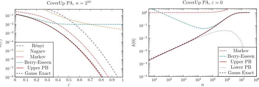
apply normal approximation theorems (the Berry-Esseen Theorem and Nagaev-Bound) to achieve tight bounds for a very large number of observations and very small epsilons, as is, e.g., needed for timing leakage analyses as in CoverUp [25], see Figure 6. The minimum of these normal approximation bounds and the ADP-version of the Markov inequality achieves a very competitive bound, in particular for a very large number of observations. We offer an efficient implementation for computing this minimum.

Figure 2 illustrates our results. The left graph plots for a recent mechanism for training deep neural networks [2] for each εthe minimal δ(ε) such that the mechanism is still (ε,δ(ε))-ADP after 216

com-positions. The right graph shows the minimalεfor whichδ(ε)<10−4_{over the number of compositions}

n. The figure displays the performance of our improved Markov-ADP bound and the performance of our normal approximation bounds, Berry-Esseen and Nagaev. The figure even displays that our exact bound for the Gauss distribution that matches the privacy loss class of the mechanism is very close to the other bounds. Section 6 provides strong evidence that the privacy loss class is actually an accurate characterization of the privacy-preservation of a mechanism and even closer to the tight bounds.

3 Related Work

Vadhan et al. [26] examined the same kind ofn-fold adaptive composition as this work. Roughly speaking, they have shown that privacy will deteriorate as√nε+nε2_{, rather than the (trivial) worst-case}_nε_known

in the literature. Meiser and Mohammadi [20] have recently introduced a novel numerical method for computing ADP bounds, based on a pair of distributions. Their work investigated the privacy loss of mechanisms and approximated this loss to give very good ADP bounds (including lower bounds) under continual observation. Computing their bounds has higher computation requirements, in particular for a very large number n of observations. For the Gauss mechanism our results (Theorem 5) clearly show tighter results for very large n. When repeating their CoverUp analysis, our approach leads to significantly improved results for very highnvalues, which is highly relevant for a system like CoverUp. Kairouz et al. [16] derive tight ADP bounds for the approximate randomized response mechanism (ARR) and use these bounds to prove upper ADP bounds for any mechanism. Their work characterizes set of bounds for the ARR mechanism that contains the tight bounds. This results in a non-trivial optimization problem to find the minimal bounds in this set of bounds. We derive a formula (Example 1) for the ARR under sequential composition that directly computes such minimal bounds.

Recent work on concentrated differential privacy (CDP) [12, 8] directly focuses on the privacy loss for deriving tighter ADP and PDP bounds. This line of work provides interesting insights into differential privacy and into improved bounds for the Gauss mechanism; for other mechanisms, however, these results either provide very loose bounds (e.g., the truncated Laplace mechanism) or no bounds at all (e.g., [2]). Our work, in contrast, identifies the variance, the mean, and the mass of the distinguishing events of the privacy loss distribution before composition (the privacy loss class) as a valuable characterization for the degree of privacy that a mechanism provides. We illustrate that this characterization is accurate and derive upper and lower ADP and PDP bounds.

R´enyi differential privacy (RDP) [21] is a privacy notion based on the log normalized-moments of the privacy loss distribution (the R´enyi divergence). RDP is a generalization of the moments account bound (MA) [2]. We evaluate MA in Section 6 and show an equivalence between RDP’s moments, the PLD, and ADP (Theorem 2), which exceeds the RDP to ADP bound in [21].

In a concurrent work, Balle et al. [5] revisited the Gauss mechanism for optimal denoising in differ-ential privacy. Interestingly, their concurrent work results in the same exact ADP-bound of the Gauss mechanism, without any composition results, however. Additionally, Balle et al. [4] leveraged the char-acterization of differential privacy as an f-divergence to achieve privacy amplification by subsampling. They concurrently proved that ADP bounds imply RDP bounds but not the converse direction. Wang et al. [28] applied similar ideas to R´enyi-DP.

4 Privacy Loss Space

(8)

M(x0), random variable of a probabilistic mechanism

ap-M(x1) plied to inputx0 andx1, often abbreviated asAandB

Pr [o_←A] probability ofo inA

X set of mechanism-inputs

U universe of the mechanisms’ the atomic events

o atomic event in_U

LA/B(o) privacy loss of observationoofA overB

ω privacy loss distribution (PLD)

y privacy loss (i.e., atomic event) in the PLD ω(y) privacy loss pdf/pmf fory

Y set of atomic events in the PLD, the image ofLA/B(U) ω , ω (y), Y dual PLD ofω (Definition 3)

Table 1: Notation table

We further prove that a sequential composition translates to convolution of the respective privacy loss distributions (Theorem 1).

Notation. See Table 1 for a summary of our notation. Formally,a probabilistic mechanism M fromX

toY describes functionM :X_→(Ω_→Y), with Ω :=S

x∈XΩxand Ωxbeing the set of measurable sets on which the random variableM(x) (forx_∈X) is defined.

4.1 Privacy Loss Variables / Distributions

At the core of this work lies the representation of privacy leakage as the privacy loss. The privacy loss L of any one output of the mechanism with respect to two potential inputs is the logarithmic ratio between the probabilities to observe the output for each input. This ratio is of course not defined if this probability is 0 for either the nominator or the denominator. For a more uniform treatment of realistic mechanisms, we introduce distinct symbols∞and−∞that behave similar to infinity and minus infinity. If the nominator is 0, we define the privacy loss_Lto be_−∞, and analogously if only the denominator is 0 we define it to be_∞. This captures distinguishing events, which, if observed, reveal which of the two inputs was used.

Definition 1(Privacy Loss Random Variable). Given a probabilistic mechanismM :_{X → U}, let o_{∈ U}

be any potential output of M and let x0, x1 ∈ X be two inputs. We define the privacy loss random

variable of oforx0, x1 as

LM(x0)/M(x1)(o) =

   

  

∞ if Pr [o_←M(x0)]6= 0and Pr [o←M(x1)] = 0

lnPr[_Pr[o_o←_←M_M(₍_xx_1)]0)] if Pr [o_←M(xi)]6= 0 ∀i∈{0,1}

-∞ else,

where we consider_∞ and -_∞to be distinct symbols.

For readability, we write A := M(x0) and B :=M(x1) for the output distributions of M on two

particular inputsx0andx1and then writeLA/B(o) = ln _Pr[_o

←A] Pr[o←B]

for the privacy loss of the observation o.

The privacy loss _L naturally gives rise to a probability distribution over the privacy losses, the privacy loss distribution (PLD), for two given probability distributions A and B. The set of privacy losses _Y := S

o∈U

LA/B(o) are the atomic events of the distribution. The respective probability density/mass function ω of a privacy loss y is defined as the cumulative weight of all observations o in A with privacy loss y: ω(y) := P

{o| LA/B(o)=y, o∈U}Pr [o←A] with y ∈ Y. Formally, the PLD is

the compound probability distribution of the random variable _L. To be able to sum over all events, we require the universe _U to be countable. For continuous distributions we generalize our results to Lebesgue measurable sets (c.f. Section 5.2).

(9)

Y= [ o∈U

LA/B(o) ⊂R

ω(y) =X

{o| LA/B(o)=y, o∈U}

Pr [o_←A] with y_{∈ Y}

The supportY ofω additionally includes the symbol1 _-_∞_: _{supp(ω) :=}_{_y_|_ω_(y)₆_{= 0}_{} ∪ {}_-_∞}_{. We define}

∀y∈R: -∞< y <∞,y+∞=∞,-∞+y=-∞,-∞+∞=-∞.

Next, we prove basic properties about the PLD.

Lemma 1 (Basic Properties of PLD). For two distributions A andB, let _Y and ω(y)be as in Defini-tion 2, we have

1. The set_Y is countable.

2. _∀y_{∈ Y} : ω(y)_≥0

3. P

y∈Y ω(y) = 1

4. ω(_∞) =P

{x|Pr[o←B]=0}Pr [o←A]

5. ω(-∞) = 0

Proof. The proofs directly follow from Definitions 1 and 2.

1. Y is a mapping from the countable setU and is therefore countable as well.

2. Follows from Pr [o_←A]_≥0 _∀o_{∈ U}.

3. P

y∈Yω(y) =

P

o∈UPr [o←A] = 1.

4. Follows by the definition of the privacy loss_L.

5. By definition of_L, o_{∈ U}:

ω(-∞) =P

{o| LA/B(o)=-∞}Pr [o←A]

=P

{o|Pr[o←A]=0}Pr [o←A] = 0

With these properties at hand, we can prove that the privacy loss distribution of a pair of independent product distributionsA_×C vs. B_×D is the same as the convolution of the privacy loss distributions of the pair of single distributions A vs. B and C vs. D. This theorem is vital because sequential composition of non-adaptive mechanisms, translates to the independent product distributions of the respective mechanisms.

Theorem 1(Composition). LetM:_{X → U} andM0_:_X0 _{→ U}0_{be independent probabilistic mechanisms,}

and letx0, x1∈ X andx00, x10 ∈ X0. Let ω be the privacy loss distribution created byM(x0) overM(x1)

with support _Y, and ω0 _by _M0_(x0

0) over M0(x01) with support Y0 respectively. Let ωc with support Yc

be the privacy loss distribution created by M(x0)×M0(x00) over M(x1)×M0(x01) where × denotes the

independent distribution product. Then,ωc can be derived from ω andω0 as follows:

Yc =yc | yc =y+y0 ∀y∈ Y,∀y0 ∈ Y0

So,_∀yc∈ Yc\ {-∞,∞} we have

ωc(yc) = (ω∗ω0)(yc)

= X

{y, y0_|_y₊_y0₌_y

c}

ω(y)_·ω(y0)

ωc(∞) = 1−[1−ω(∞)]·[1−ω0(∞)] ωc(-∞) = 0

whereω_∗ω0 _{is a convolution, and the set}_Y

c is countable.

1_{We are aware that the support of a probability mass function}_ω₍_y_{) is usually defined as the set of}_y_with_ω₍_y₎₆_{= 0.}

(10)

Proof. LetM :X → U andM0:X0 _{→ U}0 _{be two probabilistic mechanisms, let}_x

0, x1∈ X andx00, x01∈

X0_{. For ease of readability we write} _U2 ₌_{U × U}0_{. We put emphasis on the difference between}_M_(x

0)

andM(x1), as well as betweenM0(x00) andM0(x01) respectively, which leads to four different

probability-terms, namely Pr [o←M(x0)], Pr [o←M(x1)], Pr [o0←M0(x00)], and Pr [o0←M0(x01)] all defined on o∈

U, o0_{∈ U}0_{. We split}_U2₌

U × U0 _{into three sets as follows}

U2

+={(o, o0) | ∀(o, o0)∈ U2,∀i∈ {0,1}: Pr [o=M(xi)]6= 0∧Pr [o0 =M0(x0i)]6= 0} U2

0 ={(o, o0) | ∀(o, o0)∈ U2,∀i∈ {0,1}: Pr [o=M(xi)] = 0∧Pr [o0 =M0(x0i)] = 0} U∞2 =U2\(U+2∪ U02) (one to three probabilities are 0)

Obviously, they are pairwise distinct and contain together all elements inU2₌_U2

+∪ U∞2∪ U02. Therefore,

this proof examines these sets separately: first, the setU2

+ (leading to the convolution property), second

U2

∞ ( forω(∞) and partly ω(-∞)), and lastU02 (leftoverω(-∞)).

First, we examine the set U2

+. This will lead to the convolution property for y 6= -∞,∞. As the

tree sets are separated in a way that no event (o, o0_{) in} _U2

+ has a probability of zero, we do not need

to considerωc(∞) or ωc(-∞) in this part. For all events (o, o0)∈ U+2, the privacy loss is additive under

composition: _∀(o, o)_{∈ U}2 +

L(M(x0),M0(x00))/(M(x1),M0(x01))(o, o

0_{) = ln}Pr [(o, o0)←(M(x0), M0(x00))]

Pr [(o, o0₎_←_(M_(x₁_{), M}0_(x0

1))]

= ln _{Pr [o}

←M(x0)]

Pr [o←M(x1)]

Pr [o0_←_M0_(x0

0)]

Pr [o0_←_M0_(x0

1)]

= ln _{Pr [o}

←M(x0)]

Pr [o_←M(x1)]

+ ln

_{Pr [o}₀

←M0_(x

0)]

Pr [o0_←_M0_(x0

1)]

=_LM(x0)/M(x1)(o) +LM0₍_x₁₎_/M0₍_x0

1)(o

0₎

sinceM andM0 are independent. Let us define

Y+=

yc | yc=y+y0 y∈ Y, y0 ∈ Y0, y, y0 6= -∞,∞ .

AsY andY0 are countable, their compositionY+is countable as well. For readability, let us define

Lc(o, o0) :=L(M(x0),M0₍_x0

0))/(M(x1),M0(x01))(o, o

0₎

L(o) :=_LM(x0)/M(x1)(o)

L0(o0) :=_LM0₍_x0

0)/M0(x01)(o

0₎

Withyc∈ Y+

ωc(yc) =

X

{(o,o0₎_{| L}

c(o,o0)=yc}

Pr [(o, o0)←(M(x0), M0(x00))]

= X

{(o,o0₎_{| L}₍_o₎₊_L0₍_o0₎₌_y

c}

Pr [o_←M(x0)]·Pr [o0←M0(x00)]

= X

{(y,y0₎_|_y₊_y0₌_y

c} X

{o| L(o)=y}

Pr [o_←M(x0)]·



 

X

{o0

| L0₍_o0₎₌_y0

}

Pr [o0_←M0(x00)]



 

= X

{(y,y0₎_|_y₊_y0₌_y_c_}

ω(y)_·ω0(y0),

which is a convolution. We have used that the sums considered converge absolutely; thus, the sum-product is a Cauchy sum-product and thereby the last equality is valid. For the second equality, we have used the independence of M and M0. As there are no events (o, o0) in U2

+ for which one of the four

probabilities Pr [o←M(xi)], Pr [o0←M0(xi)] with i∈ {0,1} equals to zero, we do not need to consider ωc(∞) orωc(-∞) here.

(11)

combinations of these four sets fromU2

∞ to defineU⊥2:

U∞={o | Pr [o←M(x1)] = 0,(o, o0)∈ U_∞2}

U∞0 ={o0 | Pr [o0←M0(x01)] = 0,(o, o0)∈ U∞2 }

U+={o | Pr [o←M(x1)]6= 0,(o, o0)∈ U_∞2}

U+0 ={o0 | Pr [o0←M0(x01)]6= 0,(o, o0)∈ U∞2 }

U⊥2 =U∞2 \(U+×U_∞0 )∪(U∞×U+0)∪(U∞×U∞0 )

First, let us argue about ω(-∞): It is always zero as for any corresponding events of M(x0) have

occurrence probability 0 as in Lemma 1. By construction, the sets U+ and U+0 contain all events

o, o0 for which the corresponding Pr [o←M(xi)] 6= 0 and Pr [o0←M0(x0i)] 6= 0 for i ∈ {0,1}. There-fore P

o∈U+Pr [o←M(x0)] = 1−ω(∞) (analogously forM

0_{). Moreover, all the leftover events in} _U2

⊥

have either Pr [o_←M(x0)] = 0 or Pr [o0←M0(x00)] = 0 or both and are captured in the third and

fourth statement. By construction, if and only if (o, o0₎_∈₍_U

+× U_∞0 )∪(U∞× U+0)∪(U∞× U∞0 ), then

Pr [(o, o0₎_←_(M_(x

1), M0(x01))] = 0 and thus the event is withinωc(∞). ωc(∞) =

X

{(o,o0₎_|_Pr_[₍_o,o0₎_←₍_M₍_x₁₎_,M0₍_x0

1))]=0}

Pr [(o, o0)←(M(x0), M0(x00))]

=X

{(o,o0)|Pr[o←M(x1)]·Pr[o0←M0(x01)]=0}

Pr [o_←M(x0)]·Pr [o0←M0(x00)]

=X

(o,o0₎

∈(U+×U∞0 )

Pr [o_←M(x0)]·Pr [o0←M0(x00)]

+X

(o,o0)∈(U∞×U+0)

Pr [o←M(x0)]·Pr [o0←M0(x00)]

+X

(o,o0₎

∈(U∞×U∞0 )

Pr [o←M(x00)]·Pr [o0←M0(x00)]

= [1₋ω(_∞)]ω0(_∞) +ω(_∞)[1₋ω0(_∞)] +ω(_∞)ω0(_∞) = 1₋[1₋ω(_∞)][1₋ω0(_∞)]

where we have separated the infinite sums as before (independence and Cauchy products) and we have usedP

o∈U+Pr [o←M(x0)] = 1−ω(∞) (analogously forM

0_).

For the third setU2

0, the observation that for any (o, o0)∈ U02 the loss function evaluates to -∞, but

any occurrence-probabilities are zero leads to the conclusion that its contribution to any event inωc is 0.

We show _Yc =

yc | yc =y+y0 ∀y∈ Y,∀y0 ∈ Y0 Note that for all events in U_∞2 \ U_⊥2 we can set y =_∞ and for all events in _U2

\(_U2

+∪ U∞2) we can set y = -∞. Together with the addition rules in

Definition 2, it is valid to define _Yc =_Y+∪{-∞,∞}. Again, we neglect the setU_⊥2 and U02 as they do

not contribute to the privacy loss distribution. _Yc is countable as_Y and_Y0 and_{-_∞,_∞}are countable. this concludes the proof.

4.2 Dual Privacy Loss Distribution

The ADP definition is symmetric, but the notion of a privacy loss distribution (PLD) of A over B is inherently asymmetric sinceω(y) is defined by probabilities inA. We show that it is possible to derive the PLD ofB overA, thedual PLD, directly from the PLD ofAoverB.

Definition 3(Dual PLD). Given a probabilistic mechanismM :_{X → U}, for a privacy loss distribution

ω with supportY created byM(x0)overM(x1)(forx0, x1∈X), the dual privacy loss distribution(dual

PLD) ω with support Y is defined as

Y ₌_{_-_y _| _y_{∈ Y}} ω _{(y) =}_ω₍_-_y)_ey

∀y∈ Y ω ₍_∞_{) = 1}₋P

y∈ Y \{-∞,∞} ω (y)

(12)

Lemma 2 (Meaning Dual PLD). Given a probabilistic mechanism M : X → U, for a privacy loss distribution ω created by M(x0) over M(x1), then the PLD created by M(x1) over M(x0) is the dual

PLD ω as defined in Definition 3.

Proof. Let us split_U in three sets

U+={o | LM(x1)/M(x0)(o)∈ Y \ {-∞,∞}, o∈ U}

U∞={o | LM(x1)/M(x0)(o) =∞, o∈ U}

U0={o | LM(x1)/M(x0)(o) = -∞, o∈ U}

Note that the sets_U+,U∞,U0are pairwise distinct andU =U+∪U∞∪U0. We look at each set individually.

First, the set _U+: As for for all events o ∈ U+ neither Pr [o←M(x0)] nor Pr [o←M(x1)] evaluates to

zero, we can use the logarithmic nature of the privacy loss_LM(x0)/M(x1)(o) =−LM(x1)/M(x0)(o) which

gives us Y +={-y | ∀y∈ Y \ {-∞,∞}}. So,∀y∈ Y +

ω _{(y) =} X

{o| LM(x1 )/M(x0 )(o)=y}

Pr [o←M(x1)],

= X

{x| LM(x0 )/M(x1 )(o)=-y}

Pr [o_←M(x0)]·

Pr [x_←M(x1)]

Pr [o_←M(x0)]

= X

{x| LM(x0 )/M(x1 )(o)=-y}

Pr [o_←M(x0)]·eLM(x1 )/M(x0 )(o)

=ω(-y) ey

There are no events inU+which could go into ω (-∞) or ω (∞). Next, we look atU0. We use the fact that

for allo∈ U0, LM(x1)/M(x0)(o) = -∞and thus Pr [o←M(x0)] = 0. In this case, according to Lemma 1:

ω _(-_∞_{) = 0. Next, for the set}_U

∞, we use

ω ₍_∞_{) =} X

o∈U∞

Pr [o←M(x1)]

= X

o∈U\U0,U+

Pr [o_←M(x1)]

= 1− ω (−∞)

| {z }

=0

− X

y∈ Y +

ω _(y)

Finally, note that the support of ω namely Y coincides with Y +_∪{-_∞,_∞}. This concludes the proof.

4.3 Inner Privacy Loss Distribution

Most of the privacy bounds in this work and in the literature do not consider distinguishing events, i.e., ω(_∞) = 0. Hence, these events with _L(o) = _∞ have to be treated differently. We examine the distribution conditioned on excluding such events.

Definition 4 (Inner Distribution). The inner distribution ω¯ of a privacy loss distribution ω is the normalized distribution withoutω(_−∞)andω(_∞). _∀y_{∈ Y \ {}-_∞,_∞}

¯

ω(y) = Pr

y∼ω[y|y6=∞] =

ω(y) 1−ω(∞)

We can define a mechanismM0 _{that leads to the inner distribution directly.}

Lemma 3 (Mechanism for Inner Distribution). Let M : _{X → U} be a probabilistic mechanism and

x0, x1 be inputs with common support O = {o|∀i ∈ {0,1},Pr [o←M(xi)] 6= 0, o ∈ U}, leading to a

privacy loss distribution ω. LetM0

M,O:X → U be a probabilistic mechanism with Pr

o_←M0

M,O(x)

= Pr [o_←M(x)_|o_∈O]. Then, the privacy loss distribution created by M0

M,O(x0) over MM,O0 (x1) is equal

(13)

Proof. Let Y be the support of ω, y ∈ Y \ {-∞,∞}. Note that ∀o ∈ U, Pr

o←MM,O0 (xi) = Pr [o←M(xi)|o∈O]. Note that∀o∈O,LM0

M,O(x0)/M

0

M,O(x1)(o) =LM(x0)/M(x1)(o) andLM(x0)/M(x1)(o)∈ Y \ {-_∞,_∞}. The PLD ofM0

M,O(x0) overMM,O0(x₁) is

ω0(y) = X

o∈L−1

M_M,O0 (x_{0 )}/M_M,O0 (x_{1 )}(y)

Pr

o←MM,O0 (x0)

= X

o∈L−1

M(x_{0 )}/M(x_{1 )}(y)

Pr [o←M(x0)]

Pr [M(x0)∈O]

= 1

1₋Pr [M(x0)∈/ O]

X

o∈L−1

M(x_{0 )}/M(x_{1 )}(y)

Pr [o←M(x0)]

= ω(y) 1−ω(∞) = ¯ω(y).

The following lemma shows that many of the bounds that do not consider distinguishing events can be generalized if the bound is considered to constrain only the inner distribution.

Lemma 4 (Bound Conversion). Let ω be a privacy loss distribution with support _Y. If there exists a bound_B(γ)on the inner distributionω¯for a positive functiong:_{Y →}R and forγ∈ Y \ {-∞,∞}

X

y≥γ

g(y) ¯ω(y) _{≤ B}(γ)

then the bound can be expressed for the full distribution:

X

y≥γ

g(y)ω(y) _≤ ω(_∞) + [1₋ω(_∞)]_B(γ)

withg(_∞) = 1.

Proof. Let the variables be defined as in the lemma. The statement follows immediately from the definition, settingg(_∞) = 1:

X

y≥γ

g(y) ¯ω(y) = 1 1₋ω(_∞)

X

y≥γ, y6=∞

g(y)ω(y)≤ B(γ)

⇐⇒ X

y≥γ, y6=∞

g(y)ω(y)_≤[1₋ω(_∞)]_B(γ)

⇐⇒ X

y≥γ

g(y)ω(y)_≤ω(_∞) + [1₋ω(_∞)]_B(γ)

4.4 Approximate Differential Privacy

We first present the definition from the literature and then prove that our PLD-based definition is equivalent.

Definition 5 (ADP). Let M : _{X → U} be a probabilistic mechanism and x0, x1 ∈ X. We say M is

(ε, δ)-differentially private (or (ε, δ)-ADP) forx0, x1 if we have for all setsS ⊆ U

Pr [M(x0)∈S]≤eεPr [M(x1)∈S] +δ.

We say that δ is tight for ε and x0, x1 if there is no δ0 < δ such that the mechanism is (ε, δ0)-ADP

for x0, x1. We write δ(ε) for this tight δ of an ε. The ADP-graph is defined as (ε, δ(ε))ε∈R. Given a neighboring relation, we call the mechanism M (ε, δ)-ADP if M is (ε, δ)-ADP for all neighboring

(14)

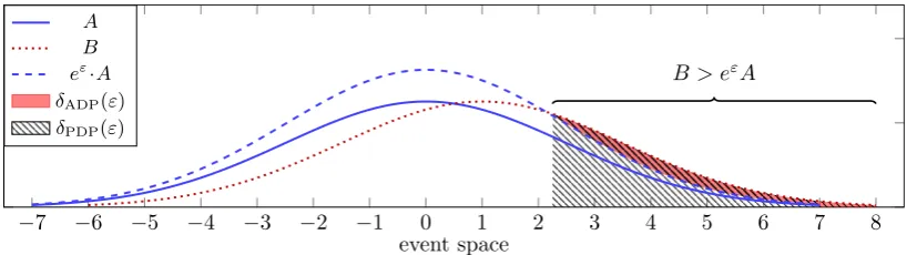
The same definition applies if, instead of talking about mechanisms that were based on data universes X, we consider the timing leakage of an algorithm that is based on a secret key, or if we quantify the difficulty of distinguishing two distributions after a single event. For a illustration of ADP on two probability distributions, see Figure 4, following a depiction in [20].

The privacy loss space directly enables us to compute a tight value δfor every value of εsuch that (ε, δ)-differential privacy is satisfied. This representation is vital for this work. We connect our definition from above to the definition of tight ADP [20].

Definition 6 (δ∗_{(ε) from PLD)}_. _{For a probabilistic mechanism} _M _: _{X → U} _{with inputs} _x

0, x1 ∈ X

creating a privacy loss distributionω with support _Y and forε_≥0 we define

δ∗M(x0),M(x1)(ε) =ω(∞) +

X

y>ε, y∈Y\{-∞,∞}

(1₋eε−y)ω(y)

We now show that Definitions 5 and 6 are equivalent.

Lemma 5 (δ∗_{(ε) equals tight-ADP)}_. _{For every probabilistic mechanism} _M _:_{X → U}_, _x

0, x1 ∈ X, and

for any values ε, δ _≥ 0, M is (ε, δ(ε))-tightly ADP for x0, x1 as in Definition 5 iff we have δ(ε) =

δ∗_M₍_x₀₎_,M₍_x₁₎(ε)(c.f., Definition 6).

Proof. LetM be a probabilistic mechanism andx0, x1∈ X be two inputs. For simplicity, let us denote

A(o) := Pr [o_←M(x0)] andB(o) := Pr [o←M(x1)], and letL−_A/B1 (y) ={o|y=LA/B(o), o∈ U} be the pre-image ofy. First, we show that

X

o∈U

max(0, A(o)−eεB(o)) =ω(∞) +X

y>ε, y∈Y\{-∞,∞}

(1−eε−y)ω(y)

Afterwards, we apply a lemma from prior work to prove the equivalence of the left hand side to tight-ADP. Let us first consider only the term max(0, A(o)−eε_{B(o)): for any}_y_{∈ Y \ {}_-_∞_,_∞}_and_∀_o_{∈ L}−1

A/B(y)

y= lnA(o)

B(o) ⇐⇒ B(o) =e

−y_A(0)

This allows us to re-write

max(0, A(o)₋eεB(o)) = max(0,(1₋eε−y)_·A(o)) = (

[1₋eε−y_]A(o) _if_{y > ε}

0 else

where we have used the fact that _∀o _{∈ U}, A(0)_≥0. After this preparation, we can come to the next step. Keep in mind that the support_Yofω contains all possible outcomes the loss_LA/B(o) can achieve for allo_{∈ U}. Then

X

o∈U

max(0, A(o)₋eεB(o)) = X o∈L−1₍_∞₎

max(0, A(o)₋eεB(o) | {z }

=0

)

+ X

o∈L−1_(-_∞₎

max(0,

=0

z }| {

A(o)₋eεB(o)

| {z }

≤0

)

+ X

y∈Y\{-∞,∞}

X

o∈L−1₍_y₎

max(0,[1₋eε−y]_·A(o))

= X

o∈L−1₍_∞₎

A(o) + X

y>ε,y6=∞

X

o∈L−1₍_y₎

[1₋eε−y]_·A(o)

=ω(∞) + X

y>ε, y∈Y\{-∞,∞}

[1−eε−y]ω(y)

=δ∗M(x0),M(x1)

=:δ∗

where we have used the definition ofω(y) =P

o∈L−1₍_y₎A(o), the fact thateε>0, and∀o∈ U, A(o), B(o)≥

(15)

−

5

0

5

0

event space o

Pr

[

o

←

M

(

xi

)] Uniform noise

0 ∞

0

y

ω

(

y

)

n= 1

0 ∞

0

y

ω

(

y

)

n= 4

⇒

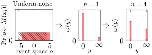
Figure 3: Uniform noise and its privacy loss distribution before composition (n = 1) and after a few compositions (n= 4).

Claim([20, Lemma 1], Connection to tight-ADP). For everyε, two distributionsA andB over a finite universeU are tightly(ε, δ)-ADP with

δ= max P

o∈Umax (Pr [o←A]−eεPr [o←B],0), P

o∈Umax(Pr [o←B]−eεPr [o←A],0)

.

which in application directly concludes the proof.

One immediate corollary is the exact tight-ADP formula for the approximate randomized response mechanism Mε,δ (with parameters ε ≥ 0, δ ∈ [0,1]), shown to be a worst case mechanism [16] for (ε, δ)-ADP.

Example 1 (ARR). Approximate Randomized Response for ξ≥0, 1≥∆≥0, is defined as follows:

Pr [o_←M(x0)] =p0(o),Pr [o←M(x1)] =p1(o) with

p0(o) =

     

    

∆ o= 1

(1−∆)eξ

eξ₊₁ o= 2 (1−∆)

eξ₊₁ o= 3

0 o= 4

p1(o) =

     

    

0 o= 1

(1−∆)

eξ₊₁ o= 2 (1−∆)eξ

eξ₊₁ o= 3

∆ o= 4

Its privacy loss distribution ω can be seen as a shifted binomial distribution, which has a very simple form under convolution. Using Theorem 1 and Lemma 5, forncompositions, we get the exact result

δ(ε) =(1−δ) n

(1 +eξ₎n · n X

k=dkn,εe

_n

k

_h

1₋eε−ξ(2k−n)i_eξ(n−k)

+ [1₋(1₋δ)n]

with_dkn,εe= max[0,min[n,ceil(ε+₂_ξnξ)]]. For a detailed derivation, see Appendix A.1.

Example 2(Non-DP uniform noise). Consider a mechanism that adds uniform noise to its input. We refer to Figure 3 for a graphical depiction. Let M : X _→ U, with U =_{−5, . . . ,5_}, x1, x2 ∈ X, and

Pr [o_←M(x0)] =p0(o),Pr [o←M(x1)] =p1(o)be

p0(o) =

(₁

9 o∈ {−5, ..,4}

0 o= 5 p1(o) =

(

0 o=₋4

1

9 o∈ {−4, ..,5}

leading to

ω(y) = (

8

9 y= 0 1

9 y=∞

The privacy loss distribution ω is not (ε,0)-ADP as _∀ε > 0, ε < _LM(x0)/M(x1)(o=−5) = ∞, i.e.

ω(∞)6= 0, but it is(ε,1₉)-ADP∀ε≥0. Moreover,

ωn(y) = (

(8 9)

n _y_{= 0}

1− 8 9

n

y=∞

(16)

−7 −6 −5 −4 −3 −2 −1 0 1 2 3 4 5 6 7 8 B > eε_A

event space

A B eε

·A δADP(ε) δPDP(ε)

Figure 4: A graphical depiction of the (truncated) Gauss mechanism on two inputs,A=N 0, σ2 , B= N 1, σ2

, and of how to compute ADPδADP(ε) and PDP δPDP(ε) for a given valueε. Note thateε·A

is not a probability distribution.

4.4.1 Equivalence of PLD and ADP-Graphs

We now show that an ADP-graph is as expressive as the privacy loss distribution. For distributions with finite support, it is possible to reconstruct the PLD from the (ε, δ(ε))ε sequence. In practice, finite support is typically the case due to discretization and finite representations of numbers. From Lemma 5, the opposite direction then follows. This is a significant result, as the privacy loss distribution is sufficiently strong for other important privacy notions.

Lemma 6(Equivalence of ADP and PLD). There exists a bijectionRsuch that the following holds. For any probabilistic mechanism M on inputs x0 andx1 with a privacy loss distribution (Y, ω) with finite

cardinality_|Y|=k(fork_∈N), we get the tight ADP-graph(ε, δ(ε))εforx0, x1 (as in Definition 5) with

R(_Y, ω) = (ε, δ(ε))ε and backwards R−1((ε, δ(ε))ε) = (Y, ω).

Proof. To show bijectivity of R, we need to prove injectivy and surjectivity. First, some general con-siderations. According to Definition 5 and Lemma 5, for all mechanisms M : _{X → U} and all inputs x0, x1∈ X,δ(ε) of the tight ADP-graph is of the following form, where (Y, ω) is the PLD ofM(x0) and

M(x1): δ(ε) =P_y>ε,y_∈Y(1−eε−y)ω(y). Moreover, for any PLD and for all y∈ Y, ω(y)>0 and thus

each single summand (1−eε−y₎_ω_{(y) that is included in the sum (i.e.,}_{y > ε) is always positive.} By definition, for all PLDs (Y, ω) generated by all M on all inputsx0, x1, the image of the map

R: (_Y, ω)_→ 

ε, X

y>ε,y∈Y

(1₋eε−y₎_ω(y) 



ε

(1)

contains all valid tight ADP-graphs. Therefore,R is surjective.

We now prove injectivity by contradiction. Assume there are two non-equal PLDs (_Y, ω),(_Y0, ω0₎

for which R outputs the same tight ADP-graph R(_Y, ω) = (ε, δ(ε))ε and R(Y0, ω0) = (ε, δ0(ε))ε with R(_Y, ω) =R(_Y0, ω0_).

If the PLDs consist of a single and identical y, i.e. _Y = _Y0 = _{y_}, from δ(ε) = δ0_{(ε) follows}

immediatelyω(y) =ω0(y) as the term (1₋eε−y_{) is identical in both. This is a contradiction. Otherwise,} if we have more than a single and identical y, we can find the minimal distance between any twoy in Y ∪ Y0: Askis finite andY,Y0 are discrete, the minimal distance isη= miny0,y1∈Y∪Y0,y06=y1|y0−y1|>0.

This means that∀y0, y1∈ Y ∪ Y0 withy06=y1,y1∈/(y0−η, y0).

Letyn = maxy∈Y∪Y0y. We prove the statement by induction. Base step: Asδ0(y_n) =δ(y_n), we get

ω0(∞) = ω(∞) immediately by Definition 6. Induction step: Let yn ∈ Y, otherwise, switch (Y, ω) and (_Y0, ω0_{). If}_y

n ∈ Y/ 0, then∀ε∈(yn−η, yn),δ(ε)−δ0(ε) = (1−eε−yn)ω0(yn)>0. Therefore,δ(ε)6=δ0(ε). This is a contradiction. Ifyn∈ Y0, then letε1=yn−η₂ and

δ0(ε1) = (1−eε1−yn)ω0(yn) + X

y0_>y

n,y0∈Y0

(1−eε1−y0_)ω0_(y0_{) +}_ω0₍_∞₎

δ(ε1) = (1−eε1−yn)ω(yn) + X

y>yn,y∈Y

(17)

But by previous induction steps:

X

y0_>y

n,y0∈Y0

(1₋eε1−y0_)ω0_(y0_{) +}_ω0₍_∞_{) =}X

y>yn,y∈Y

(1₋eε1−y_)ω_{(y) +}_ω₍_∞₎

Therefore, by δ0(ε1) = δ(ε1) ⇒ ω0(yn) = ω(yn) as the term (1−eε1−yn) is identical. Now we define yn−1 = maxy∈Y∪Y0_\{_y

m|m≥n}y and repeat until Y ∪ Y

0_{\ {}_y

m|m≥n} = {}. This will give usY =Y0 and ω0 =ω, which is in contradiction to our assumptions. This proves injectivity. As we have proven injectivity and surjectivity forR, we can conclude bijectivity.

4.5 Probabilistic Differential Privacy

Probabilistic differential privacy [18, 14] is a very intuitive variant of approximate differential privacy (see Figure 4). The main idea is to require that with probability 1-δpureε-differential privacy holds. While this definition has a clear semantics and is easy to understand, it is not closed under post-processing [19], which is a crucial property for practical applications; hence, this work concentrates on ADP. Nevertheless, we show that the privacy loss distribution is sufficient for precisely computing PDP bounds.

Definition 7 (PDP). A probabilistic mechanism M : _{X → U} is (ε, δ)-probabilistically differentially private (PDP) forx0, x1∈ X, whereε≥0andδ≥0, if there are setsS0δ, S1δ ⊆ UwithPr

M(x0)∈S0δ

≤ δ andPr

M(x1)∈S1δ

≤δ, s.t., for all setsS_{⊆ U}, the following in-equations hold:

Pr

M(x0)∈S\S0δ

≤eε_·Pr

M(x1)∈S\S0δ

∧Pr

M(x1)∈S\S1δ

≤eε·Pr

M(x0)∈S\S1δ

. (2)

M is tightly(ε, δ)-PDP forx0, x1 if δis minimal for ε, i.e., if for allδ0 such that M is(ε, δ0)-PDP for

x0, x1,δ0 ≥δ. Given a neighboring relation, ifM is(ε, δ)-PDP for any neighboringx0, x1∈ X then M

is(ε, δ)-PDP.

The conditions of PDP can be directly translated to the privacy loss space as it requires each of tails withy≥εof a PLDω and its dual PLD ω to be smaller thanδ:

Lemma 7 (Connection to PDP). Let M : X → U be a probabilistic mechanism and x0, x1 ∈ X two

inputs with the PLDω and let ω be its dual PLD, then

M is(ε, δ)-PDP forx0, x1⇐⇒

P

y>ε,y∈Yω(y)≤δ

P

y>ε,y∈ Y ω (y)≤δ

Proof. Letω with support_Y be created by M(x0) andM(x1). First, notice that Equation (2) in the

PDP definition is equal to the privacy loss function: fori_{∈ {}0,1_}:

LM(xi)/M(x1−i) S\S δ i

= ln Pr

M(xi)∈S\Siδ

Pr

M(x1−i)∈S\Siδ

≤ε

Let us create two sets

Si0:={o | LM(xi)/M(x1−i)(o)> ε, o∈S δ i}

As S0

i ⊆Siδ ⇒ Pr [M(xi)∈Si0]≤δ. Moreover, ∀o∈Siδ\S0i : LM(xi)/M(x1−i)(o)≤ε by construction.

Therefore,

LM(xi)/M(x1−i)(o)≤ε ∀o∈S\S

0

i= (S\Siδ)∪(Sδi \Si0) (3) which means that allo_∈S with_Li(o)> εare in Si0.

δ≥Pr [M(x0)∈S00]

I

= X

o∈S0

0

Pr [o_←M(x0)]

II

=X

{o| LM(x0 )/M(x1 )(o)>ε, o∈S}

Pr [o←M(x0)]

III

= X

y>ε

(18)

where we have used independence of elementary events (I), Equation (3) (II), and the privacy dis-tribution definition (III). The argument for ω follows analogously. This proves one direction of the lemma. For the other direction, note that we have only used equalities, that Si0 ⊆ Siδ, and that ∀o∈S\Si0,LM(xi)/M(x1−i)(o)≤ε⇒ ∀o∈S\S

δ

i,LM(xi)/M(x1−i)(o)≤ε.

4.6 R´

enyi Differential Privacy & Concentrated Differential Privacy

Recent work introduced novel ADP bounds that are based on the R´enyi divergence (the logarithm of the higher moments of the exponentiated privacy loss random variableeL_{): concentrated DP (CDP) [12, 8],}

Rényi DP (RDP) [21], and the moments accountant [2]. This Rényi divergence can be defined using the PLD. In particular, as CDP and RDP are based on the Rényi divergence, Lemma 6 implies that RDP and CDP can be determined from the tight APD-graph (ε, δ(ε))ε(for distributions with finite support). These bounds were motivated as more comprehensively capturing the privacy guarantees of mechanisms. In fact, the work on concentrated differential privacy can be seen as a direct predecessor of the present work.

The R´enyi divergence of two distributions can be directly derived from their PLD. We begin with defining the R´enyi divergence, then proceed with RDP and then with CDP.

Definition 8 (R´enyi Divergence & RDP). The R´enyi divergence_Dα(M(x0)|M(x1))with α >1 for a

probabilistic mechanismM :_{X → U} and two inputsx0, x1∈ X is defined as

Dα(M(x0)|M(x1)) = 1

α₋1lno∼ME(x1)

eLM(x0 )/M(x1 )(o)

α

D1(M(x0)|M(x1)) = E

o∼M(x0)LM(x0)/M(x1)(o)

R´enyi differential privacy characterizes privacy as the sequence of R´enyi divergences: (α, Dα)α. Given a

neighboring relation,M hasε-R´enyi differential privacy of orderα >1((α,ε)-RDP) if_Dα(M(x0)|M(x1))≤

εfor all neighboringx0, x1∈ X.

Note that _D1(M(x0)|M(x1) coincides with the Kullback-Leibner (KL) divergence from M(x0) to

M(x1). This is a natural property of the PLD, if and only if no output o ∈ U has an infinite privacy

loss. Analogously, we get the KL divergence fromM(x1) overM(x0) by the dual PLD .ω

R´enyi differential privacy can be translated to (ε, δ)-PDP by using a logarithmic version of the Markov bound as follows: whenever (α, Dα)α, then also (ε, αDα−αε)-ADP holds [21]. The moments accountant uses the same characterization and proposes (ε,minα(αDα−αε)) as ADP bounds (as (ε, δ)-PDP implies (ε, δ)-ADP).

CDP requires that the R´enyi divergence be bounded by an affine linear function, which can lead to tighter bounds for some mechanisms (e.g., the Gauss mechanism) but renders CDP unapplicable for other mechanisms (e.g. [2], see Section 6). We use the representation from Bun and Steinke [8], called zero-concentrated DP.

Definition 9 (Concentrated differential privacy). A mechanism M :X → U satisfies (ξ, ρ)-CDP if for allα >0, and all neighboringx0, x1∈ X (for a neighboring relation),Dα(M(x0)|M(x1))≤ξ+ρα.

4.6.1 Equivalence of PLD and RDP

RDP is closely connected to the moments of the privacy loss distribution [28]. In fact, the α-R´enyi-divergenceDαis theα-1-root of the logarithm of the (α-1)-moments of the exponentiated distribution of ω. If the momentsρλ of the exponentiatedωare are not growing too fast,|ρλ|< cdλλ! for aλ >0, then we have equivalence, i.e., we can compute the moments from the privacy loss distribution of a mechanism and vice versa. For privacy loss distributions on a bounded support we always have equivalence.

Lemma 8(Equivalence of PLD and RDP). There exists a bijectionRRDP such that the following holds.

For any probabilistic mechanism M with a countable support on inputs x0 and x1 with a privacy loss

distribution(_Y, ω), s.t.,ω(_∞) = 0, the R´enyi Divergence of orderλwithλ >0of M(x0)andM(x1)is

mλ= 1 λln

E y∼ωe

λy

=Dλ+1(M(x0)|M(x1)) (4)

(19)

Proof. This proof is separated in three parts. First, we show Equation (4). Second, we show that there exists a bijectionR0between R´enyi-DP and the exponentiated PLD (exp-PLD), defined as ({exp(y)|y∈ Y}, ω◦ ln), where (Y, ω) is the PLD of A and B. Third, we show the existence of a bijection R between the exp-PLD and the PLD itself.

First, let us show the equality betweenmλand the R´enyi-DivergenceDα. For simplicity, let us denote A(o) := Pr [o_←M(x0)] and B(o) := Pr [o←M(x1)]. Asω(∞) = 0, there is noo ∈ U where B(o) = 0

andA(x)₆= 0. Therefore, we can do the following:

1 λln

E y∼Ωe

λy

= 1

λln o∼EA

A(o) B(o)

λ!

= 1 λln

X

o∈U

A(o)

_A(o)

B(o) λ

= 1 λln

X

o∈U

B(o)

A(o) B(o)

λ+1

= 1 λlno∼EB

_A(o)

B(o)

λ+1

=_Dλ+1(A|B)

For the second part, the bijection between RDP and exp-PLD, we derive for anyλthe corresponding moment as in the calculation from above. This is an algebraic identity, i.e. any PLDω generated by two distributionsA andB results in one specific R´enyi sequence (α, Dα(A|B))α.

The other directionω◦ln⇐(α, Dα)αis more tricky as there are cases where more than one distribu-tion have the same moments (Hausdorff moments problem). First, let us defineρλ:= exp(λ·mλ)>0 and notice that the conditionρλ < cdλλ! is sufficient such that the power series Pλ>0ρλr

λ

λ! has a positive

convergence radius. More formally, if _∃c, d, d0>0, s.t. 0< ρλ< cdλλ! and d0> d, then∀rwith 0< r <_d10

the power series 0<P λρλr

λ λ! <

P

λcdλλ!r λ λ! < c

P λ dd0

λ

<_∞as 0< d

d0<1 leads to a geometric series.

Now we apply the following claim about probability measures and moments:

Claim([6, Theorem 30.1]).Letµbe probability measure on the line having finite momentsa=R∞

∞ xkµ(dx)

of all orders. If the power series P

kαkrk/k! has a positive radius of convergence, then µ is the only

probability measure with the moments(αi)i∈N.

By this claim, we know that, if the previous power series has a positive convergence radius, then there exists a unique probability measureµfor a given series of moments (Dα(A|B))α. As shown above, the moments of the exp-PLD are exactly the R´enyi divergences; hence, this uniqueness of the measure implies thatµequals the exp-PLD (_Y0, ω_◦ln).

For the third part, we then observe that we can transform any PLD into the exp-PLD (_Y0, ω_◦ln) and vice versa. This is a bijective step, since the exponentiation exp : (-_∞,_∞)_→(0,_∞) is bijective and the logarithm ln : (0,_∞) _→ (-_∞,_∞) is bijective on the domain of strictly positive real values. More precisely, for a probability space (_Y, E, ω) the following function R is bijective, where _Y is the set of atomic events,E := 2Y is the set of all events onY, andω is the probability measure:

R(Y, ω) := ({exp(y)|y∈ Y}

| {z }

=:Y0

, ω◦ln | {z }

=:ω0

)

Next, we will show that, with E0= 2Y0 ={{exp(y)|y∈v} |v∈E}, (Y0, E0, ω0) is a probability space. In particular, we show that in this new probability space,ω◦ln is countably additive: for any countable collection _{E_i}0

i∈I with pairwise disjoint events Ei0 ∈ E0, we know that there are events Ei ∈ E s.t., E0

(20)

follows.

ω0 [ i∈I

E0i !

=ω ln [

i∈I Ei0

!!

=ω (

ln(v0)|v0∈[ i∈I

Ei0 )!

=ω 

  



ln(exp(v))

| {z }

=v

|v_∈[ i∈I

Ei  

 



=ω [

i∈I

{v_|v_∈Ei} !

As _Yis countable andω is countably additive, we can write this as a sum (_∗). Since the setsEi are pairwise disjoint, equality (_∗∗) holds. Plugging in the definition ofω0 _and_E

i, we get the following.

ω [

i∈I

{v_|v_∈Ei} !

(∗)

=X

v∈S

i∈IEi

ω(v)(∗∗=)X i∈I

ω(Ei) = X

i∈I

ω_◦ln(Ei0) = X

i∈I ω0(Ei0)

Hence, we obtain that (_Y0, ω0_{) (together with} _E0 _{= 2}Y0

) is a probability space. Now, we can create a bijectionRRDP. AsR(Y, ω) = (Y0, ω◦ln) andR0(Y0, ω◦ln) = (α, Dα)αare both bijections,RRDP:=R0◦R

is also a bijection andRRDP(Y, ω) =R0(R(Y, ω)) =R0(Y0, ω◦ln) = (α, Dα)α.

4.7 Equivalence of R´

enyi-DP and ADP

From Lemma 6, we know that for any mechanism M and any two inputs x0, x1 the ADP-graph can

be bijectively mapped to the PLD and vice versa, if the common support is discrete and finite. From Lemma 8, we know that for any mechanismM and any two inputsx0, x1the Renyi Divergences can be

bijectively mapped to the PLD and vice versa, as long as the sequence of R´enyi Divergences satisfy a technical sanity condition. As a result, we can conclude that the series of moments (Dα)α, the ADP-graph and the PLD contain the same information and can be transformed into one another.

Theorem 2 (Equivalence of ADP, RDP and PLD). There exists bijectionsRADPand RRDP such that

the following holds. Given a mechanismM. Let(x0, x1)be an arbitrary but fixed pair of inputs such that

• ∀o∈ U, i∈ {0,1},Pr [o←M(xi)]6= 0

• the support _Y of the PLD ofM(x0) andM(x1)has finite cardinality |Y|=k(fork∈N), • the support of M(x0)and of M(x1)is countable, and

• ∀λ >0,_Eo∼M(x0)

h_Pr[_o

←M(x0)] Pr[o←M(x1)]

iλ

< cdλ_λ!_{for two positive constants} _{c, d}_.

Let (ε, δ(ε))ε∈R be the ADP-Graph for x0, x1 (Definition 5), let (α, Dα(M(x0)||M(x1))) be the

R´enyi-Divergence-sequence ([21]), letω be the PLD (Definition 2). Then, the following diagram commutes:

M, x0, x1

PLD

(Y, ω)

RDP

(α, Dα(M(x0)||M(x1)))α∈N ADP

(ε, δ(ε))ε∈R

RRDP

RADP

Proof. Lemma 6 states that there is a bijection RADP such that for all mechanisms and all pairs of

inputs x0, x1 such that the support of the PLD Y has finite cardinality |Y| = k (for k ∈ N) we have

(21)

with the support ofM(x0) and ofM(x1) is countable and exp(λ·|mλ|)< cdλλ! for two positive constants c, dwe haveRRDP((α, Dα(M(x0)||M(x1)))α) =ω. Note that

mλ= 1 λln

E y∼ωe

λy₌ 1 λln

E o∼M(x0)e

λlnPr[o←M(x0 )] Pr[o←M(x_{1 )]}

leads to

E o∼M(x0)

_{Pr [o}

←M(x0)]

Pr [o←M(x1)]

λ

< cdλ_λ!

As both mappings are bijections, the diagram commutes.

The previous result can be extended to mechanisms with non-equal image space, i.e. withω(_∞)₆= 0.

Corollary 2.1(Equivalence with distinguishing events). GivenM on two inputsx0, x1 with

distinguish-ing events and MM,O0 (x)as in Lemma 3, we can apply Theorem 2, resulting in a bijection for the inner

distribution ω¯ of M(x0) over M(x1) (see Definition 4), which allows us to consider the distinguishing

events separately.

Proof. This follows directly from Lemma 3 and Theorem 2.

4.8 Markov-ADP Bound

Next, we refine an ADP bound introduced by the moments accountant [2], which we coinMarkov-ADP

bound. We use Markov’s inequality to limit the privacy loss. In contrast to [2], we discretize the tail and incorporate its contribution in a more fine-grained manner.

Theorem 3 (Markov-ADP bound). A mechanism M : _{X → U} with two inputs x0, x1 ∈ X, and a

privacy loss distributionω with support_Y created byM(x0)overM(x1). LetP be any finite non-empty

sub-set of_Yn, i.e.,P ={y0, . . . , yk} ⊆Rk+1withyi< yi+1∀i. Then, afterncompositions and forε∈ P,

ε < y0,

δ∗_M₍_x₀₎(ε)_{≤ T}(yk) + X

yi≥ε,yi∈P

1₋eε−yi_·_[_T_(y

i)− T(yi−1)]

with

T(y) = min

λ o∼ME(x0)

eλ·ln

_Pr[_o←M(x0 )] Pr[o←M(x1 )]

n

·e−λ·y

is a upper bound for tight-ADP forx0, x1 and smaller or equal to the PDP bound given by RDP [21]. Proof. Letωn generated by A=Mn(x0) and B =Mn(x1) be the distribution ω after nindependent

self-compositions. The beginning of this proof is inspired byTheorem 2of [2] which has already proven

the composability of the log moments

αAn_,Bn(λ)≤ n X

i=0

αA,B(λ) =n·αA,B(λ)

with

αA,B(λ) = ln E o∼Ae

λlnPr[o←A] Pr[o←B]

for allλ >0. Moreover, by applying Markov’s inequality, they have proven for allγ >0, λ >0,

Pr

y∼ω[y≥γ] = X

y≥γ,y∈Yn

ω(y) ≤ exp(αA,B(λ)−λγ)

From which follows forωn and the correspondingYn

X

y≥γ,y∈Yn

ωn(y)≤min

λ>0exp(αAn,Bn(λ)−λγ)

≤min

λ>0exp(n·αA,B(λ)−λγ)

= min λ>0exp

n_·ln_E

o∼A h

eλlnPr[Pr[oo←←AB]]

i −λγ

= min λ>0

Eo∼A h

eλ·lnPr[Pr[oo←←AB]]

in

(22)

as this is valid for allλ, the term can be minimized.

W.l.o.g, we can assumeT(γ) to be monotone decreasing (∀η >0,T(γ)≥ T(γ+η)), else we just set T(γ) =T(γ+η) as a probability mass cannot increase while we reduce the evaluated events. For every ε∈ P we want to show

X

y>ε,y∈Yn

(1₋eε−y_)ω

n(y) (5)

≤T(yk) + X

yj≥ε,yj∈P

(1₋eε−yj_{) [}_T_(y

j−1)− T(yj)]

Due to the (1₋eε−y_{) terms, which are smaller than 1 (as in the RDP bound formula [21]), this bound} is less or equal to the R´enyi-DP bound. To see why Equation (5) is true, we first investigate properties of ωn. Note that in general, a < b ⇒(1−_e1a) ≤(1−

1

eb). Thus, for every f ≥0 and for all numbers

a0≤a1,

X

a0≤a<a1

(1₋eε−a)f(a)_≤(1₋eε−a1₎ X

a0≤a<a1

f(a).

We split _Yn into chunks with boundaries P = {y0, .., yk} ⊆ Rk+1 with yi < yi+1∀i. We define, for

i _{∈ {}0, .., k_}, T00_{(i) :=} P

y∈Yn,y≥yiωn(y), T

0_{(k) :=} _T00_(k),_{for i ¡ k:} _T0_{(j) :=} _T00_(i)₋_T00_(i_{+ 1). We}

retain for everyyi∈ P,

X

y≥yi,y∈Yn

ωn(y) =

X

j≥i,j∈{0,...,k}

T0(j)

We retain for everyyi∈ P,

X

yi≤y,y∈Yn

(1−eε−y)ωn(y)

= X

j≥i,j∈{0,...,k−1}



 X

yj≤y<yj+1,y∈Yn

(1−eε−y)ωn(y) 

+

X

yk≤y,y∈Yn

(1−eε−y)ωn(y)

≤ X

j≥i,j∈{0,...,k−1}



(1−eε−yj+1) X

yj≤y<yj+1,y∈Yn

ωn(y) 

+

X

yk≤y,y∈Yn

ωn(y)

= X

j≥i,j∈{0,...,k−1}

(1₋eε−yj+1_)T0_(j)₊_T0_(k)

Claim: For functionsf1, f2 s.t. for alli∈ {0, . . . , k}: P_i_≤_j,j_∈{₀_,...,k_}f1(j)≥0,P_i_≤_j,j_∈{₀_,...,k_}f2(j)≥0

andP

i≤j,j∈{0,...,k}f1(j)≤Pi≤j,j∈{0,...,k}f2(j) and for all monotonously increasing functionsg≥0,

X

i≤j,j∈{0,...,k}

f1(j)g(j)≤

X

i≤j,j∈{0,...,k}

f2(j)g(j)

To see why the claim is true, letf1, f2, gbe functions as above. We know that

X

i≤j,j∈{0,...,k}

f1(j)≤

X

i≤j,j∈{0,...,k}

f2(j)

⇔ X

i≤j,j∈{0,...,k}

(f1(j)−f2(j))≤0

Privacy Loss Classes: The Central Limit Theorem in Differential Privacy