Marco E. G. V. Cattaneo and Andrea Wiencierz
Likelihood-based Imprecise Regression
Technical Report Number 116, 2011
Department of Statistics
University of Munich
Likelihood-based Imprecise Regression
Marco E. G. V. Cattaneo, Andrea WiencierzDepartment of Statistics, LMU Munich, Ludwigstraße 33, 80539 M¨unchen, Germany
Abstract
We introduce a new approach to regression with imprecisely observed data, combining likelihood inference with ideas from imprecise probability theory, and thereby taking different kinds of uncertainty into account. The approach is very
general and applicable to various kinds of imprecise data, not only to intervals.
In the present paper, we propose a regression method based on this approach, where no parametric distributional assumption is needed and interval estimates of quantiles of the error distribution are used to identify plausible descrip-tions of the reladescrip-tionship of interest. Therefore, the proposed regression method is very robust.
We apply our robust regression method to an interesting question in the social sciences. The analysis, based on survey data, yields a relatively imprecise result, reflecting the high amount of uncertainty inherent in the analyzed data set.
Keywords: imprecise data, likelihood inference, imprecise probability, complex uncertainty, robust regression, quantile estimation
1. Introduction
Data are often available only with limited precision. That is, they contain only the information that the values of interest lie in certain subsets of the observation space. For example, technical measuring instruments usually provide a precise value and an assessment of the measurement uncertainty, which translates the measurement into an interval of possible values. However, only few general methods for analyzing the relationships between imprecisely observed variables have been proposed so far. These general approaches fall mainly in two categories. One of them consists of approaches suggesting to apply standard regression methods to all possible precise data compatible with the observations, and to consider the range of outcomes as the imprecise result [16, 2, 25, 17]. The approaches in the second category consist in representing the imprecise observations by few precise values (for example, intervals by center and width), and in applying standard regression methods to those values [14, 13, 5, 23, 15, 6].
In the present paper, we follow another line of approach and suggest a Likelihood-based Imprecise Regression (LIR) analysis directly applicable to the imprecise data. LIR combines likelihood inference with ideas from imprecise probability theory, allowing to take into account different kinds of uncertainty. This complex uncertainty is reflected
in the imprecise results of the LIR analysis, consisting of all regression functions that cannot be excluded on the basis of the likelihood inference. In the present paper, which is an extended and refined version of [9], we focus on the case without distributional assumptions. The minimization of the quantiles of the residuals leads to a very robust regression method. We describe the details of the regression method in Section 3, which is based on the general methodology for likelihood inference with imprecise data introduced in Section 2.
In addition to the theoretical results, in Section 4 we apply the method to analyze an interesting question in the social sciences. We investigate the relationship between age and income on the basis of survey data. The source of data used in this paper is “Allgemeine Bev¨olkerungsumfrage der Sozialwissenschaften (ALLBUS) — German General Social Survey” of 2008. The data is provided by GESIS — Leibniz Institute for the Social Sciences.
Email addresses:[email protected](Marco E. G. V. Cattaneo),[email protected] (Andrea Wiencierz)
2. Imprecise Data
Before considering the specific problem of regression with imprecisely observed variables, in the present section we derive some general results about likelihood inference with imprecise data. LetV1, . . . ,Vn ben random objects
taking values in a setV, and letV∗
1, . . . ,Vn∗ ben random sets taking values in a setV∗ ⊆ 2V, such that the events
Vi ∈ Vi∗ are measurable. We are actually interested in the dataVi, but we can only observe the imprecise dataVi∗.
The connection between precise and imprecise data is established by the following assumptions about the probability measures considered as models of the situation.
For eachε ∈ [0,1], letPεbe the set of all probability measuresPsuch that thenrandom objects (V1,V1∗), . . . ,
(Vn,V∗
n) are independent and identically distributed and satisfy
P(Vi∈Vi∗)≥1−ε (1)
(where, as usual, probability measures and random objects are defined on an underlying measurable space). We assume that the precise and imprecise data can be modeled by a probability measurePincluded in a particular set P ⊆ Pε, for someε ∈[0,1]. EachP∈ Pcan be identified with a particular joint distribution forViandVi∗(that is,
the precise and imprecise data, respectively) satisfying condition (1). In particular,P=Pεcorresponds to the fully
nonparametric assumption that any joint distribution forViandVi∗satisfying condition (1) is a possible model of the
situation (this is the assumption we consider in Sections 3 and 4). The usual choice for the value ofεis 0 (see for
example [11, 32]), which corresponds to an assumption of correctness of the imprecise data:V∗
i =AimpliesVi ∈A
(a.s.). However, this assumption is often too strong: some imprecise data can be incorrect, in the sense thatV∗
i =A,
butVi<A. This is for example the case, when the imprecise data represent the classification of the precise data into
categories, and some observations are misclassified. By choosing a positive value forε, we allow each imprecise observation to be incorrect with probability at mostε.
The setV∗ describes which imprecise dataV∗
i = Aare considered as possible. As extreme cases we have the
actually precise data (whenAis a singleton) and the missing data (whenA=V). In general, the fully nonparametric
assumptionP=Pεdoes not exclude informative coarsening (see for example [37]): parametric models or
uninfor-mative coarsening can be imposed by a stronger assumptionP ⊂ Pε. However, it is important to note that the setPε
depends strongly on the choice ofV∗. For example, whenε=0, the choice of a setV∗such that its elements build
a partition ofVimplies the assumption that the coarsening is deterministic and uninformative, because each possible precise data value is contained in exactly one possible imprecise observationA∈ V∗.
Example 1. LetV={0,1}andV∗ =2V, and assumeP=Pεfor someε∈[0,1]. In this case, each (unobserved)
variable Viassumes either the value0or1, but we observe only the imprecise data Vi∗ = A, with A⊆ {0,1}. When
A = {0}or A = {1}, the observation is actually precise (but possibly incorrect): we know that Vi = 0or Vi = 1,
respectively, with probability at least1−ε. When A=V, the data Viis in fact missing: we did not learn anything
about it by observing V∗
i ={0,1}. Finally, when A=∅, the imprecise observation does not tell us anything about Vi,
because it is certainly incorrect; therefore, condition (1) implies P(V∗
i =∅)≤ε.
2.1. Complex Uncertainty
In general, we are uncertain about which of the probability measures inPis the best model of the reality under consideration. Our uncertainty is composed of two parts. On the one hand, we are uncertain about the distribution of the imprecise dataV∗
i: this uncertainty decreases when we observe more and more (imprecise) data; we call it
statistical uncertainty. On the other hand, even if we (asymptotically) knew the distribution of the imprecise dataV∗
i,
we would still be uncertain about the distribution of the (unobserved) precise dataVi: this uncertainty is unavoidable;
we call it indetermination. To formulate this mathematically, letPV andPV∗be the marginal distributions ofViand
V∗
i, respectively, corresponding to the probability measureP∈ P. There is statistical uncertainty aboutPV∗in the set
PV∗ :={P′V∗ : P′ ∈ P}, but even ifPV∗were known, there would still be the (unavoidable) indetermination ofPV in
the set
[PV∗] :={P′V :P′∈ P,P′V∗=PV∗}.
The sets [PV∗] withPV∗∈ PV∗are the identification regions forPVin the terminology of [24]. Each of them consists of
each set [PV∗] can be interpreted as an imprecise probability distribution onV. By observing the realizations of the
imprecise dataV∗
i, we learn something about which of the imprecise probability distributions [PV∗] is the best model
for the (unobserved) precise dataVi.
Example 2. In the situation of Example 1, the only condition on the marginal distribution of the imprecise data V∗
i
is P(V∗
i =∅)≤ε. Hence, PV∗ is the set of all probability distributions on2{0,1} such that the probability of∅is at
mostε. The only condition on the joint distribution of Viand Vi∗is given by assumption (1), which in this case can be
written as
P Vi=0,V∗
i ∈ {∅,{1}}+P Vi=1,V∗
i ∈ {∅,{0}}≤ε.
Therefore, for each PV∗ ∈ PV∗, the identification region[PV∗]is the set of all probability distributions on{0,1}such
that the probability of1lies in the interval[PV∗{1},PV∗{1}], with
PV∗{1}=min (PV∗{{1},V}+ε,1),
PV∗{1}=1−min (PV∗{{0},V}+ε,1)=max (PV∗{{1},∅} −ε,0).
In particular, whenε =0, the imprecise probability distribution[PV∗]corresponds to the belief function onVwith
basic probability assignment PV∗(see for example [30]), in the sense that[PV∗]is the set of all probability distributions
on{0,1}dominating that belief function. 2.2. Likelihood
The likelihood function is a central concept in statistical inference (see for example [28]). For parametric probabil-ity models, it is usually expressed as a function of the parameters: here we consider the more general formulation (as a function of the probability measures), which is applicable also to nonparametric models. The observed (imprecise) dataV∗
1=A1, . . . ,Vn∗=Aninduce the (normalized) likelihood functionlik:P →[0,1] defined by
lik(P)= P(V ∗ 1 =A1, . . . ,Vn∗=An) supP′∈PP′(V1∗=A1, . . . ,Vn∗=An) = Qn i=1PV∗{Ai} supP′∈PQni=1P′V∗{Ai}
for all P ∈ P. The likelihood function describes the relative ability of the probability measures P in predicting the observed (imprecise) data. Therefore, the value lik(P) depends only on the marginal distribution PV∗ of the
imprecise dataV∗
i. The likelihood function can be interpreted as the second level of a hierarchical model for imprecise
probabilities, withPas first level (see for example [7, 8]). In particular, for anyβ∈(0,1), the likelihood function can
be used to reducePto the set
P>β:={P∈ P:lik(P)> β}
of all the probability measures that were sufficiently good in predicting the observed (imprecise) data.
Letgbe a multivalued mapping fromPto a setG, describing a particular characteristic (in which we are interested) of the models considered (mathematically,g : P → 2G\ {∅}, butgis interpreted as an “imprecise” mapping from
PtoG). For example,gcan be the multivalued mapping fromPtoRassigning to each probability measurePthe p-quantile of the distribution ofh(Vi) underP, for somep∈(0,1) and some measurable functionh:V →R. This is
the kind of mappinggwe consider in Sections 3 and 4: it is multivalued, because in general quantiles are not uniquely defined (ap-quantile of the distribution ofh(Vi) is any valueq∈Rsuch thatP(h(Vi)<q)≤ p≤P(h(Vi)≤q)). For
eachβ∈(0,1), the set
G>β:=
[
P∈P>β
g(P)
is called likelihood-based confidence region with cutoffpointβfor the values of the multivalued mappingg. This
confidence region consists of all values that the characteristic described bygtakes on the setP>βof all the probability
measures that were sufficiently good in predicting the observed (imprecise) data. The unique functionlikg :G →[0,1]
describing these confidence regions, in the sense that G>β=
n
γ∈ G:likg(γ)> βo
Lemma 1. For allγ∈ G,
likg(γ)= sup
P∈P:γ∈g(P)lik(P) (where the supremum is0when no P satisfies the condition).
Proof. For allβ∈(0,1),
likg(γ)> β⇔γ∈ G>β⇔ ∃P∈ P>β:γ∈g(P)⇔ ∃P∈ P:γ∈g(P)∧lik(P)> β⇔ sup
P∈P:γ∈g(P)lik(P)> β, from which the result follows, since both sides of the equation take values in [0,1].
Example 3. In the situation of Examples 1 and 2, letε=0, and assume that the imprecise data{0},{1}, andVhave
been observed n0, n1, and n01times, respectively, where n0, n1, and n01are positive integers. In this case the likelihood function lik:P →[0,1]satisfies, for all P∈ P,
lik(P)= PV∗{{0}}
n0 P
V∗{{1}}n1 PV∗{V}n01
supP′∈PP′V∗{{0}}n0 P′V∗{{1}}n1 P′V∗{V}n01
Consider now the mapping g fromPto[0,1]assigning to each probability measure P the probability PV{1}that a
precise data value Viis1(before observing the corresponding imprecise data value Vi∗; as a multivalued mapping, g
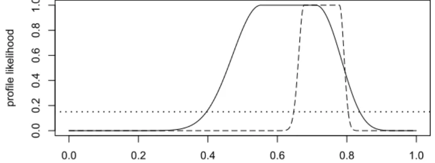
is defined by g(P)={PV{1}}for all P∈ P). The induced profile likelihood function likgon[0,1]is plotted in Figure 1
for the cases with(n0,n1,n01)=(11,21,6)and(n0,n1,n01)=(213,651,98): solid and dashed lines, respectively (a detailed calculation of likgis given in Example 4).
In these two cases, the likelihood-based confidence regions with cutoffpointβ=0.15for the probability PV{1}
are approximately the intervals[0.39,0.84]and[0.65,0.80], respectively (the cutoffpointβ=0.15is represented by the dotted line in Figure 1). They are (conservative) confidence intervals of approximate level95%(see for example [22]). 0.0 0.2 0.4 0.6 0.8 1.0 0.0 0.2 0.4 0.6 0.8 1.0 profile lik elihood
Figure 1: Profile likelihood functions from Examples 3 and 4.
2.3. Likelihood for Imprecise Data Models
In the situation we consider, we are actually interested in the (unobserved) precise data Vi. In this case, the
characteristic of interest (described byg) depends only on the marginal distributionPVof the precise dataVi; that is,
we can writeg(P)=:g′(PV) for allP∈ P. For example, thep-quantile of the distribution ofh(Vi) depends only on
the distribution ofVi. By contrast, as noted at the beginning of Subsection 2.2, the valuelik(P) depends only on the
marginal distributionPV∗of the imprecise dataVi∗. By writinglik(P)=lik∗(PV∗) for allP∈ P, we define a function
lik∗:PV∗→[0,1], which can be interpreted as the likelihood function onPV∗.
In order to obtain the profile likelihood functionlikg, it can be useful to consider the multivalued mappingg∗from
PV∗toGdefined by g∗(P V∗)= [ PV∈[PV∗] g′(P V)
for allPV∗ ∈ PV∗. The multivalued mappingg∗ assigns to eachPV∗ all the values that the characteristic described
byg′ takes on the set [PV∗] of all distributions for the precise dataVi compatible with the distributionPV∗ for the
imprecise dataV∗
i. That is,g∗can be interpreted as an imprecise version ofg′, assigning to each imprecise probability
distribution [PV∗] the corresponding imprecise value ofg′.
We can now define the functionlik∗
g∗:G →[0,1] in analogy with the expression for the profile likelihood function
likggiven in Lemma 1:
lik∗
g∗(γ)= sup
PV∗∈PV∗:γ∈g∗(PV∗)
lik∗(P
V∗)
for allγ∈ G(where the supremum is 0 when noPV∗satisfies the condition). The functionlik∗g∗can be interpreted as the
profile likelihood function induced by the multivalued mappingg∗, whenlik∗is considered as the likelihood function
onPV∗. This profile likelihood function is particularly interesting in connection with the discussion of Subsection 2.1,
becauselik∗describes the statistical uncertainty about the distributionPV∗of the imprecise dataV∗
i, which decreases
when we observe more and more (imprecise) data, whileg∗describes the (unavoidable) indetermination of the values
ofg (in the terminology of [24], the values ofg∗ are the identification regions for the values ofg). Thanks to the
following result, the profile likelihood functionlik∗
g∗ is not only interesting from a conceptual point of view, but also
useful in order to calculate the likelihood-based confidence regions for the values ofg. Lemma 2.
likg =lik∗g∗
Proof. From Lemma 1 and the above definitions it follows that for allγ∈ G, likg(γ)= sup P∈P:γ∈g′(PV)lik ∗(P V∗)= sup PV∗∈PV∗:∃P′∈P:PV′∗=PV∗∧γ∈g′(P′V) lik∗(P V∗)= sup PV∗∈PV∗:∃PV∈[PV∗] :γ∈g′(PV) lik∗(P V∗)=lik∗g∗(γ).
Example 4. The imprecise version g∗of the mapping g of Example 3 is the multivalued mapping fromPV∗to[0,1]
assigning to each PV∗ the set{PV{1}:PV ∈[PV∗]}. In Example 2 we have seen that, since nowε=0, this set is the
interval
[PV∗{1},PV∗{1}]=[PV∗{{1}},1−PV∗{{0}}].
That is, g∗(PV∗)is the interval probability that a precise data value Vi is1 (before observing the corresponding
imprecise data value V∗
i) according to the imprecise probability distribution[PV∗](i.e., the belief function onVwith
basic probability assignment PV∗).
As seen in Example 2, the only condition on the marginal distributions PV∗∈ PV∗is PV∗{∅}=0(since nowε=0).
That is,PV∗corresponds to the set of all probability distributions on the set{{0},{1},V}, and can thus be parametrized
by the2-dimensional simplex S2=
n
p=(p0,p1,p01)∈[0,1]3 :p0+p1+p01=1
o
.
Therefore, lik∗:PV∗→[0,1]corresponds to a (normalized) multinomial likelihood function, and we obtain
lik∗ g∗(γ)= max p∈S2:γ∈[p1,1−p0] pn0 0 pn11pn0101 ˆ pn0 0 pˆn11pˆn0101 for allγ∈[0,1], where
ˆ p= n0 n0+n1+n01, n1 n0+n1+n01, n01 n0+n1+n01 !
is the maximum likelihood estimate of the parameter p∈ S2. Hence, in particular, likg∗∗(γ)=1for allγ∈[ ˆp1,1−pˆ0]. Moreover, it can be easily proved that ifγ <pˆ1, then
p= p0ˆ 1−γ
1−p1ˆ , γ, p01ˆ 1−γ
1−p1ˆ
maximizes pn0
0 pn11pn0101among all p∈ S2such that p1≤γ. Symmetrically, if1−γ <p0, thenˆ p= 1−γ, pˆ11−γp0ˆ , pˆ01 1−γp0ˆ
!
maximizes pn0
0 pn11pn0101 among all p∈ S2such that p0≤1−γ. Altogether, thanks to Lemma 2, we obtain the following expression for the profile likelihood function induced by the multivalued mapping g (see also [38]):
likg(γ)=lik∗g∗(γ)= γ ˆ p1 !n1 1−γ 1−pˆ1 !n0+n01 if 0≤γ <pˆ1, 1 if pˆ1≤γ≤1−pˆ0, 1−γ ˆ p0 !n0 γ 1−p0ˆ !n1+n01 if 1−p0ˆ < γ≤1.
The profile likelihood function likg=likg∗∗on[0,1]is plotted in Figure 1 for the two cases considered in Example 3.
In the case with38data (solid line) there is (statistical) uncertainty also about the distribution PV∗of the imprecise
data V∗
i, while in the case with962 data (dashed line) almost only the (unavoidable) indetermination described by
g∗remains, in the sense that lik∗
g∗is almost equal to the indicator function of an identification region for PV{1}(more
precisely, the indicator function of the probability interval g∗( ˆPV∗) = [ ˆp1,1−p0]ˆ corresponding to the maximum
likelihood estimate of PV∗∈ PV∗).
3. Regression
We now apply the results of Section 2 to the problem of regression with imprecisely observed variables. Hence, we assume that the (unobservable) precise data are pairsVi =(Xi,Yi), whereX1, . . . ,Xnarenrandom objects taking
values in a setX, andY1, . . . ,Ynarenrandom variables, withV=X ×R. For someV∗⊆2X×Rand someε∈[0,1],
we consider the fully nonparametric assumptionP=Pε. This means that we do not assume anything about the joint
distribution ofXiandYi, while the only condition on the joint distribution of the (unobserved) precise dataViand their
imprecise observationsV∗
i is given by assumption (1). In the remainder of the paper, we focus on this setting.
We want to describe the relation betweenXi andYiby means of a function f ∈ F, whereF is a particular set
of (measurable) functions f :X → R. In order to assess the quality of the description by means of f, we define the (absolute) residuals
Rf,i:=|Yi−f(Xi)|.
Thenrandom variablesRf,1, . . . ,Rf,n ∈[0,+∞) are independent and identically distributed: the more their distribution
is concentrated near 0, the better is the description by means of f.
In order to compare the quality of the descriptions by means of different functions f ∈ F, we need to compare
the concentration near 0 of the distributions of the corresponding residualsRf,i. Usual choices of measures for this
concentration are the second and first momentsE(R2
f,i) andE(Rf,i), respectively. However, the moments of the
dis-tribution of the residuals cannot be really estimated in the fully nonparametric setting we consider, because moments are too sensitive to small variations in the distribution (see also Subsection 4.2). In fact, ifε >0 or the set
Rf :={|y−f(x)|: (x,y)∈A,A∈ V∗}
(i.e., the set of all possible values ofRf,iwhenVi∈Vi∗) is unbounded, then the likelihood-based confidence region for
any particular moment of the distribution of the residuals is unbounded (even when only the distributions with finite moments are considered), independently of the cutoffpoint and of the observed (imprecise) data.
By contrast, the quantiles of the distribution of the residuals can in general be estimated even in the fully nonpara-metric setting we consider. Therefore, we propose to use the p-quantile of the distribution of the residualsRf,i as a
measure of the concentration near 0 of this distribution, for somep∈(0,1). The technical details of the estimation of such quantiles are given in Subsections 3.1 and 3.2.
The minimizations of the second and first moments of the distribution of the residuals can be interpreted as the theoretical counterparts of the methods of least squares and least absolute deviations, respectively. In the same sense,
the minimization of thep-quantile of the distribution of the residuals can be interpreted as the theoretical counterpart of the method of least quantile of squares (or absolute deviations), introduced in [29] as a generalization of the method of least median of squares (corresponding to the choicep = 0.5). The method of least quantile of squares leads to robust regression estimators, with breakdown point min{p,1−p}(that is, the highest possible breakdown point 50% is reached when p=0.5). By contrast, the methods of least squares and least absolute deviations lead to regression estimators with breakdown point 0, since they cannot even handle a single outlier (including leverage points; see for example [18, 26, 21]).
In the location problem (that is, when F is the set of all constant functions f : X → R), the values of the constant functionsf minimizing the second and first moments of the distribution of the residualsRf,iare the mean and
median of the distribution ofYi, respectively (when these exist and are unique). The value of the constant function f
minimizing the p-quantile of the distribution of the residualsRf,iis the p-center of the distribution ofYi(that is, the
center of the shortest interval containingYiwith probability at leastp), when this exists and is unique. Thep-center
can be interpreted as a generalization of the mode of a distribution, since under some regularity conditions the mode corresponds to the limit of thep-center whenptends to 0. Thep-center of a symmetric, strictly unimodal distribution corresponds to its median and mean (when this exists), independently of p. Therefore, the minimizations of the p-quantile, first moment, and second moment of the distribution of the residuals lead to the same (correct) regression function, under the usual assumptions for the error distribution: see for example [33].
Example 5. We consider a problem of simple linear regression: that is,X=R(and thusV=R2), andF ={fa,b :
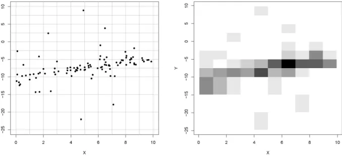
a,b∈R}is the set of all linear functions fa,bdefined by fa,b(x)=a+b x for all x∈R. The left plot of Figure 2 shows
n=99precise data points V1, . . . ,Vn. However, we assume that the pairs of precise values Vi=(Xi,Yi)∈R2are not
known. Instead, for given partitions of the real line in intervals, we only know in which intervals X∗
i and Yi∗lie Xiand
Yi, respectively. That is, we assume that only the imprecise data V1∗, . . . ,Vn∗are observed, where Vi∗ =Xi∗×Yi∗, and
the elements ofV∗ (i.e., the possible imprecise observations V∗
i) build a partition ofV =R2 (hence, in particular,
Rf = [0,+∞)). This partition is represented in the left plot of Figure 2 (gray lines), while the right plot is the
corresponding two-dimensional histogram of the data set.
Figure 2: Data set from Examples 5, 6, 7, 8, and 9: (unobserved) precise dataVi =(Xi,Yi)∈R2and partition ofR2(left), and corresponding
two-dimensional histogram representing the observed (imprecise) dataV∗
i =X∗i ×Yi∗⊂R2.
3.1. Determination of Profile Likelihood Functions for Quantiles of Residuals
We want to determine the likelihood-based confidence regions for the quantiles of the distribution of the residuals: for this purpose, we calculate the profile likelihood function for such quantiles. Letp ∈(0,1), and for each function
f ∈ F, letQf be the interval defined byQf =Lf∩ Uf, with
Lf =
[
r∈Rf [r,+∞)
whenp> εandLf =[0,+∞) otherwise, while
Uf =
[
r∈Rf [0,r]
whenp<1−εandUf =[0,+∞) otherwise. The definition ofQf can be interpreted as follows: ifε <p<1−ε, then
Qf is the smallest interval containingRf, while ifp ≤ε, then this interval is extended to the left until 0 (included),
and ifp≥1−ε, then it is extended to the right until+∞(not included). Therefore,Qf is the set of all possible values
for thep-quantile of the distribution of the residualsRf,i, sinceP(Rf,i<Rf)≤εfollows from assumption (1).
For each f ∈ F, letQf be the multivalued mapping fromPtoQf assigning to each probability measurePthe
p-quantile of the distribution of the residualsRf,iunderP. As noted in Subsection 2.2, the mappingQfis multivalued,
because in general quantiles are not uniquely defined. We want to determine the profile likelihood functionlikQf : Qf → [0,1] induced by the multivalued mapping Qf. It is important to note that we would obtain the same results
by considering only the distributions for which the p-quantile is unique (that is, the vagueness in the definition of quantiles has no influence on the resulting likelihood-based confidence regions).
Assume that the (imprecise) dataV∗
1 = A1, . . . ,Vn∗ = An are observed, whereA1, . . . ,An ∈ V∗\{∅}. In order to
obtain the profile likelihood functionlikQf for thep-quantile of the distribution of the residualsRf,i, we define for each
function f ∈ F and each distanceq∈[0,+∞) the bands
Bf,q:={(x,y)∈ V:|y−f(x)| ≤q},
Bf,q:={(x,y)∈ V:|y−f(x)|<q} and the functionskf,kf on [0,+∞) such that
kf(q)=# n i∈ {1, . . . ,n}:Ai∩Bf,q,∅ o , kf(q)=#ni∈ {1, . . . ,n}:Ai⊆Bf,qo
for allq ∈ [0,+∞) (where #Adenotes the cardinality of a set A). That is, kf(q) is the number of imprecise data
intersectingBf,q, whilekf(q) is the number of imprecise data completely contained inBf,q. Therefore, in particular,
kf andkf are monotonically increasing functions ofq, andkf(q)≤kf(q) for allq∈ [0,+∞). Finally, we define the
functionλ: [0,1]×(0,1)→(0,1] as follows, for alls∈[0,1] and allt∈(0,1):
λ(s,t)= 1−t if s=0, t s s 1−t 1−s !1−s if 0<s<1, t if s=1.
Theorem 1. For each f ∈ F, the profile likelihood function likQf for the p-quantile of the distribution of the residuals Rf,ican be expressed as follows, for all q∈ Qf:
likQf(q)= λ kf(q) n ,p−ε !n if kf(q)<(p−ε)n, 1 if hkf(q),kf(q) i ∩(p−ε)n,(p+ε)n,∅, λ kf(q) n ,p+ε !n if kf(q)>(p+ε)n. (2)
Proof. In order to prove expression (2), we use Lemma 2, which tells us that likQf(q) = lik∗Q∗
f(q) for all q ∈ Qf, wherelik∗andQ∗
f are defined on the setPV∗of all possible distributionsPV∗for the imprecise dataVi∗. The function
lik∗assigns to eachPV∗the corresponding likelihood value: in particular, it has a unique maximum in the empirical
distribution (of the imprecise data) ˆPV∗. The multivalued mappingQ∗f assigns to each PV∗ all p-quantiles of the
residualsRf,ifor all distributions of the precise dataVicompatible withPV∗.
We first consider the empirical distribution (of the imprecise data) ˆPV∗: we know that lik∗( ˆPV∗) = 1, and we
want to determineQ∗
f( ˆPV∗). Each joint distribution ofViandVi∗with marginal distribution ˆPV∗can be described by
the conditional distributions ofVi givenVi∗ = Aj (for each imprecise observationAj), since ˆPV∗{A1, . . . ,An} = 1.
In particular, for each q ∈ Qf we can construct a joint distribution ofVi andVi∗ as follows: for each one of the
kf(q)−kf(q) imprecise observationsAjsuch that (Bf,q\Bf,q)∩Aj,∅, we can choose the conditional distribution of
VigivenVi∗=Ajto be concentrated on (Bf,q\Bf,q)∩Aj, while for all other imprecise observationsAj, we can choose
the conditional distributions ofVigivenVi∗ =Ajin such a way that as little probability as possible is given toBf,q,
and as much as possible toBf,q\Bf,q, according to assumption (1). The resulting probability distribution satisfies
P(Rf,i<q)=PV(Bf,q)=max kf(q) n −ε,0 ! = min P′ V∈[ ˆPV∗]P ′ V(Bf,q), P(Rf,i≤q)=PV(Bf,q)=min kf(q) n +ε,1 ! = max P′ V∈[ ˆPV∗] P′ V(Bf,q), and therefore, q∈Q∗ f( ˆPV∗)⇔ kf(q) n −ε≤p≤ kf(q) n +ε⇔ h kf(q),kf(q) i ∩(p−ε)n,(p+ε)n,∅. This proves the second case of expression (2).
We now prove the first case of expression (2), and thus assume thatq∈ Qf satisfieskf(q)<(p−ε)n. Ifqis a
p-quantile according toP∈ P, thenP(Vi∈Bf,q)=P(Rf,i≤q)≥p, and assumption (1) impliesP(Vi∈Vi∗∩Bf,q)≥p−ε.
This is more than what the empirical distribution ˆPV∗ assigns to thekf(q) imprecise data intersectingBf,q, and it can
be easily proved that all marginal distributionsPV∗∈ PV∗maximizinglik∗among the ones satisfyingq∈Q∗f(PV∗) can
be expressed as
PV∗=(p−ε)P′V∗+(1−p+ε)P′′V∗, (3)
whereP′′
V∗ ∈ PV∗is the empirical distribution obtained when only then−kf(q) imprecise data not intersectingBf,qare
considered, and ifkf(q)>0, thenPV′∗ ∈ PV∗is the empirical distribution obtained when only thekf(q) imprecise data
intersectingBf,qare considered. In this case,PV∗is unique, while ifkf(q)=0, thenP′V∗∈ PV∗can be any distribution
assigning the whole probability to elements ofV∗intersectingBf
,q. Such elements ofV∗exist, becausep> ε(since
kf(q)<(p−ε)n), and therefore the definition ofQf implies that there is anr∈ Rf such thatr≤q. Ifkf(q)>0, then
for the unique marginal distributionPV∗of the form (3) we have
lik∗(P V∗)= Qn i=1PV∗{Ai} Qn i=1PˆV∗{Ai} = p−ε kf(q) kf(q) 1−p+ε n−kf(q) n−kf(q) 1 n n = pkf−(q)ε n kf(q) 11−−(pkf−(q)ε) n n−kf(q) =λ kf(q) n , p−ε !n , while ifkf(q)=0, then for all marginal distributionsPV∗of the form (3) we have
lik∗(P V∗)= Qn i=1PV∗{Ai} Qn i=1PˆV∗{Ai} = 1−p+ε n n 1 n n =(1−(p+ε))n=λ(0, p−ε)n.
These two expressions forlik∗(P
V∗) are valid also when some of the imprecise observationsA1, . . . ,An are equal,
because in this case additional factors appear in the numerator as well as in the denominator of the fractions expressing the likelihood ratio ofPV∗and ˆPV∗(see for instance also [27, Section 2.3]). This proves the first case of expression
The expression forlikQf given in Theorem 1 is very general, but rather involved. To obtain a simpler result about likQf, we define, for each function f ∈ F and each imprecise dataAi, the infimumrf,iand the supremumrf,iof the set
of all possible values of the residualRf,iwhenVi∈Ai(i.e., when the imprecise observationVi∗=Aiis correct):
rf,i= inf
(x,y)∈Ai|y−f(x)|, rf,i= sup
(x,y)∈Ai
|y−f(x)|.
As usual in statistics,rf,(i) andrf,(i) denote then theith smallest infimum and supremum, respectively, so that with rf,(0) := rf,(0) := infQf andrf,(n+1) := rf,(n+1) :=supQf we obtainrf,(0) ≤ . . . ≤ rf,(n+1)andrf,(0) ≤ . . . ≤rf,(n+1). Finally, we definei:=max (⌈(p−ε)n⌉,0) andi:=min (⌊(p+ε)n⌋,n)+1, so thati∈ {0, . . . ,n}andi∈ {1, . . . ,n+1},
withi≤i.
Lemma 3. The points of discontinuity of the restriction of kf toQf, including the endpoints ofQf, are (in ascending
order, with possible repetitions) rf,(0), . . . ,rf,(n+1), and for all other values of q∈ Qf we have kf(q)=i if rf,(i)<q< rf,(i+1)with i∈ {0, . . . ,n}.
The points of discontinuity of the restriction of kf toQf, including the endpoints ofQf, are (in ascending order,
with possible repetitions) rf,(0), . . . ,rf,(n+1), and for all other values of q∈ Qf we have kf(q)=i if rf,(i) <q<rf,(i+1)
with i∈ {0, . . . ,n}.
Proof. The points of discontinuity of the restrictions ofkf,kf toQf, possibly including the endpoints ofQf, are (for
all imprecise dataAi)
inf{q∈ Qf :Ai∩Bf,q,∅}=inf n q∈ Qf :∃(x,y)∈Ai:|y−f(x)| ≤q o =inf{|y−f(x)|: (x,y)∈Ai}=rf,i, sup{q∈ Qf :Ai*Bf,q}=sup n q∈ Qf :∃(x,y)∈Ai:|y−f(x)| ≥q o =sup{|y−f(x)|: (x,y)∈Ai}=rf,i,
respectively, because (x,y) ∈ Ai implies|y−f(x)| ∈ Rf ⊆ Qf. Hence, if rf,(i) < q < rf,(i+1) withi ∈ {0, . . . ,n}, then there are exactlyi imprecise data intersecting Bf,q (i.e.,kf(q) = i). Analogously, ifrf,(i) < q < rf,(i+1) with i∈ {0, . . . ,n}, then there are exactlyiimprecise data completely contained inBf,q(i.e.,kf(q)=i).
Corollary 1. For each f ∈ F, the profile likelihood function likQf for the p-quantile of the distribution of the residuals Rf,iis a piecewise constant function, which can take at most n+2different values.
The points of discontinuity of likQf, including the endpoints ofQf, are (in ascending order, with possible repeti-tions)
rf,(0), . . . ,rf,(i),rf,(i), . . . ,rf,(n+1),
and for all other values of q∈ Qf,
likQf(q)= λi n, p−ε n if rf,(i)<q<rf,(i+1) with i∈ {0, . . . ,i−1} (when i≥1), 1 if rf,(i)<q<rf,(i), λi n, p+ε n if rf,(i)<q<rf,(i+1) and i∈ {i, . . . ,n} (when i≤n). (4)
Proof. The functionlikQf can take at mostn+2 different values, because in the first case of expression (2) the possible values ofkf(q) are the integersksuch that 0≤k<(p−ε)n, while in the third case the possible values ofkf(q) are the
integersksuch that (p+ε)n<k≤n(hence, in these two cases taken together,likQf can take at mostn+1 different values).
Ifi≥1, then 0≤i−1<(p−ε)n, and ifi≤n, thenn≥i>(p+ε)n. Hence, expression (4) is well-defined, and
in order to prove the second part of the corollary, it suffices to show that it holds for allq∈ Qf. This is easily done,
since expression (4) is a direct consequence of Theorem 1 and Lemma 3. In the first case of expression (4), Lemma 3 implieskf(q) =i <(p−ε)n, in the third case it implieskf(q)=i > (p−ε)n, while in the second case it implies kf(q)≥i≥(p−ε)nandkf(q)≤i−1≤(p+ε)n.
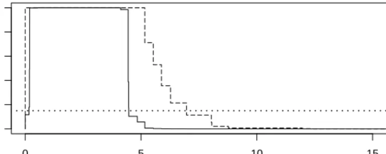
Example 6. In the problem of simple linear regression introduced in Example 5, let f ∈ F be the linear function plotted in Figure 4 (left, solid line). In this situation, the sets of all possible values of the residuals Rf,i(when the
imprecise observations V∗
i =Xi∗×Yi∗are correct) are intervals, and their endpoints rf,i,rf,ican be easily calculated.
They can then be used in expression (4), which determines the values of the profile likelihood function likQf for the p-quantile of the distribution of Rf,i(apart in its points of discontinuity, including the endpoints ofQf =Rf =[0,+∞)).
The function likQf with p=0.75is plotted in Figure 3 for the cases withε=0(solid line) andε=0.1(dashed line).
0 5 10 15 profile lik elihood 0.0 0.2 0.4 0.6 0.8 1.0
Figure 3: Profile likelihood functions from Examples 6 and 7.
3.2. Determination of Confidence Intervals for Quantiles of Residuals
Thanks to Theorem 1, we can now calculate, for each cutoffpointβ ∈ (0,1), the likelihood-based confidence regions for the quantiles of the distribution of the residualsRf,i. We obtain in particular the following result.
Corollary 2. Ifεis sufficiently small and n is sufficiently large so that
(max{p,1−p}+ε)n≤β (5) holds, then k:=max ( k∈ {0, . . . ,i−1}:λ k n, p−ε ! ≤pnβ ) , k:=min ( k∈ {i, . . . ,n}:λ k n, p+ε ! ≤pnβ )
are well-defined and satisfy
0≤k<(p−ε)n≤p n≤(p+ε)n<k≤n,
and for each f ∈ F, the likelihood-based confidence region with cutoffpointβfor the p-quantile of the distribution of the residuals Rf,iis the nonempty interval
Cf :=
n
q∈[0,+∞) :hkf(q),kf(q)
i
∩(k,k),∅o, whose lower and upper endpoints are rf,(k+1)and rf,(k), respectively.
Proof. Assumption (5) implies in particular (p−ε)n>0 andλ(0, p−ε)=1−p+ε≤√nβ, and thereforekis well-defined, sincei−1≥0 andk =0 satisfies the condition of the maximum. Analogously,kis well-defined, because
i≤nandk=nsatisfies the condition of the minimum, since (p+ε)n<nandλ(1, p+ε)=p+ε≤√nβfollow from assumption (5). The definitions ofkandkimply in particular the inequalities 0≤k<(p−ε)nand (p+ε)n<k≤n. We now prove that Cf is the likelihood-based confidence region with cutoff pointβfor the p-quantile of the
distribution of the residualsRf,i(that is, for the values of the multivalued mappingQf). From the definition of profile
likelihood function given in Subsection 2.2 it follows that this confidence region is the set of allq ∈ Qf such that
likQf(q)> β. We can thus use Theorem 1 to determine the confidence region. It can be easily proved that for each t ∈ (0,1) considered as a constant, λis a continuous function of s ∈ [0,1], monotonically increasing on [0,t] and
monotonically decreasing on [t,1]. Therefore, in the first case of expression (2) we havelikQf(q) > βif and only if kf(q)>k, while in the third case we havelikQf(q)> βif and only ifkf(q)<k. Altogether, we obtain thatlikQf(q)> β if and only ifhkf(q),kf(q)
i
∩(k,k),∅, since(p−ε)n,(p+ε)n⊂(k,k). It remains to show thatq∈ Cf implies
q∈ Qf. Ifq∈ Cf, thenkf(q)>0, and so there is anr∈ Rf such thatr≤q. Analogously, ifq∈ Cf, thenkf(q)<n,
and so there is anr∈ Rf such thatr≥q. Hence,q ∈ Cf impliesq∈ Qf, and thereforeCf is the desired confidence
region.
The setCf is an interval, since the functionskf,kf are monotonically increasing, andkf(q) ≤kf(q) for allq ∈
[0,+∞). Moreover, the definition of likelihood function implies that there is a probability measureP ∈ Psuch that
lik(P) > β, and therefore Cf is not empty, because Qf(P) ⊆ Cf follows from the definition of likelihood-based
confidence region. Finally, Lemma 3 implies
infCf =infnq∈[0,+∞) :kf(q)>ko=rf,(k+1), supCf =sup n q∈[0,+∞) :kf(q)<k o =rf,(k),
sincekf(q)=nfor allq∈[0,+∞)\ Uf, andkf(q)=0 for allq∈[0,+∞)\ Lf.
The intervalCf defined in Corollary 2 consists of allq∈[0,+∞) such that the bandBf,qintersects at leastk+1
imprecise data, and the bandBf,qcontains at mostk−1 imprecise data. Whenε=0, the intervalCf is asymptotically
a (conservative) confidence interval of levelFχ2(−2 logβ) for the p-quantile of the distribution of the residualsRf,i,
whereFχ2 is the cumulative distribution function of the chi-square distribution with 1 degree of freedom (see for
example [27]). The finite-sample level of the (conservative) confidence intervalCf can be obtained directly from its
definition, by means of simple combinatorial arguments (also whenε > 0), but this goes beyond the scope of the
present paper.
It is important to note that the confidence intervalsCf do not depend on the choice of the set V∗ of possible
imprecise data (as far as the observed ones, A1, . . . ,An, are contained in it). This can be surprising, since the set
P=Pεof probability measures considered depends strongly onV∗, as noted at the beginning of Section 2. However,
the independence of the confidence intervalsCf from the choice of the setV∗is not so surprising when one considers
that the intervalsCfare likelihood-based confidence regions, and that likelihood inference is always conditional on the
data (that is, independent of considerations about which other data could have been observed). This can be considered as a sort of robustness against misspecification of the setV∗of possible imprecise data. The practical advantage is
that it is not necessary to think about which other imprecise data could have been observed, besides the ones that were actually observed (that is,A1, . . . ,An).
Example 7. In the situation of Example 6, the confidence intervalCf withβ = 0.15is approximately[0.16,4.47]
whenε=0, and[0,6.96]whenε=0.1(the cutoffpointβ=0.15is represented by the dotted line in Figure 3).
3.3. Regression as a Decision Problem
The problem of minimizing the p-quantile of the distribution of the residualsRf,ican be described as a statistical
decision problem: the set of probability measures considered isP=Pε, the set of possible decisions isF, and the
loss functionL:P × F →[0,∞) is defined by
L(P,f)=Qf(P)
for allP ∈ Pand all f ∈ F. That is, thep-quantile of the distribution of the residualsRf,iis interpreted as the loss
we incur when we choose the function f. In fact, the loss functionLis multivalued, since in general thep-quantile is not unique: L(P,f) could be reduced to a single value by taking for example the upperp-quantile of the distribution of the residualsRf,i.
The information provided by the observed (imprecise) data is described by the likelihood functionlikonP. A very simple way of using this information consists in reducingPto the setP>βfor some cutoffpointβ∈(0,1). The
resulting setP>βcan be interpreted as an imprecise probability measure, on which we can base our choice of f. For
each f ∈ F, the set of all possible values of the lossL(P,f) whenPvaries inP>βcan be interpreted as the imprecise
p-quantile of the residualsRf,iunder the imprecise probability measureP>β. It corresponds to the intervalCf, when
Assume that condition (5) is satisfied. In order to choose a function f, we can minimize the supremum ofCf.
This approach is similar to theΓ-minimax decision criterion with respect to the imprecise probability measureP>β,
and is called LRM (Likelihood-based Region Minimax) criterion in [7]. When there is a unique f ∈ F minimizing supCf (i.e., minimizing rf,(k)), it can be denoted by fLRM, and supCf can be denoted by qLRM. In this case, fLRM
is characterized geometrically by the fact thatBfLRM,qLRM is the thinnest band of the form Bf,q containing at leastk
imprecise data, for all f ∈ F and allq∈[0,+∞). Therefore, in order to find the function fLRM, it suffices to adapt to
the case of imprecise data the algorithms for the method of least quantile of squares (see for example [29, 36, 3]), but this goes beyond the scope of the present paper.
An interesting description of the uncertainty about the optimal choice of f ∈ F is obtained by considering interval dominance for the imprecisep-quantiles of the residualsRf,iunder the imprecise probability measureP>β. WhenfLRM
exists, the undominated functions f ∈ F are those such thatCf intersectsCfLRM. In particular, whenqLRM ∈ CfLRM (that is,CfLRM is right-closed), the undominated functions f ∈ F are characterized geometrically by the fact that Bf,qLRM intersects at least k+1 imprecise data. In general, the set of undominated functions f can be interpreted as the imprecise result of the regression: it describes the complex uncertainty about the optimal choice of f ∈ F. When we observe more and more (imprecise) data, the statistical uncertainty diminishes, but the set of undominated functions does not necessarily tend to reduce to a singleton, because of the (unavoidable) indetermination discussed in Subsection 2.1 (see also [10] for a more detailed analysis).
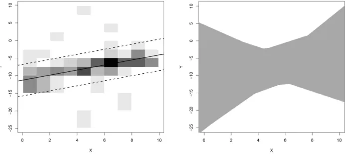
Example 8. Consider the problem of simple linear regression introduced in Example 5, withε = 0 (that is, the
classification of the precise data into the elements ofV∗ is assumed to be correct), p = 0.75, and β = 0.15. The
thinnest band of the form Bf,q (for all f ∈ F and all q ∈ [0,+∞)) containing at least k = 83imprecise data is
represented by the dashed lines in the left plot of Figure 4. It is the band BfLRM,qLRM, where fLRM is also plotted in Figure 4 (left, solid line), while qLRM =supCfLRM =rfLRM,(83) ≈4.47, as we have seen in Example 7. The right plot of Figure 4 shows the undominated functions f ∈ F (gray lines), which are characterized by the fact that the band Bf,4.47intersects at least k+1=67imprecise data.
Figure 4: FunctionfLRM(left, solid line), bandBfLRM,qLRM(left, dashed lines), and set of undominated functions (right, gray lines) from Example 8.
3.4. Prediction
Consider the case in which (instead ofn) we haven+1 pairs (Vi,V∗
i) of precise and imprecise dataVi=(Xi,Yi)
andV∗
i, respectively. We want to predict the realization of the precise data valueVn+1on the basis of the realization of thenimprecise dataV∗
1, . . . ,Vn∗. Choosek∈ {1, . . . ,n}, and assume that for each possible realization of then+1
imprecise dataV∗
is a thinnest band of the formBf,qcontaining at leastkof then+1 imprecise data, for all f ∈ F and allq∈[0,+∞).
Because of symmetry, the probability thatV∗
n+1is included in a bandBf,q′containing at leastkof then+1 imprecise
data (for some f ∈ F) is at leastk/(n+1). Hence, whenBf′′,q′′is a thinnest band of the formBf,qcontaining at leastkof
thenimprecise dataV∗
1, . . . ,Vn∗(for all f ∈ F and allq∈[0,+∞)), the probability thatVn∗+1is included in the union Bof all bandsBf,q′′ containing at leastk−1 of thenimprecise dataV1∗, . . . ,Vn∗(for all f ∈ F) is at leastk/(n+1). That
is,Bis a (conservative) prediction region of levelk/(n+1)−εfor the precise data valueVn+1.
In particular, when condition (5) is satisfied and fLRM exists, the unionBof all bandsBf,qLRM containing at least k−1 of then imprecise dataV∗
1, . . . ,Vn∗ (for all f ∈ F) is a (conservative) prediction region of levelk/(n+1)−εfor
the precise data valueVn+1. Prediction regions of this form can sometimes be reduced to smaller regions thanks to the assumption thatV∗
n+1takes values inV∗. When besides the realization of thenimprecise dataV1∗, . . . ,Vn∗, also the
(precise or imprecise) realization ofXn+1has been observed, the realization ofYn+1can be predicted for example by
using the idea of conformal prediction (see [35]), but this goes beyond the scope of the present paper.
Example 9. In the situation of Example 8, the unionBof all bands Bf,4.47containing at least82imprecise data (for all f ∈ F) corresponds to the region between the two curves in Figure 5. It is a (conservative) prediction region of levelk/(n+1)−ε=0.83for a future precise data point.
Figure 5: Prediction region from Example 9.
4. Example of Application
In this section, we apply the proposed regression method to socioeconomic data from the ALLBUS (German General Social Survey). Data collection in surveys is subject to many different influences that may cause various
biases in the data set (see for example [4]). Therefore, it is often reasonable to assume that the actual value lies rather in some interval around the observed value. Furthermore, data on sensitive quantities is sometimes only available in categories that form a partition of the space of possible values. A simple, ad hoc approach to analyze this kind of data is to reduce the intervals to their central values and to apply usual regression methods to the reduced, precise data. However, such an approach in general produces biased results (see [31, 2, 12]). In contrast to this, we suggest to analyze directly the interval-valued data by means of the regression method proposed in Section 3.
Here, we investigate how personal income varies with age, which is a fundamental relationship in the social sciences and a typical example in textbooks on social research methods (see for example [1]). Income is a key de-mographic variable in socioeconomic research questions, but asking for income in an interview is a sensitive question that some respondents refuse to answer. Therefore, survey data on personal income often include missing values. One
way to make the question less sensitive and thus to obtain better response rates is to present predefined income cate-gories (forming a partition of the range of possible income values) to the respondent according to which the personal income shall be classified. In the ALLBUS study, income data is collected by means of a two-step design with the open question for income as first step and the presentation of a category scheme as second step. As a result, the data set contains at the same time precise values for some individuals and interval-valued observations for others. Yet, even if the respondents answer the open question, they usually give only a rough estimate of their exact income, like a rounded or a heaped income value (see [19]), where heaping refers to irregular rounding behavior (see for example [20]). Therefore, it is more reliable to regard also the precise income values as intervals, e.g. in considering as actual observations the income classes in which the precise values lie.
Data on the age of the respondents are more easily obtained, but these data are usually of limited precision. Often, the age is measured on a discrete scale, i.e.age∈N. In that case, the information contained in a data value is that the actual age of the respondent lies in the interval [age,age+1). Furthermore, also age data are sometimes provided as
a categorical variable taking values in a set of disjoint age classes forming a partition of the observation space of the continuous variableage.
4.1. ALLBUS Data and Regression Model
We analyze the ALLBUS data set of 2008 containing 3 469 interviews. The considered variables arepersonal income(on average per month in euros) andage. For our analysis we use the categorized income variablev389 with 22 possible income classes and the discrete age variablev154. (Detailed information about the data set can be found in [34].) Although the data set contains 1 063 precise income values and our regression method could also be applied to a data set with some precise and some imprecise observations (see [10]), we prefer to use the categorized income variable for the reasons mentioned above. Moreover, the age data are interpreted as intervals of length 1. Thus, for each individuali∈ {1, . . . ,3 469}we consider observationsV∗
i =X∗i ×Yi∗, whereX∗i =[agei,agei+1) is the interval
covering the age of respondentiandY∗
i =[yi,yi) is the interval of the corresponding income category. In the given
data set, there are 682 missing income values and 12 missing age values. Missing values are replaced by the entire observation space of each variable, i.e.X∗
i =X:=[18,100) orYi∗=Y:=[0,+∞), respectively. A two-dimensional
histogram of the data set is given in Figure 7 (left).
The relationship betweenageandincomeis usually modeled by a quadratic function inage(see for example [1]). Thus, the set of regression functions we consider here isF = {fa,b1,b2 : a,b1,b2 ∈ R},where each function fa,b1,b2
is defined by fa,b1,b2(x) =a+b1x+b2x2 for all x ∈ X. We choose to minimize the median of the distribution of
the absolute residuals (i.e., p = 0.5), which is the choice of p implying the most robust results (see the beginning
of Section 3). As regards the cutoffpoint of the likelihood, we use a very high value: β = 0.9999. This choice
ofβcorresponds to the special case of LIR where we consider maximum likelihood (ML) estimates to evaluate the
regression functions fa,b1,b2 ∈ F (i.e.,k=i−1 andk=i). Note that in the present analysis the ML estimatesCfa,b1,b2
of the median of the absolute residuals are intervals, since the analyzed data set consists of proper sets (implying rf,i < rf,ifor each imprecise observationAi =X∗i ×Yi∗). Choosing the ML intervals means to ignore the statistical
uncertainty of the regression problem. A lower cutoffpointβwould imply a higher confidence level of the intervals Cfa,b1,b2 and lead to a more imprecise result. In the present analysis, the resulting set of undominated functions would
change only a little, because there is not much statistical uncertainty given the relatively large number of observations. Finally, as we consider only the income classes, we assume that the imprecise observations are correct and setε=0.
The effect of different choices ofβandεon the result of a LIR analysis has been studied thoroughly in [10].
For the present regression problem, we have implemented the LIR analysis as a grid search over the parameter spaceR3: First, the likelihood-based confidence regionsCfa,b1,b2 are computed for all regression functions correspond-ing to the parameter values (a,b1,b2) on a predefined grid. Then, we identify the parameter combination among these that minimizes the upper bound ofCfa,b1,b2. The function corresponding to this parameter combination is the function
fLRM which is optimal according to the LRM criterion (see Subsection 3.3). Finally, the upper boundqLRMofCfLRM is used to determine the set of undominated regression functions.
4.2. Results
We considered a grid of combinations of parameter values where a ∈ [−10 000,12 000], b1 ∈ [−200,250], andb2 ∈ [−10,10]. Corresponding to the set of undominated functions, we find the set of undominated parameter
combinations displayed in Figure 6. This set is clearly not convex. Moreover, in the case considered here, the parameters are not independent from each other, in the sense that many different combinations of parameter values
(a,b1,b2) may lead to very similar shapes of fa,b1,b2 overX. Thus, there are actually infinitely many undominated
parameter combinations, but the associated curves are similar to those we find within the considered grid.
Figure 6: Two-dimensional projections of the set of undominated parameter values.
The parameter combination implying the smallest upper endpoint of the ML interval for the 0.5-quantile of the residuals is (600,5,0) withCf600,5,0≈[270,680]. Thus, the function fLRMis a slightly increasing line. One
interpreta-tion of this funcinterpreta-tion is given by the bandBfLRM,qLRMlimited by the functions fLRM−qLRMand fLRM+qLRM: Among all bands (of any width) constructed around all considered functions,BfLRM,qLRM is the thinnest one that contains at least k=1 735 imprecise observations.
The function fLRM and the bandBfLRM,qLRM are presented in Figure 7 (right, black lines), besides the undominated functions (right, gray curves). As we considered ML estimates, no statistical uncertainty is reflected in the regression’s result, thus, the extent of the set of undominated functions is only due to the imprecision of the data. It can be seen that among the undominated functions there is a large variety of shapes of theage-incomeprofile, including straight lines, convex parabolic curves as well as concave ones. From a social scientist’s point of view this result may be unsatisfying because it does not support only one form of the relationship betweenageandincome. However, it is reasonable to consider all shapes consistent with the imprecise data as possibleage-incomeprofiles. If the observed intervals were overlapping or if they constituted a finer partition of the space of possible observations, the set of undominated functions would be smaller. The effect of different degrees of imprecision of the data on the regression’s
result was studied in [10], where different versions of the ALLBUS data set were analyzed and their results compared.
In the present analysis, the set of undominated functions can be interpreted as the set of all plausible descriptions of theage-incomeprofile that reflects at the same time the indetermination induced by the imprecise data.
The common, simple method to analyze this kind of interval data is to conduct a quadratic least squares (LS) regression based on the interval centers ignoring the indetermination induced by the imprecision of the data. In this case, an upper limit for the highest income class [7 500,+∞) has to be set in order to compute the interval centers. Of
course, the choice of this upper limit has an impact on the estimates of the LS regression. The effect of two different
choices of the upper income limit is illustrated in Figure 8 (black dashed curves). The LS curves displayed there are based on interval centers with upper income limits 10 000 and 50 000, respectively. In contrast to the LS regression based on the interval midpoints, the regression method proposed in this paper can also be applied to unbounded data. Since in the LIR method the evaluation of the regression functions is based on quantiles of the distribution of the absolute residuals, the result is not sensitive to the extremes. If there were less thankbounded data, e.g. if there were more than 50% missing observations in the present data set, the result would be the entire setF of considered regression functions.
An improvement of the approach of an LS regression based on the interval centers could be achieved by consid-ering a robust variant of this approach, in which least median of squares (LMS) estimation is used. In this case, an upper income limit has to be fixed, but the estimated regression function is insensitive to the choice of the extreme values, since the regression is based on the median of the absolute residuals. The LMS curve estimated on the basis of
Figure 7: Two-dimensional histogram of the analyzed data set (left) and set of undominated functions (right, gray curves), minimax functionfLRM
(right, black solid line) and bandBfLRM,qLRM(right, black dashed lines).
Figure 8: Set of undominated functions (gray curves) andfLRM(black solid line) of the LIR analysis versus LS curves based on interval centers
with upper limits 10 000 (lower black dashed curve) and 50 000 (upper black dashed curve), respectively, and LMS curve (black dotted line) based on interval centers with upper limit 50 000.
the interval centers with upper income limit 50 000 (black dotted line) and the function fLRMobtained from the LIR
analysis (black solid line) are also shown in Figure 8. These lines are similar to each other, which is not surprising as the proposed regression method can be seen as a generalization of the LMS regression to the case of imprecise data.
The proposed LIR method permits to identify plausible descriptions of the relationship between the socioeco-nomic characteristicsageandincome. Given the imprecise data, many different shapes of the age-income profile are
plausible. Further computations indicated that our findings hold for transformed income data on the logarithmic scale, too. The results are not very informative, but reflect the indetermination induced by the imprecision of the data. One idea to obtain more informative results from categorized data could be to use many different category schemes during
the income data collection and thereby obtain a data set with overlapping categories. 5. Conclusion
In this paper, we introduced a new regression method for imprecise data, in which the error distribution is not constrained to a particular parametric family. The regression method is very robust and can be adapted to a wide range of practical settings, since it can be applied to all kinds of imprecise data, covering e.g. interval data, precise data, and missing data. In our method, the imprecise data are interpreted as the result of a coarsening process which can be informative, and even wrong with a certain probability.
The proposed method is derived from a general approach to regression with imprecise data, which we call Likelihood-based Imprecise Regression. It consists in identifying by means of likelihood inference all sufficiently
plausible regression curves, which are considered as the imprecise result of the regression analysis. The extent of the imprecise result reflects both kinds of uncertainty involved in a regression problem with imprecise data: statistical uncertainty and indetermination.
In future work, we intend to improve the implementation of our regression method, and to study its statistical properties in more detail. Moreover, we plan to investigate the consequences of stronger assumptions about the error distribution and the coarsening process, and the possibility of replacing in the decision problem the quantiles of the residuals by other loss functions.
References
[1] P.D. Allison, Multiple Regression, Pine Forge Press, 1998.
[2] A.E. Beaton, D.B. Rubin, J.L. Barone, The acceptability of regression solutions: Another look at computational accuracy, J. Am. Stat. Assoc. 71 (1976) 158–168.
[3] T. Bernholt, Computing the least median of squares estimator in timeO(nd), in: O. Gervasi, M.L. Gavrilova, V. Kumar, A. Lagan`a, H.P. Lee,
Y. Mun, D. Taniar, C.J.K. Tan (Eds.), Computational Science and Its Applications — ICCSA 2005, Springer, 2005, pp. 697–706. [4] P.P. Biemer, L.E. Lyberg, Introduction to Survey Quality, Wiley, 2003.
[5] L. Billard, E. Diday, Regression analysis for interval-valued data, in: H.A.L. Kiers, J.P. Rasson, P.J.F. Groenen, M. Schader (Eds.), Data Analysis, Classification, and Related Methods, Springer, 2000, pp. 369–374.
[6] A. Blanco-Fern´andez, N. Corral, G. Gonz´alez-Rodr´ıguez, Estimation of a flexible simple linear model for interval data based on set arithmetic, Comput. Stat. Data Anal. 55 (2011) 2568–2578.
[7] M. Cattaneo, Statistical Decisions Based Directly on the Likelihood Function, Ph.D. thesis, ETH Zurich, 2007.
[8] M. Cattaneo, Fuzzy probabilities based on the likelihood function, in: D. Dubois, M.A. Lubiano, H. Prade, M.A. Gil, P. Grzegorzewski, O. Hryniewicz (Eds.), Soft Methods for Handling Variability and Imprecision, Springer, 2008, pp. 43–50.
[9] M. Cattaneo, A. Wiencierz, Regression with imprecise data: A robust approach, in: F. Coolen, G. de Cooman, T. Fetz, M. Oberguggenberger (Eds.), ISIPTA ’11, Proceedings of the Seventh International Symposium on Imprecise Probability: Theories and Applications, SIPTA, 2011, pp. 119–128.
[10] M. Cattaneo, A. Wiencierz, Robust regression with imprecise data, Technical Report 114, Department of Statistics, LMU Munich, 2011.
[11] G. de Cooman, M. Zaffalon, Updating beliefs with incomplete observations, Artif. Intell. 159 (2004) 75–125.
[12] A.P. Dempster, D.B. Rubin, Rounding error in regression: The appropriateness of Sheppard’s corrections, J. R. Stat. Soc., Ser. B 45 (1983) 51–59.
[13] P. Diamond, Least squares fitting of compact set-valued data, J. Math. Anal. Appl. 147 (1990) 351–362.
[14] M.A.O. Domingues, R.M.C.R. de Souza, F.J.A. Cysneiros, A robust method for linear regression of symbolic interval data, Pattern Recognit. Lett. 31 (2010) 1991–1996.
[15] M.B. Ferraro, R. Coppi, G. Gonz´alez-Rodr´ıguez, A. Colubi, A linear regression model for imprecise response, Int. J. Approx. Reasoning 51 (2010) 759–770.
[16] S. Ferson, V. Kreinovich, J. Hajagos, W. Oberkampf, L. Ginzburg, Experimental Uncertainty Estimation and Statistics for Data Having Interval Uncertainty, Technical Report SAND2007-0939, Sandia National Laboratories, 2007.
[18] F.R. Hampel, E.M. Ronchetti, P.J. Rousseeuw, W.A. Stahel, Robust Statistics: The Approach Based on Influence Functions, Wiley, 1986. [19] J.U. Hanisch, Rounded responses to income questions, Allg. Stat. Arch. 89 (2005) 39–48.
[20] D.F. Heitjan, D.B. Rubin, Ignorability and coarse data, Ann. Stat. 19 (1991) 2244–2253. [21] P.J. Huber, E.M. Ronchetti, Robust Statistics, Wiley, 2nd edition, 2009.
[22] D.J. Hudson, Interval estimation from the likelihood function, J. R. Stat. Soc., Ser. B 33 (1971) 256–262.
[23] E.A. Lima Neto, F.A.T. de Carvalho, Centre and range method for fitting a linear regression model to symbolic interval data, Comput. Stat. Data Anal. 52 (2008) 1500–1515.
[24] C.F. Manski, Partial Identification of Probability Distributions, Springer, 2003.
[25] M. Marino, F. Palumbo, Interval arithmetic for the evaluation of imprecise data effects in least squares linear regression, Ital. J. Appl. Stat. 14 (2002) 277–291.
[26] R.A. Maronna, D.R. Martin, V.J. Yohai, Robust Statistics: Theory and Methods, Wiley, 2006.
[27] A.B. Owen, Empirical Likelihood, Chapman & Hall/CRC, 2001.
[28] Y. Pawitan, In All Likelihood, Oxford University Press, 2001.
[29] P.J. Rousseeuw, A.M. Leroy, Robust Regression and Outlier Detection, Wiley, 1987. [30] G. Shafer, A Mathematical Theory of Evidence, Princeton University Press, 1976.
[31] W.F. Sheppard, On the calculation of the most probable values of frequency-constants for data arranged according to equidistant divisions of a scale, Lond. M. S. Proc. 29 (1898) 353–380.
[32] V. Strassen, Meßfehler und information, Z. Wahrscheinlichkeitstheorie 2 (1964) 273–305.
[33] D. Tasche, Unbiasedness in least quantile regression, in: R. Dutter, P. Filzmoser, U. Gather, P.J. Rousseeuw (Eds.), Developments in Robust Statistics, Physica-Verlag, 2003, pp. 377–386.
[34] M. Terwey, S. Baltzer, ALLBUS Datenhandbuch 2008, GESIS, 2009.
[35] V. Vovk, A. Gammerman, G. Shafer, Algorithmic Learning in a Random World, Springer, 2005.
[36] G.A. Watson, On computing the least quantile of squares estimate, SIAM J. Sci. Comput. 19 (1998) 1125–1138.
[37] M. Zaffalon, E. Miranda, Conservative inference rule for uncertain reasoning under incompleteness, J. Artif. Intell. Res. (JAIR) 34 (2009)
757–821.