Visual Pattern Recognition using Unsupervised
Spike Timing Dependent Plasticity Learning
Daqi Liu
School of Computer Science University of Lincoln Brayford Pool, Lincoln, LN6 7TS
Email: [email protected]
Shigang Yue
School of Computer ScienceUniversity of Lincoln Brayford Pool, Lincoln, LN6 7TS
Email: [email protected]
Abstract—Neuroscience study shows mammalian brain only use millisecond scale time window to process complicated real-life recognition scenarios. However, such speed cannot be achieved by traditional rate-based spiking neural network (SNN). Compared with spiking rate, the specific spiking timing (also called spiking pattern) may convey much more information. In this paper, by using modified rank order coding scheme, the generated absolute analog features have been encoded into the first spike wave with specific spatiotemporal structural information. An intuitive yet powerful feed-forward spiking neural network framework has been proposed, along with its own unsupervised spike-timing-dependent plasticity (STDP) learning rule with dynamic post-synaptic potential threshold. Compared with other state-of-art spiking algorithms, the proposed method uses biologically plausible STDP learning method to learn the selectivity while the dynamic post-synaptic potential threshold guarantees no training sample will be ignored during the learning procedure. Furthermore, unlike the complicated frameworks used in those state-of-art spiking algorithms, the proposed intuitive spiking neural network is not time-consuming and quite capable of on-line learning. A satisfactory experimental result has been achieved on classic MNIST handwritten character database.
I. INTRODUCTION
Neuroscientists report human brain can only use a few tens of milliseconds to recognize the object in a very complicated real-life scenarios [1]. It is still an open question that how our brain can processes such huge amount of information in such short time window. With the development of the neuroscience, more and more attentions have been focused on the spiking neural network as it may be the fundamental processing mechanism of the mammalian brain.
Spiking neural network (SNN),the third generation of neural network [2] model, incorporates the temporal information into the processing procedure. Compared with the spiking rate, the exact spiking timings of spike trains, also called spiking pattern, convey the significant spatiotemporal information, which distinguish itself from other input spike trains. Unlike the rate-based SNN [3], [4], [5], [6], it is still possible for timing-based SNN to distinguish different classes even in short time window. Furthermore, Spike-timing-dependent plasticity (STDP) [7], [8], [9], [10], [11], a biological process that adjusts the efficacy of synaptic connections based on the relative timing of post-synaptic spike and its input pre-synaptic spike, has often been used to learn the selectivity of the input
image. One can use single neuron equipped with STDP to extract the repeating spiking pattern even its spike density is same as distractors [12]. STDP is an unsupervised learning rule, that means no prior information or teaching signal are needed for the learning procedure. It will adaptively change the synaptic efficacy and try to extract the most notable spiking pattern.
In order to survive in the ever-changing cruelty environment, visual pattern recognition is a basic living skill for human beings and animals. Interestingly, in most cases, they can successfully recognize the pattern within very short period after learning. Traditionally, classic image processing methods have been used to deal with this task. Even it may be the fundamental mechanism of our brain, the researches using bio-inspired spiking neural network are still quite immature.
In paper [13], the authors proposed a novel spiking neural network with supervised learning rule and temporal coding scheme to generate the spike pattern. Such SNN system and its supervised learning rule achieved relatively high correct classification rate when cross-validate the MNIST database. However, such supervised learning rule used in their paper needs prior information or teaching signals before really training the database and such prior information can be hard to obtain in some cases. Inspired by the paper [14], paper [15] uses the spiking neural network to simulate almost the same HMAX structure proposed in paper [14], and then uses radial basis function (RBF) to classify different classes. Specifically, the authors use STDP learning method to train a S1-C1-S2 pathway so that the intermediate S2 features can be obtained. Even the STDP learning procedure has been simplified and the authors assume the whole spike wave locates in a very short time window (thus uses an infinite time window), such method is still too complicated and time-consuming for most visual pattern recognition applications.
In this paper, a novel spike timing-based feed-forward spiking neural network has been proposed, along with its own unsupervised STDP learning rule and dynamic post-synaptic potential threshold. Compared with other state-of-art spiking algorithms, the proposed method uses biologically plausible STDP learning method to learn the selectivity while the dynamic post-synaptic potential threshold guarantees no training sample will be ignored during the learning procedure.
Furthermore, unlike the complicated frameworks used in those state-of-art spiking algorithms, the proposed intuitive spiking neural network is not time-consuming and quite capable of on-line learning. The layout of this paper can be summa-rized as follows: Section 2 introduces the framework of the proposed feed-forward spiking neural network, along with its neuron model and STDP learning rule. Section 3 depicts the experimental results, along with the analysis about the results. Finally, Section 4 summarizes this paper, discussing the advantages and limitations of the proposed method.
II. FRAMEWORK OF THE PROPOSED FEED-FORWARD SPIKING NEURAL NETWORK
The whole framework of the proposed feed-forward spiking neural network will be explained in this section. In real world, the visual pattern recognition scenario often contains vast data dimensions and exists significant variability in terms of inter-class and intra-inter-class. Thus, the first step in almost all visual pattern recognition tasks is to reduce data dimensionality, which means more generalized features need to be generated firstly. The final generated features should contain the most distinguishable and unchangeable characteristics of the origi-nal input image [16], [17]. Until now, the input data are still analog values, which need to be transferred to spike trains for further learning. Thus, a suitable spiking neural coding scheme will be used to encode the analog values to spiking trains.
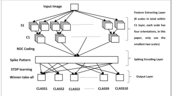
The proposed feed-forward spiking neural network can be summarized as following layers: feature extracting layer, spiking encoding layer and output layer. Fig.1 shows the framework of the proposed spike timing-based feed-forward spiking neural network. The whole procedure can be sum-marized as follows: Firstly, feature extracting layer computes C1 features with different scales and directions from input image. Then, Rank Order Coding transfers those C1 features into spike trains within the spiking encoding layer. Each input image has its own corresponding spike pattern after those two layers. Lastly, in the output layer, STDP learning rule and winner-take-all strategy have been used to train the synaptic efficacy matrix with specific selectivity to the input image. Notably, there is only one neuron (corresponding to specific class) within each output map in this paper. Below is the details of those three layers used in the proposed spiking neural network.
A. Feature Extracting Layer
It has been shown that visual processing is hierarchical, aiming to build an invariance to position and scale first and then to viewpoint and other transformations [18]. HMAX model [14], [19] uses a hierarchical system that closely follows the organization of visual cortex and thus built an increasingly complex and invariant feature representation by alternating between a template matching and a maximum pooling op-eration. Inspired by this computational model, Gabor filters with vary scales and orientations have been used to mimic the simple cells in the primary visual cortex and a further
Fig. 1: The framework of the proposed timing-based feed-forward spiking neural network.
Fig. 2: Gabor filter kernels with different scales and orienta-tions.
maximum pooling operation has been applied to generate the local invariance features.
Gabor response (F(σ,θx,y)) can provide a good model of cortical simple cell receptive fields (Fig.2 shows Gabor filter kernels with different scales and orientations), which can be described as follows: F(σ,θx,y)= exp − x 2 0+γ2y20 2σ2 ! ×cos 2π λx0 , s.t. (1)
x0=xcosθ+ysinθ; y0=−xsinθ+ycosθ (2) where x and y describes abscissa and ordinate of the input image, respectively.x0andy0represents abscissa and ordinate after rotating θ, respectively. γ represents aspect ratio, θ
depicts the orientation, σ is the effective width and λ the wavelength. In this paper, we choose the same parameters settings as the HMAX model that is using a range of sizes from7×7pixels to 37×37form the pyramid of scales, and four orientations(0o,45o,90o,135o)have been used. Notably,
the outputs have been normalized to a predefined range[−1,1]
so that input images with the same contrast will generate same features.
The local invariance features pool over retinotopically orga-nized afferent features from the previous layer with the same
orientation and from the same scale band, which simulate the complex cells existed within the primary visual cortex. There-fore, such local invariance features are tolerant to certain local transformations. Furthermore, the maximum pooling operation used to generate such local invariance features will greatly reduce the data dimensionality of the input image. Basically, the response rσ,θ(x,y) of a complex C1 unit corresponds to the maximum response of itsmafferentsF(σ,θx
1,y1),· · ·F σ,θ (xm,ym)
from the previous S1 layer with two adjacent scales:
rσ,θ(x,y)= max
j=1···mF σ,θ
(xj,yj) (3)
In visual cortex, cortical complex cells tend to have larger receptive fields compared with simple cells. In this paper, only the first two smallest scales have been used to generate the local invariance features. The whole procedure can be summarized as follows: Firstly, the Gabor filters with adja-cent scales and four different orientations have been used to mimic the simple cells within the primary visual cortex. The parameter settings for the Gabor filters are almost same as HMAX model. Secondly, for each orientation of the Gabor filter output with the smallest scale, a local sliding window with the size of 8×8 has been applied to generate the local invariance feature (Notably, there are overlaps between two adjacent sliding windows and the overlapping size is4×4). For the second smallest scale, the sliding windows size is10×10
and the overlapping size is 5×5.
In a word, the feature extracting layer used in this paper mimic the cortical simple cells with Gabor filter units and complex cells by maximum pooling operations. Template matching operation generates orientation edge packages with certain selectivity, while maximum pooling operation achieves dimensionality reduction and invariance to local transforma-tion.
B. Spiking Encoding Layer
Both spiking rate and spiking timing can be used to rep-resent the structural information of the input image. Tradi-tionally, researchers use spiking rate as the representation of the structural information within the input visual stimuli. However, recent neuroscience studies show that mammalian brain only use millisecond scale time window to process the complicated real-life visual recognition tasks, which means there is not enough time for rate-based SNN to generate meaningful spiking rates. Moreover, if the spiking rate of the background neural noise is same as the input visual stimuli, it is almost impossible for rate-based SNN to evolve the selectivity [12].
Luckily, with the developments of neuroscience, researchers found the specific spiking timing of each fired neuron itself conveys much more important structural information than the spiking rate. By gathering the spiking timings of the fired neurons together, we can obtain the spiking pattern with significant spatiotemporal structural information. Even the spiking rate remains the same, it is still possible to generate countless spiking patterns and each of them corresponds to
Fig. 3: Rank order coding scheme diagram.
a different input visual stimuli. Therefore, compared with rate-based SNN, timing-based SNN is more powerful and biologically plausible.
1) spiking encoding scheme: Rank order coding scheme [20], [21], [22], a time-to-first-spike coding scheme (one kind of temporal coding scheme), has been used to generate spike trains from the features extracted in the previous layer. Fig.3 shows the rank order coding scheme diagram. It can be seen that this kind of scheme only generate one spike after the corresponding unit receiving the input. The delay of the spiking timing is a monotonically decreasing function of the input analog value. Thus, the maximum analog input value corresponds to the minimum spiking timing delay. Pixels with less Input analog values will not generate spikes at all since their spiking timings have already exceeded a predefined time-window for spiking encoding layer (50 ms
for this paper). Through such coding scheme, only those units with more significant C1 features will be generating spikes. Notably, only one spike will be generated for each unit in rank order coding scheme. Such coding scheme is intuitive yet powerful. Given the reference timestamp (the beginning time of the encoding procedure), it transforms each analog value into corresponding relative spike time associated with the reference timestamp. Either the onset of external stimuli or the background oscillation can be considered as the reference timestamp. Although sometimes it is hard to find these kinds of reference timestamps during the real world learning procedure, it is intuitive to use the onset of C1 features as the reference timestamp in the proposed spiking neural network. Another drawback of the classical rank order coding scheme is that its distinguishability (or selectivity) remains at a relatively low level if using the traditional relative coding method [21].
In this paper, we linearly modified the original rank order coding scheme so that absolute spiking timing instead of relative spiking timing [21] has been generated. For one specific feature response (depicted asr) within C1 layer, the corresponding spiking timing (s) can be computed as follows:
s=p∗(max(r)−r) (4) wheremax (r)is the maximum value of all related C1 features in the receptive filed and pis a positive constant within the range from 0 to 1 (ptakes 0.25 in this paper).
2) neural model: Leaky integrate-and-fire neuron model acts as a coincidence detector and the causality between local spikes has been emphasized. When the post-synaptic neuron receives a spike from its pre-synaptic neuron, the responding
post-synaptic potential (PSP) will be generated. One can use certain time course to depict this dynamic PSP change. In leaky integrate-and-fire model, the post-synaptic potential will gradually decrease if no spikes received since last received spike. Therefore, in order to generate a post-synaptic spike, this post-synaptic neuron needs to receive lots of spikes within a relative small time window so that its PSP can reach the predefined threshold. The dynamic procedure of leaky integrate-and-fire model can be summarized as follows: when a post-synaptic neuron receives pre-synaptic spikes, it will generate dynamic synaptic current and this dynamic current will thus produce dynamic synaptic voltage. A post-synaptic spike will fired if the dynamic synaptic voltage reaches the predefined post- synaptic potential threshold. The dynamic post-synaptic current can be expressed as follows:
Ii(t) = X j wij X f αt−t(jf) (5) where t(jf) represents the time of the f-th spike of the j -th pre-synaptic neuron; wij is the strength of the synaptic
efficacy between neuroniand neuronj.α(t)is the time course function, which can be expressed as follows:
α(t) =α1 τexp −t τ Θ (t) (6)
where Θ is the Heaviside step function with Θ (t) = 1 for
t >0 andΘ (t) = 0 else.τ is the time constant. For a given time-varying input currentI (t), the dynamic voltageV (t)can be computed as follows: V(t) =Vrexp −t−t0 τm + R τm Z t−t0 0 exp − s τm I(t−s)ds (7)
where the initial condition V (t0) = Vr and τm is the
membrane time constant. R represents the resistance. This equation describes the dynamics of the membrane potential between successive spiking events. When the membrane po-tential reaches the threshold, it will fire a spike, followed by the absolute refractory period (resets to Vr) and then start to
evolve afterwards.
In this paper, a dynamic post-synaptic potential threshold has been proposed in the training period. For each input image, we do not set post-synaptic potential threshold for the first run and collect the generated dynamic voltage due to the input spike pattern. And then the maximum value of the dynamic voltage needs to be found after collecting all dynamic voltage within the predefined time window. Finally, the associated post-synaptic potential threshold has been set to a percentage of this maximum value. By doing this, each input image can be ensured to be trained during the learning procedure. Such scenarios with only a little part of training samples have been actually used (especially those training samples with relatively large intra-class variance) will be avoided. Each input spike
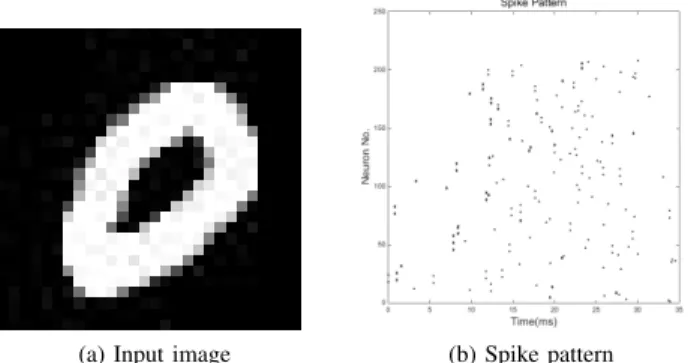
(a) Input image (b) Spike pattern
Fig. 4: Input image and its spike pattern generated from the first two layers.
pattern will contribute its part to the final learning efficacy matrix with certain selectivity.
Vthr=k∗max(V(t)) (8)
whereVthr is the post-synaptic potential threshold andV (t)
represents dynamic voltage. max (V (t)) is the maximum value of dynamic voltage within the predefined spiking time window and k (0.8 in this paper) depicts a positive constant within the range[0,1].
Through spiking encoding layer, the local invariance fea-tures will be transformed into spike trains. Fig.4 shows one input image and its spike pattern after processing with the first two layers. Such spike trains can be considered as a spike pattern. Therefore, each input image will generate its own unique spike pattern through the first two layers. Such spike pattern contains specific spatiotemporal structural information about its input image and thus the selectivity to this specific input image has been emerged. Ideally, at least from the learning method’s perspective, one can expect that those spike patterns generated from the same class would somehow looks similar to each other, while spike patterns from vary classes would be significantly different.
C. Output Layer
The whole visual pattern recognition framework contains two important parts:spike pattern generatingandspike pattern learning. According to modified rank order coding scheme, the former one generates spike pattern based on the local invariance features. While the latter one uses unsupervised STDP learning rule to learn the generated spike pattern and thus obtained the final synaptic efficacy matrix with certain selectivity. Notably, the next input image should feed into the feed-forward spiking neural network only until the current input image has been successfully trained or tested. After successfully learning the current input image, the intermediate variables generated during the training procedure will be reset to default values, except for the learning efficacy matrix.
1) Structure of the output layer: This layer includes several neurons and the total number of neurons is the same as the total classes. The neurons within spiking encoding layer
and output layer are fully connected so that each output neuron receive synaptic connections from all the neurons within spiking encoding layer. The output layer is the only learning layer in the proposed feed-forward spiking neural network. From above two layers, the spike pattern associated with the input image will be generated and such spike pattern conveys certain selectivity to its input image. Specifically, the spatiotemporal information embedded within the spike pattern plays an important role in defining such selectivity. The learn-ing method within output layer should fully investigate such spatiotemporal information and thus use the learning results to distinguish the testing samples. Spike-timing-dependent plas-ticity (STDP) learning rule has been employed to the output layer and it will dynamically changes the synaptic efficacy according to the learning window. Eventually, the synaptic efficacy matrix will be stabilized and thus the selectivity will be emerged after the learning procedure. The output layer uses winner-take-all strategy so that the first fired neuron will strongly depress the rest neurons within the output layer from firing spikes and thus the input image will be considered as the class associated with the fired neuron. So there are lateral depression connections appears in the last layer.
2) STDP Learning Rule: Hebb’s postulate [23] may be the most important theory in neuroscience trying to explain the adaptation of neurons in the brain during the learning process. It can summarized as ”Cells that fire together, wire together”. This kind of statement emphasize the causality between pre and post-synaptic neurons. Hebb emphasized that cell A needs to take part in firing cell B, and such causality can only occur if cell A fires just before, not at the same time as, cell B.
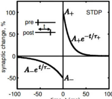
Spike-timing-dependent plasticity (STDP) [7], [8], [9], [10], [11] has been proved to be a quiet effective learning rule by neuroscientists, which adjusts the efficacy of synaptic connections based on the relative timing of post-synaptic spike and its input pre-synaptic spike. Like Hebb’s postulate, it also emphasizes the causality between pre and post-synaptic neu-rons. Actually, it can be considered as a temporally asymmetric form of Hebb’s rule. In neuroscience, long-term potentiation (LTP) is a persistent strengthening of synapses based on recent patterns of activity, while long-term depression (LTD) is an activity-dependent long-lasting reduction in the efficacy of neural synapses. When a pre-synaptic spike fires slightly earlier than the post-synaptic spike, the associated synap-tic efficacy will be potentiated (LTP). While the associated synaptic efficacy will be depressed (LTD) if the pre-synaptic synaptic spike fires later than the post-synaptic spike. The STDP function W (t) can be expressed as follows (t is the time difference between pre and post-synaptic spikes):
W(t) =A+exp −t τ+ f or t >0 (9) W(t) =−A-exp t τ f or t <0 (10) where A+ andA- represent amplitude of LTP part and LTD part of the learning window, respectively. τ+ andτ- are time constant for LTP and LTD, respectively. For biological reasons,
Fig. 5: STDP learning window.
Fig. 6: Random examples of MNIST database.
it is desirable to keep the synaptic efficacy in a predefined range. Thus, a soft bound strategy [24], [25] has been used to ensure the synaptic efficacy remains in the desired range
wmin < wj < wmax. Fig.5 shows one example of STDP
learning window.
III. EXPERIMENTALRESULTS ANDANALYSIS MNIST handwritten digital characters database [26] is a well known benchmark in pattern recognition field. It contains 60000 training samples and 10000 testing samples (all sample size is28×28). It includes 10 classes that is digital handwritten digits from 0 to 9. Fig.6 shows some examples of MNIST database. It can be seen that the database has large intra-class variance, which could be a real challenge for the proposed method. For instance, the digit 1 and 7 in Fig.6 have different external shape (the fifth digit in the second row and the sixth digit in the last row have significant different external shape compared with other samples in their class). Sometimes, even human being cannot easily recognize some digits of the database. For example, the fifth digit in the last row could be seen as 4 or 6 and each one can have their own opinion. Therefore, by testing the performance using this MNIST handwritten digital characters database, one can conclude the advantages and limitations of the proposed SNN and its own unsupervised learning method.
A. Parameter Setting
Before elaborating the experimental results, the experimen-tal parameter settings using in the SNN is needed to state first. All parameters are chosen from biologically plausible range and have been optimized to achieve its optimum state. The time resolution of this experiment is 0.1ms. In this paper, for the S1 and C1 features of the feature extracting layer, we used the same parameter setting as the HMAX model. The only difference is that only first 2 scales are used in the experiment.
For spiking encoding layer, we use a linear equation and the specific absolutely C1 feature values to generate the spikes. For the leaky integrate-and-fire model used in output layer, the
αfunction described in equation (6) has been used to mimic the time course of the dynamic synaptic current and the time constantτ used in the equation is set to 2.5ms. Equation (7) was used to compute the dynamic synaptic voltage, where the initial condition Vr is 0, the membrane time constant is 10
ms and the resistance R is 0.1 mΩ. The absolute refractory period is set to 1 ms. For STDP learning of the output layer, the time constant τ+ and τ- are set to 0.0168 and 0.0337, respectively. For soft bound strategy, the maximum weight and the minimum weight are set to 1 and 0, respectively.
B. Experiments and Discussions
Ideally, we expect that there are little intra-variance or even no intra-variance existed in the extracted features. However, such critical need cannot easily be satisfied. In the following subsections, we will discuss how STDP learning can handle the senarios with no intra-variance and large intra-variance, respectively.
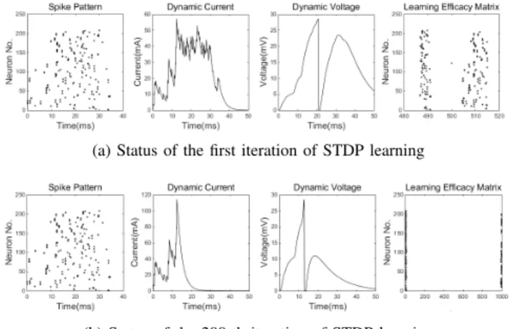
1) STDP Learning with no Intra-class Variance: Fig.7 shows dynamic learning procedure of generating selectivity after using unsupervised STDP learning method. Fig.7 (a) shows the beginning of the learning procedure. It can be seen that the dynamic synaptic current fluctuates over the whole time window and the synaptic voltage reaches its threshold at about 21ms. The synaptic efficacy weights are relatively random at this stage. After presenting the same input image (same input image in Fig.4) to the SNN system about 300 times, the selectivity finally emerged, just as the Fig.7 (b) shows. At this stage, the synaptic current only fluctuates over the first half time window and the synaptic voltage fires the spike at about 13ms. Whats more, the synaptic efficacy matrix has a special status with most weights take 0 and the rest take 1 [12]. Therefore, the selectivity to this specific input image emerges. However, such learning results can be generated only if the intra-class variance of the input images remains at a reasonable level.
2) STDP Learning with Relatively Large Intra-class Vari-ance: In Fig.7, an ideal experimental condition that the input image with no intra-class variance has been tested with the proposed timing-based feed-forward spiking neural network and obtained an ideal STDP learning efficacy matrix. However, in real world, such ideal condition is hardly achieved as vast intra-class variance existed among the samples. In this paper, we proved that certain selectivity to the input can be learned using unsupervised STDP learning rule even If the intra-class variance level of the input remains at a relatively high level, as shown in fig.8 (a),(b),(e),(f).
In Fig.8, two groups with two input images have been used to learn the selectivity using unsupervised STDP learning rule. In fact, input images (a) and (e) are the same. The group one uses (a) and (b) as its input images, (c) and (d) represent dynamic efficacy matrix of 20-th and 200-th iterations, respectively. (e) and (f) have been fed into group
(a) Status of the first iteration of STDP learning
(b) Status of the 200-th iteration of STDP learning
Fig. 7: Generating selectivity by using unsupervised STDP learning. The resolution for learning efficacy matrix (x axis) is set to 0.001 so that the maximum value equals to 1.
two, and thus obtained its 20-th and 200-th dynamic efficacy matrix, shown as (g) and (h). Here, one iteration means sequentially fed the two input images into the feed-forward spiking neural network one by one. From Fig.8, one can easily concluded that training samples with more intra-class variance will somehow hard to learn the selectivity. In other words, the dynamic efficacy matrix can be very hard to concentrate on the extreme values of 0 and 1 if having high level of intra-class variance within the training samples. Compared to the same input image (a), input image (f) is much more different than the input image (b), thus the dynamic efficacy matrix of group two had more weights lingering between the extreme values of 0 and 1.
Fig.9 shows the dynamic learning procedure using the proposed SNN and its STDP learning rule for one class. It is worth to note that one iteration in this experiment means sequentially feed 50 different training samples within certain class one by one. From Fig.9, it can be seen that the dynamic status only have a very limited changes. However, even the intra-class variance in the experiment remains at a relatively high level, the training samples are not totally independent (totally random samples), and thus such seemingly random learning efficacy matrix may contains certain selectivity to the input. Therefore, one question still need to answer that is how many iterations does the experiment need to achieve the optimum performance.
3) Experiments on MNIST Database: In order to answer the above question, by using the proposed unsupervised STDP learning rule, we randomly choose 50 different training sam-ples for each class and 100 different testing samsam-ples to test the correct classification rate. In the following experiment, each test follows the same procedure mentioned above. To be fair, each iteration within each test uses the same randomly chosen training samples and testing samples.
Table.I shows the corresponding correct classification rate performance when using the experimental conditions men-tioned above. Average correct classification rate also has been
(a) (b)
(c) (d)
(e) (f)
(g) (h)
Fig. 8: (a) and (b) are input images of group one, (c) and (d) are dynamic efficacy matrix of 20-th and 200-th iterations, respectively; (e) and (f) are input images of group two, (g) and (h) are dynamic efficacy matrix of 20-th and 200-th iterations, respectively. The resolution for learning efficacy matrix (x axis) is set to 0.001 so that the maximum value equals to 1.
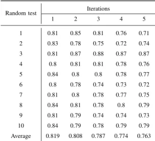
added in the table. It can be seen that all correct classification rates using one iteration, besides random test1 and test3 , are larger than others using different iterations. Even though the correct classification rates in these random tests are not so smooth, one can still easily estimate the performance range that is from 0.7 to 0.9. Besides, only using STDP learning with one iteration means the processing time will dramatically de-crease compared with others using more iterations. Therefore, from the above observation and analysis, one can conclude that only one iteration can be ensured to get the optimum correct classification performance. The final expected correct classi-fication rate can be obtained by averaging the classiclassi-fication
(a) The first iteration (b) The 5-th iteration
(c) The 10-th iteration
Fig. 9: Learning efficacy matrix with large intra-class variance. The resolution for learning efficacy matrix (x axis) is set to 0.001 so that the maximum value equals to 1.
TABLE I: Correct classification rate using differ-ent iterations for 10 random tests.
Random test Iterations
1 2 3 4 5 1 0.81 0.85 0.81 0.76 0.71 2 0.83 0.78 0.75 0.72 0.74 3 0.81 0.87 0.88 0.87 0.87 4 0.8 0.81 0.81 0.78 0.76 5 0.84 0.8 0.8 0.78 0.77 6 0.8 0.78 0.74 0.73 0.72 7 0.81 0.8 0.78 0.77 0.75 8 0.84 0.81 0.78 0.8 0.79 9 0.81 0.79 0.74 0.74 0.73 10 0.84 0.79 0.78 0.79 0.79 Average 0.819 0.808 0.787 0.774 0.763 •Note: 0.81 in this table means 81% correct classification
rate.
performance of those 10 randomly tests. Therefore, with only one iteration, 82% correct classification rate can be obtained if using the proposed SNN and its unsupervised STDP learning rule. Since the random training samples contain relatively large intra-class variances, increasing the iteration times may have somehow decreased the data correlation between samples within the same class. This could be one possible explanation for such behavior observed in our experiments. Table.II shows
TABLE II: Experimental running time(s). Period The Whole running time Running time per step
Training 23.32 0.047
Testing 5.63 0.056
•Note: The whole training procedure includes 500 steps for the total 10 classes (50 steps for each class) and the whole testing procedure includes 100 steps.
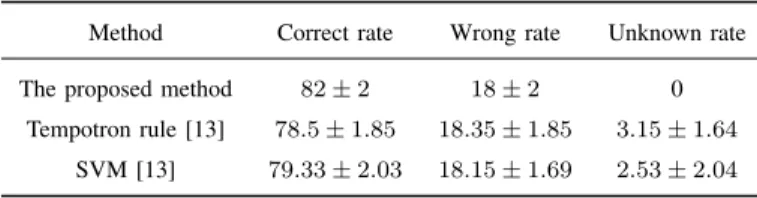
TABLE III: Performance comparison of three methods(%). Method Correct rate Wrong rate Unknown rate
The proposed method 82±2 18±2 0 Tempotron rule [13] 78.5±1.85 18.35±1.85 3.15±1.64
SVM [13] 79.33±2.03 18.15±1.69 2.53±2.04
the experimental running time of the whole procedure and each training step for training and testing period, respectively. It can be seen that the proposed method is not time-consuming and quite capable of on-line learning.
In paper [13], the authors used a supervised temporal learning rule (named Tempotron Rule) to train the MNIST database (almost same experimental conditions as this paper) and achieved 79% correct classification rate in the end. Unlike this state-of-art learning method, the proposed algorithm uses unsupervised STDP learning rule with dynamic post-synaptic potential threshold during the learning procedure. Dynamic post-synaptic potential threshold guarantees that each training sample will be properly learned. Table.III shows the final clas-sification performance comparison of three different methods. The parameters used in Tempotron rule and classical SVM method can be found in paper [13]. It can be seen that the unknown rate of the proposed method is 0, which means each testing sample would be recognized as one possible class. Compared with Tempotron Rule, the proposed method achieves better correct rate at around 82%, while still remains slightly less wrong rate.
IV. CONCLUSION
In this paper, equipped with LIF neuron model, a spike timing-based feed-forward spike neural network and its own unsupervised STDP learning rule with dynamic voltage thresh-old have been proposed. Satisfactory experimental results have been achieved on classic MNIST hand written digit database. It has been shown that the proposed SNN and its STDP learning rule can still learn certain selectivity about the input even it has large intra-class variance. Such advantage is extremely useful for the real time visual pattern recognition tasks. Compared with traditional visual pattern recognition algorithms, the proposed algorithm is a bio-inspired method with great potential. Even the coding scheme of brain is still largely unknown, the proposed method could be added to the further understanding of the dynamic processing procedure existed in brains V1 and V4 areas.
REFERENCES
[1] S. Thorpe, D. Fize, and C. Marlot, “Speed of processing in the human visual system,”Nature, vol. 381, no. 6582, pp. 520–522, 1996. [2] W. Gerstner and W. M. Kistler,Spiking neural models. Cambridge,
MA: Cambridge University Press, 2002.
[3] F. Rieke, R. Warland, D.de Ruyter van Steveninck, and W. Bialek,
Spikes:Exploring the neural code. Cambridge, MA: MIT Press, 1996. [4] M. N. Shadlen and W. T. Newsome, “Noise, neural codes and cortical
organization,”Curr. Opin. Neurobial., vol. 4, pp. 569–579, 1994. [5] W. Gerstner, “Population dynamics of spiking neurons: fast transients,
asynchronous states and locking,”Neural Comput., vol. 12, pp. 43–89, 2000.
[6] N. Brunel, F. Chance, N. Fourcaud, and L. F. Abbott, “Effects of synaptic noise and filtering on the frequency response of spiking neurons,”Phys. Rev. Lett., vol. 86, pp. 2186–2189, 2001.
[7] W. Gerstner, R. Kempter, J. L. van Hemmen, and H. Wagner, “A neuronal learning rule for sub-millisecond temporal coding,” Nature, vol. 386, pp. 76–78, 1996.
[8] R. Kempter, W. Gerstner, and J. L. van Hemmen, “Hebbian learning and spiking neurons,”Phys. Rev. E, vol. 59, pp. 4498–4514, 1999. [9] H. Markram, J. Lubke, M. Frotscher, and B. Sakmann, “Regulation of
synaptic efficacy by coincidence of postsynaptic aps and epsps,”Science, vol. 275, pp. 213–5, 1997.
[10] G. Q. Bi and M. M. Poo, “Synaptic modifications in cultured hip-pocampal neurons: dependence on spike timing, synaptic strength, and postsynaptic cell type,”J Neurosci, vol. 18, pp. 10 464–10 472, 1998. [11] P. J. Sjstrm, G. G. Turrigiano, and S. B. Nelson, “Rate, timing, and
cooperativity jointly determine cortical synaptic plasticity,” Neuron, vol. 32, pp. 1149–1164, 2001.
[12] T. Masquelier, R. Guyonneau, and S. J. Thorpe, “Spike timing dependent plasticity finds the start of repeating patterns in continuous spike trains,”
PLoS ONE, vol. 3, no. 1, p. e1377, 2008.
[13] Q. Yu, H. Tang, K. Tan, and H. Li, “Rapid feedforward computation by temporal encoding and learning with spiking neurons,”IEEE Trans. Neural Networks and Learning Systems, vol. 24, no. 10, pp. 1539–1552, 2013.
[14] S. Thomas, W. Lior, B. Stanley, R. Maximilian, and P. Tomaso, “Robust object recognition with cortex-like mechanisms,” IEEE Trans. Pattern Anal. Mach. Intelli., vol. 29, no. 3, pp. 411–426, 2007.
[15] T. Masquelier and S. J. Thorpe, “Unsupervised learning of visual features through spike timing dependent plasticity,”PLoS Computational Biology, vol. 3, no. 2, p. e31, 2007.
[16] Y. Bengio, “Learning deep architectures for ai,”Found. Trends Mach. Learn., vol. 2, no. 1, pp. 1–127, 2009.
[17] Y. Bengio, A. Courville, and P. Vincent, “Representation learning: A review and new perspectives,”IEEE Trans. Pattern Anal. Mach. Intell., vol. 35, no. 8, pp. 1798–1828, 2013.
[18] T. Serre, M. Kouh, C. Cadieu, U. Knoblich, G. Kreiman, and T. Poggio, “A theory of object recognition: Computations and circuits in the feedforward path of the ventral stream in primate visual cortex,” 2005. [19] T. Christian, T. Nicolas, and C. Matthieu, “Extended coding and pooling in the hmax model,”IEEE Trans. Image Processing, vol. 22, no. 2, pp. 764–777, 2013.
[20] A. Delorme, J. Gautrais, R. van Rullen, and S. Thorpe, “Spikenet: a simulator for modeling large large networks of integrate and fire neurons,”Neurocomputing, vol. 26, pp. 989–996, 1999.
[21] A. Delorme, L. Perrinet, and S. Thorpe, “Networks of integrate-and-fire neurons using rank order coding,”Neurocomputing, vol. 38-40, pp. 539–545, 2001.
[22] A. Delorme and S. Thorpe, “Face identification using one spike per neuron: resistance to image degradation,”Neural Networks, vol. 14, no. 6-7, pp. 795–803, 2001.
[23] D. O. Hebb,The Organization of Behavior: a neuropsychological theory. New York: Wiley, 1949.
[24] M. C. W. van Rossum, G. Q. Bi, and G. G. Turrigiano, “Stable hebbian learning from spike time dependent plasticity,”Journal of Neuroscience, vol. 20, no. 88, pp. 12–21, 2000.
[25] J. Rubin, R. Gerkin, G. Bi, and C. Chow, “Calcium time course as a signal for spike-timing-dependent plasticity,”J Neurophysiol, vol. 93, pp. 2600–13, 2005.