CHARACTERIZING INCOME DISTRIBUTION FOR POVERTY AND INEQUALITY ANALYSIS *

CHARACTERIZING INCOME DISTRIBUTION FOR

POVERTY AND INEQUALITY ANALYSIS

*

RÓMULO A. CHUMACERO† RICARDO D. PAREDES‡

* _{We thank Felipe Balmaceda, Osvaldo Larrañaga, Claudio Montenegro, Jaime Ruiz-Tagle,}

and Arístides Torche for helpful comments and suggestions. Yolanda Portilla provided able research assistance. The usual disclaimer applies.

† _{Department of Economics of the University of Chile and Research Department of the}

Central Bank of Chile. E-mail: rchumace@econ.uchile.cl

‡ _{Escuela de Ingeniería, Pontificia Universidad Católica de Chile. E-mail: rparedes@ing.puc.cl} Abstract

This paper presents a systematic empirical characterization of income distribution in Chile. Such characterization helps us to understand the apparent paradox regarding the coexistence of a successful economic performance and persistently high inequality in income distribution and to assess the impact of different social policies dealing with poverty. Segmented sectors seem to be a crucial feature that is generally overlooked in the traditional analysis of income distribution and poverty. As an example, we conduct an exercise to evaluate two types of policies used to alleviate poverty: one focused on increasing coverage of education (wrongly assuming a single population), another in reducing the quality gap (rightly assuming two populations).

Resumen

Este trabajo es una caracterización empírica sistemática de la distribución de ingresos en Chile. Esta caracterización permite entender la aparente paradoja por la que coexisten resultados económicos exitosos y una desigual y persistente distribución. Una característica empírica de relevancia generalmente ignorada es la de segmentación. Como un ejemplo, el trabajo muestra los potenciales efectos de políticas que pretenden disminuir la desigualdad: una que pretende incrementar la cobertura educacional (asumiendo erróneamente una población homogénea) y otra que pretende reducir la brecha en calidad de la educación (asumiendo poblaciones heterogéneas).

JEL Classification: C14, C15, C24, D31, D63, I32, J16.

1. INTRODUCTION

Different studies suggest that Chile has one of the most unequal income distributions in the world (see, for instance, Wold Bank, 1997 and 2000). Despite a relatively rapid reduction of poverty, Gini coefficients and other measures of income inequality have remained persistently high over the years. This persistence, and more importantly, the high inequality, have been accompanied by a good economic performance, well developed institutions to help the poorest, and a relatively recognized educational system (see, Mideplan, 1999; Beyer, 1999; Cowan and De Gregorio, 1996; and Valdés, 2002).

Three stylized facts characterize the recent Chilean experience. First, income distribution, measured by different statistics, has remained virtually unchanged over time, and particularly, over the most dynamic period in Chilean history, going from 1990 to 1998 in which GDP grew over 7% per year. The Gini index in 1990 was the same in 1998 (0.58) and the income ratio between last and first quintile was of 14.0 in 1990 and 15.5 in 1998. Second, income distribution in Chile is more unequal than in otherwise comparable countries, showing largest Gini indexes than East Asia, the Middle East and North Africa (0.38), and even the South Saharan Africa (0.47). Third, poverty has been reduced consistently (the incidence of indigence and poverty felt from 14.3% and 39.4% in 1987 to 4.9% and 19.7% in 1996).

Even though these facts are widely accepted (Labbe and Riveros, 1985; Cowan and de Gregorio, 1996; Beyer, 1997; Larrañaga, 1994; Ruíz-Tagle, 1999), there is less clarity on the nature and origin of such inequality; and hence, the policies best suited to reduce it. The analysis of poverty has focused mainly on its quantification, providing little insights on its causes. Only recently, there are more studies using panel information for less developed economies (See, Jalan and Ravallion, 1998; and Baulch and Hoddinott, 2000). In Chile, some recent studies using a panel data are shedding some light on the dynamics of poverty. However, the panel has only one wave and considers a short period (5 years), so most basic questions about the dynamics remain unsolved. Furthermore, whilst some studies (e.g., Contreras et al, 2004 and Zubizarreta, 2005) show more mobility than even some developed countries, an important proportion of people do not move and an important proportion of the poorest remained poor over the years.

Regarding policy implications, an important concept is that of “social exclusion” (associated with poverty levels that make it difficult for some individuals to participate in activities that are accepted as welfare enhancing), or hard or structural poverty. However, social exclusion does not come from a rigorous analytical framework. Nevertheless, this avenue of research may have helped to stress the importance of considering individual heterogeneity, both in econometric practice and in social program evaluation.1

In this paper we characterize the income distribution and poverty in Chile to derive policy implications. In particular, we are interested on testing whether a good statistical representation of the income distribution can provide evidence of the presence of different populations, different returns to human capital and

1 _{As Heckman (2001) and Heckman and Vytlacil (2001) put it, accounting for individual}

different effects of alternative social policies in the line suggested by the literature related with structural poverty. We focus our analysis in the year 1996, which is representative of the period where Chile experienced its longest and biggest economic expansion (1985-1997).

The paper is organized as follows: Section 2 develops traditional statistical characterizations of the unconditional distribution of income. Section 3 discusses how the usage of alternative econometric techniques can help us to uncover key characteristics of the unconditional distribution that can not be captured using the methods discussed on Section 2. In Section 4 we explore alternative representations for the conditional distribution. Section 5 uses the results obtained previously to evaluate the effects of alternative types of policies on income distribution and poverty. Section 6 concludes.

2. INCOME DISTRIBUTION

2.1. Unconditional Analysis

This section provides an empirical characterization of the unconditional distribution of income among households. Our approach is progressive, in the sense of building up on parametric and nonparametric approximations to the unconditional density. To this end, we analyze income distribution in Chile in 1996 by using the National Socioeconomic Characterization Survey (CASEN), which is a cross sectional survey with detailed information on employment, housing, health, and income. The survey was applied to 33,617 households from a universe of approximately 3.6 million households.

We define the following variables of interest: total income of household i

(denoted by Hi), per-capita income of household i (denoted by Yi=Hi/ni, where ni

is the number of members of the household) and, y_i is the (natural) logarithm of Y_i. Table 1 presents basic summary statistics for these variables. The average monthly income of a household was of US$1,066 with a median income of US$597. On the other hand, the average monthly per-capita income was of US$270 with a median of US$145. As can be noticed, these variables are highly dispersed, given that their coefficients of variation (Standard Deviation over Mean) exceed unity. As usually happens with the series in levels, and consistent with the fact that the average income of a household is substantially lower than the median income, there is strong evidence of departures from normality, presenting in both cases (H and Y) a positive skewness and excess of kurtosis.

Table 1 also displays an estimate for the Gini indexes (G) and their associated standard deviations. The standard deviations were obtained through weighted bootstrapping.

As Park and Marron (1990) and Wand, et al. (1991) make clear, the choice of bandwidth is critical. In our case, if we use the bandwidth proposed by Silverman (1986) we obtain a smooth density that appears to have different characteristics from the density that is obtained from, say, half its size (Figure 1).2 _{A feature that}

2 _{It is important to mention that most of the statistical software that have kernel density}

TABLE 1 DESCRIPTIVE STATISTICS H_i Y_i y_i Mean 1066 270 5.052 Median 597 145 4.979 Standard Deviation 1717 473 0.981 Skewness 8.359 [0.000] 12.104 [0.000] 0.219 [0.000] Kurtosis 158.201 [0.000] 355.786 [0.000] 4.201 [0.000] Jarque-Bera [0.000] [0.000] [0.000] Gini 0.541 (0.006) 0.551 (0.007)

Notes: Standard deviations in parenthesis. P-values in brackets. The standard deviations for the Gini coefficients were computed using weighted bootstrapping over 1,000 artificial samples.

FIGURE 1

UNCONDITIONAL DISTRIBUTION OF H_i (KERNEL ESTIMATOR)

0.0000 0.0002 0.0004 0.0006 0.0008 0.0010 0.0012 500 1000 1500 2000 2500 3000 Kernel -1.5E-07 -1.0E-07 -5.0E-08 0.0E+00 5.0E-08 1.0E-07 500 1000 1500 2000 2500 3000 h/2 h 3h/2 Second Derivative

distinguishes both densities is that the one estimated with h/2 has at least a distinct “bump” and may even be bimodal while the one obtained with h does not have these characteristics. Bimodal densities for income distribution are well documented in the literature and a choice of bandwidth that over-smooths the estimated density may not be able to capture it.

Once nonparametric estimates of the unconditional densities are obtained, we evaluate some familiar parametric counterparts, in particular, density functions that have a non-negative domain. To provide a guide of our progress with respect to which specification is preferred by the data, we report the Akaike Information Criterion (AIC).

Our initial search specializes on densities that are unimodal and thus do not seem to match a characteristic that appears to be important if we take into account the results that were obtained from the nonparametric estimates. The main findings for both H and Y are that when confronted with the data; of all the densities considered, a lognormal approximation renders the best results.

Nevertheless, even if we ignore for the moment the bimodality that appeared to be present in the nonparametric estimation, a lognormal approximation (which is unimodal) has the property of being completely characterized by the two parameters estimated. In particular, using both parameters we can estimate the mean, median, mode, skewness and kurtosis implied by the lognormal approximation.3 _{However, this parametric alternative does not fully capture} important regularities of the series. Thus, even though we find that the parameters estimated are able to replicate the first moments (medians, modes and means), in both cases they substantially underestimate the coefficient of variation, skewness and kurtosis.

That led us to turn our attention to providing a good statistical description for y. Given that y can now take any value on the real line, we look for parametric densities that conform to this domain.

3 _{See Evans, et al. (1993) for details.}

TABLE 2

ALTERNATIVE DENSITIES FOR y_i

Distribution AIC Parameters

Location Scale Shape

Generalized Cauchy 1.387 5.026 (0.001) 2.541 (0.003) 4.853 (0.009) Error 1.399 5.048 (0.001) 0.937 (0.001) 1.034 (0.001) Extreme Value 1.527 4.579 (0.001) 1.090 (0.001) Laplace 1.412 4.979 (0.005) 0.755 (0.001) Logistic 1.388 5.020 (0.001) 0.543 (0.001) Normal 1.588 5.052 (0.001) 0.981 (0.001) Student’s (Noncentral) T 1.387 5.026 (0.001) 0.742 (0.001) 8.705 (0.019) Notes: AIC = Akaike Information Criterion. Standard deviations in parenthesis.

Table 2 and Figure 2 report these results. An interesting feature of these results is that, even though the “best” parametric alternative for modeling Y was the lognormal distribution, corresponding to y being normal. When confronted with other parametric alternatives (such as the Generalized Cauchy, Student’s T, and to a lesser extent the Logistic distribution), the normal distribution does the poorest job on fitting the data. The most successful approximations (such as the Logistic or the Student’s T) are able to capture the leptokurtic characteristics of the data. However, with the sole exception of the Extreme Value distribution, all the others are symmetric and thus do not capture the marginal evidence of positive skewness reported on Table 1. Furthermore, all of the distributions considered are unimodal, and though a few of these alternatives resemble the shape of the kernel estimate, they do not display the apparent bimodality that once again arises.4

FIGURE 2

ALTERNATIVE DENSITIES FOR y_i

4 _{Given that the unconditional moments of y and Y differ in important respects (such as the}

attenuated excess of kurtosis and positive skewness) the caveats for choosing the bandwidth of the kernel estimator are not present in this case. In fact, the test graph method showed that Silverman’s suggestion for h was now, if anything, undersmoothing the estimated pdf.

0.0 0.1 0.2 0.3 0.4 0.5 -2 0 2 4 6 8 10 0.0 0.2 0.4 0.6 0.8 -2 0 2 4 6 8 10 0.0 0.1 0.2 0.3 0.4 0.5 -2 0 2 4 6 8 10 0.0 0.1 0.2 0.3 0.4 0.5 -2 0 2 4 6 8 10 Cauchy Error Kernel Extreme Value Laplace Kernel Student’s T Kernel Logistic Normal Kernel

2.2. Conditional Analysis

Given the previous results, we pursued the matter of possible bimodality on the unconditional pdf of y using parametric and seminonparametric alternatives that do not constraint our search to unimodal representations. This section develops two alternative estimates for the density of y by using more complex econometric techniques that, in principle, can represent it better.

The first builds on the increasingly popular approach of modeling time series which is commonly referred to as Markov Switching Regime Models (see Hamilton, 1994 or Kim and Nelson, 1999). In our case we will focus our attention to processes known as i.i.d. mixture distributions. The second that, to our knowledge, has never been used before in this context combines the estimation of truncated densities with threshold models. For completeness, we first provide a brief description of each of the techniques used, reporting their results immediately after.

i) Mixture of Distributions

One way to approximate relatively intricate density functions is by means of mixing i.i.d. distributions. It is well known that even simple mixtures of normal distributions can generate rather complex pdfs (see Hamilton, 1994 for a few examples). In our case, given that y can, at least in principle, take any value on the real line, we will approximate its pdf by mixing independent normal distributions. Briefly, we assume that there are J possible states or regimes. Associated with each of them there is a pdf. The econometrician observes realizations of a random variable x, but can not associate each observation with the pdf that generated it. That is because for every observation x_i, there is a latent random variable si that determines from which regime that observation was generated.

For every observation i, s_i can take the value of 1,2,..,J. When the process is in regime j (si=j), the observed variable xi is presumed to have been drawn from a

N(μ_j, σ_j). Hence, the density of x_i conditional on the random variable s_i=j is:

f xi si j x j i j j | = ,

(

)

= ⎛ − μ ⎝ ⎜ ⎞_⎠⎟ θ σ φ σ 1

ø (·) where corresponds to the pdf of a standard normal.

The unobserved regime is presumed to have been generated by a probability distribution, for which the unconditional probability that si takes on the value of

j is denoted π_j. According to this setup, it can be verified (Hamilton, 1994) that the unconditional density of xi is:

(1) f xi jf xi si j j J |θ π | ,θ

(

)

(

=

)

=

∑

1

Once the unconditional density is found, the likelihood function can be constructed and the parameters involved estimated by conventional numerical methods.5

5 _{The parameters to be estimated are the means and standard deviations of the J normal}

An interesting feature of this type of models is that we can conduct inference about which regime was more likely to have been responsible for producing the observation x_i. In this case, we have:

(2) Pr | , | , | s j x f x s j f x i i j i i i =

(

)

=

(

=

)

(

)

θ π θ θ

Thus, one can obtain estimates of these probabilities by replacing the Maximum Likelihood estimator of θ. We applied this methodology allowing for several values of J.

ii) Truncation and Thresholds

As Deaton (1998) points out, at least for the case of developing countries, attention is often focused less on inequality and income distribution than on poverty. One of the main features that characterize this literature is the construction of poverty lines and headcount ratios.

Poverty lines are usually constructed resorting to some arbitrary procedure that includes a type of threshold. One says that a person or a household is poor when its income is below this threshold, while if the contrary is true, that person is labeled as non-poor.

This line provides a threshold that considers one population to be the complement of the other (see e.g. Kakwani, 1980 or Deaton, 1998). The problem with this approach is that if we were to use this principle in any meaningful way, we have to adopt a stance with respect to precisely where that threshold should be.

In our case, we define the threshold l as the income that maximizes the differences between two populations in a specific metric. The difference with the standard practice is that this threshold is formally estimated and has confidence intervals that can be assigned to it.

Threshold models have a long-standing tradition in econometrics and are frequently used in time series (see e.g. Hansen, 1997 and references therein). A crucial difference between that literature and our application is that in our case, the threshold variable is the same one that we are describing. In particular, assume that we consider that all the observation of a variable x that are below a given threshold l belong to one population, and its complement to another. Belonging to different populations must imply, in this context, that there are different pdfs associated with each. Given that the threshold variable is also x we must ensure that all the observations up to the threshold can not be characterized by the other distribution. In this context, thresholds imply truncated distributions.

If we denote by f

( )

⋅ and f

( )

⋅ as the pdfs with truncation from above and below respectively and we impose the assumption of normality, we have:

(3) f x x l f x x l x l f x x l f x x l x l | Pr / / | Pr / / ≤ ( )= ( ) ≤ ( )= − μ

(

)

(

)

− μ

(

)

(

)

> ( )= ( ) > ( )= − μ

(

)

(

)

−

(

(

− μ

)

)

(

)

φ σ σ σ φ σ σ σ 1 1 1 1 2 2 2 21 2 2 Φ Φ

For a given value of l, can be optimized using conventional numerical methods by estimating the parameters that characterize f

( )

⋅ and f

( )

⋅ separately. An estimator of l can then be obtained by maximizing

(4) lˆ arg w I l l f x x| l I l l f x x| l l L i i N i i =

[

( ) ( ) ( ≤ )+

(

− ( )

)

(

− ( )

)

( > )

]

∈ ∑= max n 1 1 π 1 1 π

where I_i

( )

⋅ is an indicator function that takes the value of 1 when xi≤l and 0

otherwise; and (5) π l w I l w i i i N i i N

( )

= =

( )

=

∑

∑

1 1

is introduced in order to scale the unconditional pdf of x. As the optimization of can be numerically intensive, a direct search can be applied for a grid of l given that it is naturally spanned by the values of y.

If poverty lines have any empirically meaningful content, _lˆwould provide a data driven estimate. We can then evaluate if this dichotomy accommodates the data better than other alternatives.

iii)Results

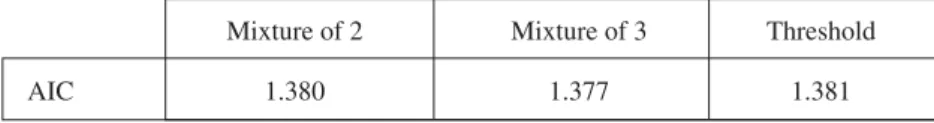
Table 3 and Figure 3 report the results for the specifications we estimated.

TABLE 3

ALTERNATIVE DENSITIES FOR y_i

Mixture of 2 Mixture of 3 Threshold

AIC 1.380 1.377 1.381

Notes: Mixture of j denotes a mixture of j normal distributions. The threshold estimator for l that maximized was 4.4 (approximate US$82).

For the case of the mixtures of normal distributions up to 4 distributions were allowed; while not reported, only marginal improvements were obtained with mixtures of 4 normal distributions. Finally, for the case of the threshold estimation, was estimated by direct search (see Figure 3).6

6 _{Figure 3 also reports the results of estimating the unconditional density of y using the}

SNP (Semi Nonparametric) estimation technique developed by Gallant and Nychka (1987) and Gallant and Tauchen (1998). Its main advantage is that it provides a flexible functional representation for the density function.

Our main findings are two. First, while mixtures of 2 and 3 normal distributions do a better job on tracking the kernel estimator than any univariate distribution previously considered, it is difficult to identify if there is more than one mode present on the data given that the distributions are close to each other. Second, even though the estimated threshold that dichotomizes two populations was obtained through a rigorous approach, this estimator does a very poor job approximating the unconditional distribution of y.7

Recalling that mixture models allow us to conduct inference about which regime was more likely to have been responsible for producing a given observation, we applied together with the estimates reported in Table 4 to obtain the conditional probabilities of Figure 4. When a mixture of 2 normal distributions is considered, and given that the parameters associated with the first state have higher mean and variance, extreme observations (low and high income levels) are associated with s=1. This reassures our previous finding in the sense of not favoring a clear-cut separation of the population solely based on income. Even though the results for the case of a mixture of 3 normal distributions distinguish 3 “populations”, once again the factor that discriminates one from the others can not be disentangled based on income alone.

Concluding, commonly used parametric alternatives for characterizing the unconditional distribution of y are easily outperformed by models that allow for mixtures of distributions, while there is no evidence that income alone can help us separate populations from different distributions.

FIGURE 3

ALTERNATIVE DENSITIES FOR y_i

0.0 0.1 0.2 0.3 0.4 0.5 0.6 -2 0 2 4 6 8 10 SNP Truncated Threshold Kernel 0.0 0.1 0.2 0.3 0.4 0.5 -2 0 2 4 6 8 10 Mixture of 2 Normals Mixture of 3 Normals Kernel

7 _{The last column of Table 4 reports the parameters estimated for the threshold process; as}

can be observed, when the density is truncated from above, the only way to fit the data is by inflating the first two moments of the truncated normal.

3. INCOME DISTRIBUTION: CONDITIONAL ANALYSIS

The previous sections provided empirical characterizations of the unconditional distribution of y, which displays strong departure from normality and the possible existence of more than one mode. It may be correctly argued that these features can be easily explained once we consider what are the determinants of the level of income. For example bimodality in the unconditional distribution can be introduced if there are two groups of individuals that have one characteristic that difference them. This can be shown, for instance, from the relationship between income and schooling. Assume that there are two types of individuals, those that finished high school and those that did not. If the log of the level of income for individual i is given by:

(6) yi = +α βSi+εi

TABLE 4

PARAMETERS ESTIMATED WITH ALTERNATIVE DENSITIES FOR y_i

Mixture of 2 Mixture of 3 Threshold

s=1 s=2 s=1 s=2 s=3 s=1 s=2

μ 5.32 4.84 4.30 4.76 5.64 60.70 4.50

σ 1.21 0.68 1.75 0.70 1.03 5.44 1.25

π 0.44 0.56 0.03 0.62 0.35

Notes: All the parameters reported are statistically significant at conventional levels. The parameters reported for the case of the threshold estimation correspond to a value of l equal to 4.4 (approximately US$ 82).

FIGURE 4

CONDITIONAL PROBABILITIES FOR MIXTURES

1.0 0.8 0.6 0.4 0.2 0.0 1.0 0.8 0.6 0.4 0.2 0.0 -2 0 2 4 6 8 10 -2 0 2 4 6 8 10 Pr(s=1) Pr(s=2) Pr(s=1) Pr(s=2) Pr(s=3)

where S adopts the value of 1 if the individual finished high school and 0 otherwise, and e is a Gaussian disturbance, one can obtain bimodality and important departures from normality on the unconditional distribution of y if β≠0.8 _{The same kind of} argument can be used for any other variable that has an influence on the determination of y and that has the property of exclusion. In fact, this is precisely the argument used by Deaton (1998) to motivate bimodality on the unconditional distribution of y for the case of South Africa (relating S to race.)

The main characteristic of this line of argument is that for instance, the presence of more than one mode on the unconditional distribution can be attributed to some observable variable, and that this feature can be uncovered once we control for it. We take issue with this explanation and present the results for a conditional analysis of income distribution. To do so, we first show some characteristics of variables that are commonly used as “determinants” of the level of income.

8 In this case, it is not sufficient to have a value of β that differs from zero, but that _{S itself}

must not be unimodal.

FIGURE 5

Figure 5 presents the kernel estimate of the joint pdf of y and the level of education of the head of the household (measured by years of schooling).9 _At least two features of this estimate are worth noting. First, conditional on a particular level of income, more than one mode for the years of schooling appears to be present. As y is positively correlated with years of schooling, at least in principle, more than one mode on the unconditional distribution of y can be attributed to this characteristic. Second, while not as evident, for several years of schooling (i.e. controlling by schooling), there also appears to be more than one mode in y.

Table 5 presents a quantified cross tabulation between gender and years of schooling. That is, for each combination of Gender and Education we computed the average level of monthly per capita income and its coefficient of variation.10 As expected, a higher level of education of the head of the household is associated with higher average incomes and, at least for the totals, lower relative dispersion. On the other hand, there is no clear-cut association between gender and income, given that for low levels of education (less than 6 years of schooling) the average per capita income in households with a female head is significantly lower than in households with a male head. Nevertheless, this gap is reversed for all the other levels of education. As we will reaffirm later, studies that tend to suggest a causal relationship between income and gender may be missing the point completely (e.g. Mideplan, 1999).

9 _{If not noted otherwise, the variables used in our conditional analysis refer to observations}

for the head of the household. While not reported, results obtained with other variables such as the average or the maximum value of a characteristic for a household are similar.

10 _{For example, the average monthly income for a person that lived on a household that had}

a female head with less than 6 years of schooling was of US$148.

TABLE 5

QUANTIFIED CROSS-TABULATION

Education Male Female Total

Less than 6 169 (2.001) 148 (1.024) 163 (1.844) Between 6 and 12 213 (1.362) 238 (1.312) 217 (1.355) More than 12 644 (1.376) 674 (1.294) 648 (1.365)

Total 273 (1.773) 255 (1.627) 270 (1.751)

Notes: Values in parenthesis correspond to the coefficients of variation.

Consistent with the above, if we focus on traditional measures of inequality (such as Lorenz curves or Gini coefficients) we observe that the distribution of income among households with male or female heads is undistinguishable from the distribution on the total. This is not the case for households with different years of schooling (Table 6). In particular, income distribution is less egalitarian

for households with higher education, which in turn appears to be more heterogeneous particularly since the early 1980s (see, Robbins, 1995).

Given that there are systematic factors (such as education) that are closely related to the level of income of a household, Table 6 reports the results of estimations for the conditional density of y.

To analyze the “determinants” of the level of income, several characteristics of the unit were regressed with y. The second column of Table 6 presents the

FIGURE 6

LORENZ CURVES (GENDER AND EDUCATION)

0.0 0.2 0.4 0.6 0.8 1.0 0.0 0.2 0.4 0.6 0.8 1.0 0.0 0.2 0.4 0.6 0.8 1.0 0.0 0.2 0.4 0.6 0.8 1.0 Male Female Total 45° Less than 6 Between 6 and 12 More than 12 Total 45° TABLE 6 CONDITIONAL DISTRIBUTION OF y_i

No Mixture Mixture of 2 Mixture of 3

s=1 s=2 S=1 s=2 s=3 Constant 4.358 4.452 3.943 4.417 4.456 3.148 Gender -0.103 -0.149 0.129 -0.103 -0.145 0.616 Schooling 0.090 0.080 0.133 0.048 0.107 0.120 σ 0.884 0.751 1.300 0.613 0.863 1.757 π 1.000 0.822 0.178 0.371 0.591 0.038 AIC 1.296 1.282 1.276

Notes:π = Unconditional probability of belonging to a state. All the variables are statistically at a 1% level.

results of an exercise of this nature. In contrast to the results of Table 5 where we found that on the aggregate households with female heads had significantly lower per capita incomes, Table 6 shows that after controlling by schooling, the coefficient associated with gender (1=Male, 0=Female) is negative and statistically significant. In turn, the return to an additional year of schooling is of 9%.11

We also estimated models in which we allowed for conditional mixtures of distributions. As Table 6 makes evident, mixture models are preferred to models in which only one state is considered. More importantly, in both the cases of 2 and 3 mixtures, statistically different returns for years of schooling were found for each regime.12 _{In particular, in the case of 2 mixtures, the return of one more} year of schooling for households in the second state is 5% higher than for those in the first. These differences are even more important if a mixture of 3 distributions is considered. It is also important to notice that the coefficient associated with gender varies depending on the state. After controlling by schooling, there is still (marginal) evidence that unconditionally (with respect to the regime) households with female heads earn more their male counterparts. Also, the distributions with higher returns to schooling are also associated with greater dispersion. If we consider, for example, the mixture of 3 distributions, the standard deviation of the innovations of the third regime more than doubles the standard deviation of the other two.

The existence of a mixture of distributions suggests some sort of segmentation. Given that even after controlling for other observed variables we still find evidence of mixtures, it could be suggested that some other unobservable variable that presents some sort of bimodality may have been omitted. However, variables such as ability, beauty, race, health and others we may think of are not expected to display that feature for the case of Chile. In this sense, the explanation behind the mixture of distributions that we observe may be found on the labor literature on segmentation (e.g. Dickens and Lang, 1985; Basch and Paredes, 1996). This argument is valid not only for labor market regulation but also, as suggested by Harberger (1971), it can be applicable to regulation in education, where focusing on the supply may promote segmentation.

The results of Table 6 can also be applied to obtain similar results than those found in Figure 4. While not reported, it is not difficult to anticipate that for any given level of education, it is more likely that households with lower income belong to states of lower return to schooling. This suggests that policies that are aimed to increase the level of schooling of the poor may not be as desirable as policies that increase their return. The next section describes a simple exercise that can help us to quantify the magnitude of these effects.

11 _{While not reported, several other characteristics such as age (both linear and quadratic)}

and years of experience on the job were also included.

12 _{This is possibly a reason why non-linear terms of years of schooling (such as quadratic}

terms) may appear as statistically significant when no mixtures are allowed. In the case of mixtures, there is a natural interpretation for different returns of schooling, while increasing returns in the case of no mixtures is difficult to justify but easy to obtain when the true process is generated from mixtures.

4. POLICY IMPLICATIONSFROM TWO SCENARIOS

Mixtures of distributions better characterize the conditional distribution of income than any alternative with no mixtures. The consequences for distribution and poverty policies are important if, as it is likely, behind these distributions there are elements that make unlikely for a person in one distribution, to move to the other one. Thus, policies would affect differently depending upon the regime to which a given household belongs. For instance, if we consider the results obtained with mixtures of 3 distributions, one additional year of mandatory schooling would increase the household per capita income in 4.8%, 10.7% and 12.0% depending on the regime a household belongs to.13 _{In turn, if} the unobservable state s reflects “quality” of education (or any other non directly controlled variable, like belonging to the primary or secondary sector), we can evaluate the social effects on a household of moving from, say, the first regime to the second compared with moving through the same regime.

In what it follows, we conduct two experiments that are intended to shed some light regarding the effect of policies aimed at reducing poverty and inequality. In the first, we consider increasing the minimum years of schooling of the head of the household. In the second, we consider some policy that shift people from a low segment to a better one. For purposes of clarity, we associate this policy to an improving of the quality of education for households with low returns. In turn, the dimensions on which the effects of these experiments are evaluated are two: first, we provide an approximation for the valuations of each policy by part of the households themselves; and second, we discuss the possible effects of these experiments on income inequality.

Even when these exercises may be considered as crude approximations, they are valuable because they do not only provide insights with respect to which type of “policies” would be preferred by the households, but also on the nature of the phenomenon of persistently high inequality that is present in Chile. First consider increasing the minimum years of schooling that every head of household has. Assume that household i has X_i as its vector of characteristics; if this household belongs to regime j, its expected income is given by:

(7) _{E Y X s}

(

_{i| i, i} =_j

)

=_eβjXi+0 5.σj

2

where are the coefficients associated with regime j that were reported on Table 6.14 _{Given that s is unobservable, we can compute the “unconditional”} expectation of as follows: (8) E Y Xi i jE Y X si i i j j J | | ,

(

)

=

(

=

)

=

∑

π 1

Let _Xim _{be the vector of characteristics X of household i with the caveat that} if that household has less than m years of schooling, that characteristic is replaced by m on X. If the household head had more schooling than m, _Xim_{and X}

i coincide.

13 _{In the year 2002 it was enacted a law that increased mandatory education from 8 to 12 years.} 14 _{Lognormality of Y was imposed in order to compute.}

In either case, we define the “unconditional” expected income for household i

when m is set as the minimum years of schooling as:

(9) E Y Xi i E Y X s j m j j J i i m i | | ,

(

)

=

(

=

)

=

∑

π 1

Denoting by Am _{to the average valuation of a policy that increases the}

minimum years of schooling to m we obtain:

(10) A w E Y X E Y X w m i i i m i i i N i i N =

(

)

⎡ ⎣⎢ ⎤⎦⎥−

(

)

= =

∑

∑

| | 1 1

and apply for several values of m.

The second experiment consists on improving the state the person is. The effect of such policy is evaluated by increasing the return to education, while leaving the years of schooling unaffected. We led this exercise to the extreme case in which the probability of observing si=J is set equal to 1. That is, all the

individuals in the population have the same returns to schooling (returns of the last regime). In this case, the average valuation of such a policy (B) is given by:

(11) B w E Y X s J E Y X w i i i i i i i N i i N = =

[

(

=

)

−

(

)

]

=

∑

∑

| , | 1 1

Equations and provide a simple way to compare the valuation that the “average” household would have for each policy. The results of such a comparison are reported in Figure 7.

FIGURE 7

VALUATIONS OF ALTERNATIVE POLICIES (MONTHLY PER CAPITA US$)

0 200 400 600 800 1000 1200 10 15 20 25 m Mixture of 2 0 200 400 600 800 1000 1200 10 15 20 25 m Mixture of 3 A B A B

The average valuation of the experiment aimed to increase the return of schooling is equivalent to an increase of US$246 and US$355 on the monthly per capita income on the average household, depending on whether a 2-regime or a 3-regime mixture is considered. These figures are substantial, and at least for the case of a mixture of 3 normal distributions implies a valuation that exceeds the average per capita income of the households reported in Table 1 (US$270). At any rate, the values of m that would make the average household indifferent between the first and second experiments are 16.5 and 18.5 respectively, which would roughly be equivalent to having every head of household having finished college or having been graduate students. In other words, it seems clear that

Another exercise that was also conducted refers to how inequality would be affected by each experiment. For that purpose we device a Monte Carlo experiment in which 1,000 artificial samples were generated. Each sample had 1,000 households that were drawn randomly in direct proportion to the distribution of characteristics of the population (years of schooling, gender, etc). Each household (with its characteristics) was then randomly assigned to a given regime according to the probabilities reported on Table 6. A realization of per capita income was then drawn using a random realization of a standard normal together with the vector of characteristics attributed and the parameters estimated for the corresponding regime.

Once an artificial sample (with 1,000 households) was generated, we computed its Gini index. For each artificial household generated, we also applied the two experiments previously described. Care should be taken in this case, as for the exercise to be meaningful, the Gaussian random realization corresponding to the innovation on income has to be the same when an experiment is applied and when it is not. For the case of the experiment that increases the minimum years of schooling, we set m=12 and m=16.

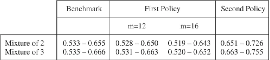
Table 7 reports the 95% empirical confidence intervals for these Monte Carlo experiments. We want to remark two results. First, even unrealistically important changes in m associated with the first experiment provide only slight and marginally significant improvements on the Gini index. In fact, for all the cases analyzed, the 95% confidence intervals include the point estimate of the Gini index reported on Table 1 (0.551). This means, that policies that focus on

TABLE 7

GINI INDEXES FOR ALTERNATIVE POLICIES (95% CONFIDENCE INTERVALS)

Benchmark First Policy Second Policy

m=12 m=16

Mixture of 2 0.533 – 0.655 0.528 – 0.650 0.519 – 0.643 0.651 – 0.726 Mixture of 3 0.535 – 0.666 0.531 – 0.663 0.520 – 0.652 0.663 – 0.755 Notes: This Table reports 95% confidence intervals for Gini indexes computed from alternative policies. Benchmark = No policy is carried out. All the figures were constructed from Monte Carlo realizations of 1,000 artificial samples of households. The 95% empirical confidence intervals correspond to the 25th _{and 975}th _{sorted Gini indexes.}

increasing the level of schooling without modifying its quality are not only less valued by the households, but also have only second order effects in terms of diminishing inequality. Second, popular policies such as increasing mandatory schooling produce the unambiguous result of increasing inequality. This result is easy to explain; once we realize that the last regime in every mixture does not only have the higher return to years of schooling but also a substantially higher variance.

5. CONCLUDING REMARKS

In this paper we provided a systematic empirical characterization of income distribution in Chile by using flexible forms. We found that mixtures of distributions performed better than simple parametric alternatives, feature that is consistent with the literature on labor markets that suggest that segmentation and exclusion may be behind the determinants of income in Chile. In particular, we found more than one population with different returns to human capital.

This finding may not only call for additional efforts to characterize income dispersion than is possible through the use of traditional indexes (such as Gini and Theil), but also provide insights on the most effective directions for policies aimed at reducing poverty and income inequality. The success of targeted policies is substantially reduced when it is difficult to identify the population from which a family showing an income just below a given level comes from. For instance, the impact of policies that reduce the “unexplained gap” of populations, such as improving the quality of education or increasing the years of schooling, will have a very different effect depending on the benefited population.

We performed two exercises that may be associated with policies that reduce the gap of populations (e.g., improving the quality of education) and policies affecting the number of years of schooling. We conclude that focusing on policies that reduce heterogeneity, like improving the quality of education, is more valued and effective in reducing poverty than increasing its quantity. However, such a policy does not imply a reduction in inequality and, on the contrary, may increase it. Second, policies traditionally followed in Chile to deal with poverty, like increasing mandatory schooling, may have an extremely low effect on reducing income inequality.

REFERENCES

Basch, M. and R. Paredes (1996). “Are Dual Labor Markets in Chile?: Empirical Evidence”.Journal of Development Economics 50, 297-312.

Baulch, B. and J. Hoddinott (2000): “Economic Mobility and Poverty Dynamics in Developing Countries”, The Journal of Development Studies, August 2000: 1-24.

Beyer, H. (1997). “Distribución del Ingreso: Antecedentes para la Discusión”. Estudios Públicos, Nº 65.

Contreras, D., R. Cooper, J. Herman and C. Neilson (2004): “Dinámica de la Pobreza y Movilidad Social: Chile 1996-2001”, Universidad de Chile, Departamento de Economía.

Cowan, K. and J. de Gregorio. (1996). “Distribución y Pobreza en Chile: ¿Estamos Mal? ¿Ha Habido Progresos? ¿Hemos Retrocedido?”. Estudios Públicos, Nº 64.

Deaton, A. (1998). The Analysis of Household Surveys: A Microeconometric Approach to Development Policy. The Johns Hopkins University Press. Dickens, W. and K. Lang (1985). “A Test of Dual Labor Market Theory”.

American Economic Review 75, 792-805.

Evans, M., N. Hastings, and B. Peacock. (1993). Statistical Distributions. John Wiley & Sons.

Gallant, R. and D. Nychka. (1987). “Semi-nonparametric Maximum Likelihood Estimation”. Econometrica 55, 363-390.

Gallant, R. and G. Tauchen. (1998). “SNP: A Program for Nonparametric Time Series Analysis”. Manuscript. Duke University.

Hamilton, J. (1994). Time Series Analysis. Princeton University Press. Hansen, B. (1997). “Inference in TAR Models”. Studies in Nonlinear Dynamics

and Econometrics 2, 1-14.

Harberger, A. (1971). “On Measuring the Social Opportunity Cost of Labor”. International Labor Review 103, 559-579.

Heskia, I. (1980). “Distribución del Ingreso en el Gran Santiago 1957-1979” Working Paper Nº 53, October, Department of Economics, University of Chile.

Heckman, J. (2001): “Microdata, Heterogeneity, and the Evaluation of Public Policy”, Nobel Lecture in Economics, Journal of Political Economy. Heckman, J. and E. Vytlacil (2001): “Policy-Relevant Treatment Effects”,

American Economic Review, 107-11.

Jalan, J. and M. Ravallion (1998): “Determinants of Transient and Chronic Poverty: Evidence from Rural China”, Banque Mondiale.

Jalan, J. and M. Ravallion (2000): “Is transient poverty different? Evidence for rural China”, in Economic mobility and poverty dynamics in developing countries. (Baulch B. & Hoddinott J. eds.): 82-99; Frank Cass Publishers. Kakwani, N. (1980). Income Inequality and Poverty: Methods of estimation

and Policy Applications. Oxford University Press.

Kim, C. and C. Nelson. (1999). State-Space Models with Regime Switching: Classical and Gibbs-Sampling Approaches with Applications. The MIT Press.

Labbe, F. and L. Riveros. (1985). “Distribución del Ingreso en Santiago”. Revista Economía y Administración, Facultad de Ciencias Económicas, U. De Chile, Santiago, Chile.

Lanjouw, J. (1997). “Behind the Line: Desmystifying Poverty Lines”, in Poverty Reduction. Module 3. Poverty Measurement: Behind and Beyond the Poverty Line, New York, UNDP.

Larrañaga, O. (1994). “Pobreza, Crecimiento y Desigualdad: Chile 1987-92”, Revista de Análisis Económico 9, 69-92.

Mideplan. (1999). “Situación de la Mujer en Chile: Resultados de la VII Encuesta CASEN 1998”. Working Paper 11. Mideplan.

Pagan, A. and A. Ullah. (1999). Nonparametric Econometrics. Cambridge University Press.

Park, B. and J. Marron. (1990). “Comparison of Data-Driven Bandwidth Selectors”. Journal of the American Statistical Association 85, 66-72.

Ravallion, M. (1994): Poverty Comparisons. Fundamentals of Pure and Applied Economics, Chur, Switzerland: Harwood Academic Publishers. Robbins, D. (1995). “Wage Differences and Comparative Advantages”, Estudios

de Economía, Santiago, Chile

Ruiz-Tagle, J. (1999): “Chile: 40 Años de Desigualdad de Ingresos”, Working Paper N° 165, Departamento de Economía Universidad de Chile, November. Silverman, B. (1986). Density Estimation for Statistics and data Analysis.

Chapman & Hall.

Valdés, A. (2002). “Pobreza y Distribución del Ingreso en una Economía de Alto Crecimiento: El Caso de Chile 1987-1998”, Report 22037-CH. The World Bank.

Wand, M., J. Marron, and D. Ruppert. (1991). “Transformations in Density Estimation”. Journal of the American Statistical Association 86, 343-353. World Bank (1997): “Chile. Poverty and Income Distribution in a High-Growth

Economy: 1987-1995”, Report 16377-CH. The World Bank.

World Bank. (2000): “The Nature and Evolution of Poverty”, Manuscript. The World Bank.

Zubizarreta, J.M. (2005): “Dinámica de la Pobreza en Chile”, Thesis, Escuela de Ingeniería, Pontificia Universidad Católica de Chile.