Efficient Viewshed Computation Algorithms On GPUs and CPUs

University of South Florida University of South Florida

Scholar Commons

Scholar Commons

Efficient Viewshed Computation Algorithms On GPUs and CPUs

Efficient Viewshed Computation Algorithms On GPUs and CPUs

Faisal F. Qarah

University of South Florida

Follow this and additional works at: https://scholarcommons.usf.edu/etd Part of the Computer Sciences Commons

Scholar Commons Citation Scholar Commons Citation

Qarah, Faisal F., "Efficient Viewshed Computation Algorithms On GPUs and CPUs" (2020). Graduate Theses and Dissertations.

Efficient Viewshed Computation Algorithms On GPUs and CPUs

by

Faisal F. Qarah

A dissertation submitted in partial fulfillment of the requirements for the degree of

Doctor of Philosophy in Computer Science and Engineering Department of Computer Science and Engineering

College of Engineering University of South Florida

Major Professor: Yicheng Tu, Ph.D. Adriana Iamnitchi, Ph.D. Yan Zhang, Ph.D. Zhuo Lu, Ph.D. Joni Downs, Ph.D. Date of Approval: June 19, 2020

Keywords: Computing visibility, GPU, GIS, Parallel algorithm, Spatial data analysis Copyright c 2020, Faisal F. Qarah

Dedication

Dedicated to the memory of my father, Fawzi Qarah, who never gave up on me and encouraged me to accomplish my achievements.

Acknowledgments

First and foremost thanks to ALLAH, the Almighty,and the greatest of all, for giving me the opportunity, the determination, and the strength to do my research and complete this dissertation.

I would like to thank my mother, my brothers, my sister, and my friends for their endless support, patience, and encouragement over the years while I laboriously worked on my dissertation. Also, special thanks to my daughter, Ameera, for all the joy and happiness she brought to me.

I would like also to thank my dedicated advisor, Dr. Yicheng Tu, for his guidance and encouragement in this graduate research work. He spends a lot of time and effort to support me in both academic and non-academic matters. His insights at times helped me whenever I faced a difficulty.

I am also grateful to the committee members, Dr. Adriana Iamnitchi, Dr. Joni Downs, Dr. Yan Zhang, and Dr. Zhuo Lu, who express interest in this work and offered their valuable time throughout this dissertation.

Special thanks to the management and administration at the main office, Department of Computer science and engineering USF, for their help in supplying the necessary documents and aid in other matters.

Finally, I am grateful to Taibah University for supporting me financially and granting me this scholarship for studying Ph.D. at the University of South Florida.

Table of Contents

List of Tables iii

List of Figures iv

Abstract vii

Chapter 1: Introduction 1

1.1 Terrain Representation 1

1.2 Visibility Problem Definition 3

1.3 Contributions 4

Chapter 2: Literature Review 6

2.1 RSG-Based Viewshed Analysis Algorithms 6

2.1.1 R3 Algorithm 7

2.1.2 R2 Algorithm 7

2.1.3 Radial sweep algorithm 9

2.2 TIN-Based Viewshed Analysis Algorithms 12

2.3 Overview of GPU Architecture 14

Chapter 3: The Proposed Algorithms 17

3.1 Parallel radial-sweep algorithm on GPU 17

3.2 Optimizing Memory Utilization 23

3.2.1 The CPU-Based Optimized Algorithm 24

3.2.2 The GPU-Based Optimized Algorithm 25

Chapter 4: Evaluation and Results 32

4.1 Parallel GPU-based radial-sweep Algorithm 33

4.2 The efficiency of using static BST 35

4.3 Memory-optimized radial-sweep algorithm 37

4.4 Optimizing the Merge-sort (MergePath) Algorithm 42

Chapter 5: Conclusion and Future Work 49

5.1 Conclusion 49

Appendix A: Copyright Permissions 54

List of Tables

Table 4.1 Description for the data used in Section 4.1, and obtained from [27]. 33 Table 4.2 Performance results for original implementation (VT=11, NT=256) vs.

new implementation (VT=22, NT=128) on a list of size 100M elements

List of Figures

Figure 1.1 Two DEM representations. (a) is an illustration for RSG data model,

(b) is an illustration for TIN data model [10]. 2

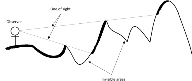
Figure 1.2 An illustration of the line-of-sight where the invisible areas are blocked

by other areas with higher elevation-slope. 4

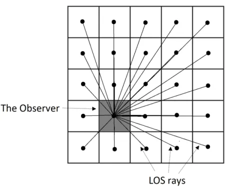
Figure 2.1 An Example of R3 algorithm where it computes the visibility of every cell individually by launching a line-of-sight to all surrounding cells. 8

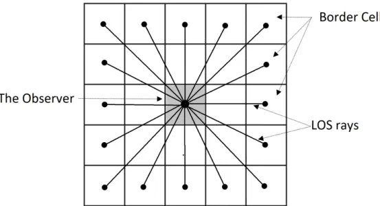
Figure 2.2 Illustration for R2 algorithm, where it launches LOS rays from the ob-servation point to all border cells, and while these rays are advancing, they compute the visibility of the internal nodes the came across. 9

Figure 2.3 Insert and remove events locations. There are 8 main regions, and in

every region the events position varies. 13

Figure 2.4 An example of the radial-sweep algorithm and the rotating-line ap-proach. Highlighted cells are active cells that are currently intersecting

with the sweeping line. 13

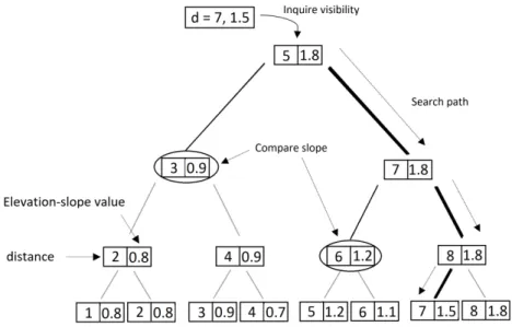
Figure 2.5 Example of the status-tree structure. There are two types of nodes: leaf nodes which contain active cells’ information, and internal nodes that contain the highest elevation-slope value stored in their children. During an “inquire visibility” operation, when the search-path takes the right direction, it compares the target-cell elevation-slope with the value

stored in the left-child. 14

Figure 3.1 An example of the mergePath approach when dividing the merge op-eration between two threads, the cross-diagonal value determines how many elements each thread can fetch from each subarray. In this exam-ple, the first thread will fetch 3 elements from A and 4 elements from B (total = 7), and the second thread will fetch the remaining elements (4

from A and 3 from B) [25]. 20

Figure 3.2 An illustration of building a histogram and then applying prefix-sum operation on it so each thread can identify the starting index of its

partition in the event-list. 21

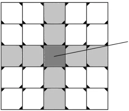
Figure 3.3 Dividing the grid into 4 or 8 scan-regions to facilitate searching cell IDs

in a target sector. 26

Figure 3.4 A grid with 8 scan-regions that has been divided into 10 sectors. Some

sectors are located over two scan-regions. 27

Figure 4.1 Comparing all already known exact-viewshed algorithms with our GPU-based parallel radial-sweep algorithm using a grid size of (10800 x 10800).

34

Figure 4.2 Comparing all exact-viewshed algorithms using different datasets. 35 Figure 4.3 The break-down of execution time for GPU-based radial-sweep

algo-rithm stages taken from the first experiment 36

Figure 4.4 The break-down percentage of the I/O portion and the computation portion of the overall execution for parallel radial-sweep on GPU 36 Figure 4.5 Showing the efficiency of using a static BST in building the status-tree

instead of the conventional status-tree built using a dynamic BST over different data sizes. The new approach improved performance by up to

44x. 37

Figure 4.6 Comparing memory requirement for the status-tree for two CPU-based sequential radial-sweep. The first algorithm used the conventional dy-namic BST, and the second used the new static BST. The experiment shows the new status-tree requires 70% to 80% less memory based on

Figure 4.7 The execution time of two variations of the new optimized CPU-based radial-sweep algorithm when dividing the data into a different number of sectors using a data size of (25K x 25K). The first variation search for cell IDs in a target sector by scanning a “full quadrant”. While the second variation searches for cell IDs by scanning a “half quadrant”. The experiment shows both variations maintain the same performance as the original algorithm when dividing the grid into 12 or fewer sectors. Also, the algorithm based on the “half quadrant” search-region shows significantly better performance when dividing the data into a large number of sectors. The “original” case refers to our static-BST-based radial-sweep algorithm without any segmentation. 41 Figure 4.8 Measuring the performance of all three exact-viewshed algorithms over

data in different sizes. The original GPU-based radial-sweep algorithm

cannot process data larger than (10K x 10K). 42

Figure 4.9 Algorithm-5 A high-level abstraction of the MergePath algorithm on

GPU. 43

Figure 4.10 Illustration on how to combine the workload of two threads to be

exe-cuted by only one thread. 46

Figure 4.11 Combining the workload of multiple threads to be executed by only one

thread. 47

Figure 4.12 The execution time of the original and the optimized MergePath

Abstract

Nowadays with the advance in managing and collecting large data, GIS is one of the applications that suffer from lack of efficient data management methods. GIS data often come in form of maps with different types of data such as temperature, topology, and pop-ulation. This dissertation focuses on exact-viewsheds computation for large terrains, and due to the poor performance of current exact-viewshed algorithms that may need several hours to process a midsize map, we found the need for new algorithms that are capable of efficiently computing viewshed for large size maps. This work presents a highly-efficient exact-viewshed computation algorithm based on the radial-sweep algorithm, implemented and optimized for GPUs. The first version of our GPU algorithm shows significant improve-ment in performance over the sequential CPU-based algorithm, providing at least an order of magnitude speedup.

We further improve the algorithms by tackling two challenges in parallelizing the radial-sweep algorithm: (1) dividing the elevation-grid into small-size sectors accurately between threads and (2) consumption of excessive amount of memory.

Both problems have been resolved in the newly proposed algorithms. We were able to parallelize the algorithm by building a histogram for cells’ events based on their azimuth-angle in the grid. The histogram we help each thread to know the number of events it has to process which forms a small size sector. Then, we applied prefix-sum operation on the histogram so each thread will know where to start processing the events. The second problem which is the excessive memory consumption has been resolved by dividing the grid

into sectors and processing them individually to obtain a smaller intermediate result instead of processing the whole grid that would yield a larger intermediate result. Also, to search for cell IDs in each sector, the grid is divided into scan-regions where the overhead of the scan operation is minimal. The new GPU-based algorithm is 4.4x faster than the fastest existing GPU-based exact-viewshed computation algorithm, and the new sequential CPU-based algorithm is 44x times faster than the current fastest sequential algorithm.

Chapter 1: Introduction

Viewshed computation is an important operation that is widely used in GIS, games, and simulation applications, such as locating critical facilities in a suitable location [1], plac-ing guards and watchtowers for security purposes [2], buildplac-ing media and communication networks [3] [4] [5], and monitoring environmental influences on properties values [6]. How-ever, current exact-viewshed algorithms are very time consuming compared to approximate-viewshed algorithms that are less accurate but more time-efficient. Thus, the main goal of this dissertation is to develop an efficient exact-viewshed algorithm that can be used in real-life applications. This can be achieved by designing a new algorithm for the graphical processing unit (GPU) that in recent years show a significant improvement in performance in many application domains.

1.1 Terrain Representation

In GIS, data that contains the elevation measurements for different regions in terrain are represented using the Digital Elevation Models (DEMs) [3], which contain the elevation measures for all cells in a 2-dimensional space. There are two different data models of DEM that are widely used in GIS: Regular Squared Grid (RSG), and Triangulated Irregular Network (TIN). RSG (also called elevation-grid, or raster-cells) (Fig. ??.a) is the simplest representation of the two models. Where the terrain’s surface is divided into square or rectangular cells of equal size, and a single elevation value is assigned to each cell where all points or pixels within that cell will share the same elevation value. Thus, DEM resolution [7]

Figure 1.1: Two DEM representations. (a) is an illustration for RSG data model, (b) is an illustration for TIN data model [10].

is determined by the number of length-meters a cell covers (e.g., if a cell represents an area of 10 x 10 meters then the DEM resolution is 10), and decreasing the size of the cell to obtain a better terrain representation will increase the resolution of the grid. TIN data model (Fig. ??.b) follows a different approach where different regions in the terrain are represented using a triangular plane (facet) of different sizes, and the elevation measures are stored in the vertices that compose the triangular planes. However, the vertices’ elevation values are not necessarily the same which means that points within the plane have different elevation measures. However, even though representing a terrain topology using TIN is more complicated than RSG, it does require significantly less memory space because it can represent a terrain using fewer planes and vertices [8]. Our research focus will be on viewshed computation algorithms designed for the RSG data model because it is preferred more in viewshed analysis [9]. Also, [10] compared computing viewshed between TIN and RSG and found that results obtained from analyzing viewshed using the RSG model are much more compatible with surveyed viewsheds in reality.

1.2 Visibility Problem Definition

The problem of computing viewshed or visibility analysis answers the question of which areas or regions are visible to a particular point of interest. That point is called the ob-servation point, and all surrounding points are called target-points. All points/cells in the elevation-grid holds an elevation value that shows the height for the area that the point or cell it covers [11] [12] [13] [14]. To check the visibility of a target point, the standard approach is to use what is called the line-of-sight (LOS) [1] which is a straight line that starts from the observation point and advances until it reaches the target-point (Fig. 1.2). In the meantime, the LOS keeps track of the greatest elevation-angle value it encounters by calculating it using equation (1.2) for every new point it passes by in its way. When the LOS reaches the target-point, it calculates its elevation-angle and compares it with the elevation-angle value it holds, if the new target point’s elevation-angle is greater than or equal the angle’s value the LOS has then the target-point is visible, otherwise it is considered invisible [1] [11] [14]. However, viewshed computations can be reduced if the elevation-slope value (using equation (1.1)) is used instead of the elevation-angle to determine the target-points visibility, which is a technique that has been used in previous literature such as [13]

CElevationSlope=

(hi−hpoi)

dvc

(1.1) Where hiis the height of cell c, hpoi is the height of point-of-interest v, and dvcis the distance

between v and c.

Figure 1.2: An illustration of the line-of-sight where the invisible areas are blocked by other areas with higher elevation-slope.

1.3 Contributions

In this dissertation, we present two new exact-viewshed computation algorithms that are considered to be the fastest in their class. The first algorithm is a parallel GPU-based algorithm, and the second is a sequential CPU-based.

Both algorithms are based on the original “Radial-sweep” viewshed computation algorithm that suffers from two main drawbacks: difficulty in parallelizing, and large memory consump-tion. Parallelization is an important feature for performance improvement, especially when targeting a massively parallel processing unit such as the GPU as the computing platform. The parallelization problem has been solved by using two parallel primitives: histogram and prefix-sum, which enable dividing the grid into small sectors, and each thread can know the starting index of its sector.

Resolving the memory consumption problem enabled both algorithms to significantly process much larger data. The strategy we used in solving this problem is by dividing the grid into equal-sized sectors and process them individually to obtain a smaller intermediate result instead of processing the whole grid that would yield a larger intermediate result. Also, to search for cell IDs in each sector, the grid is divided into scan-regions where the overhead of the scan operation is minimal. The experiment results show that segmenting the input data (elevation-grid) would add a small overhead to the new GPU-based algorithm, and no overhead at all to the CPU-based algorithm when dividing the grid into 30 sectors or less.

Also in this dissertation, we show the efficiency of using some of the novel optimization techniques used in the new algorithms such as using a static binary search tree instead of a dynamic tree in building the data structure that is responsible for handling the interme-diate results. Using the static BST in the GPU-based algorithm was crucial because of the difficulty of implementing dynamic data structures in GPUs’ algorithms, and our extensive study for the status-tree showed that the static BST is more suitable for the radial-sweep algorithm in general.

Finally, we present an optimization technique for the parallel merge-sort on GPU that is called “Merge Path” that ensures a more balanced workload between the running threads, which increases the sort performance by 8% on average and up to 17%.

Chapter 2: Literature Review

In recent years, many viewshed computation algorithms have been proposed that are different in terms of accuracy and time efficiency. In general, there are two types of viewshed algorithms: exact and approximate viewshed algorithms. Exact algorithms tend to produce highly accurate visibility results but suffer from poor performance, and on the other hand, approximate algorithms are time efficient but less accurate than exact algorithms [1] [15]. The research community’s main focus was on algorithms designed for the RSG model where both “exact” and “approximate” classes are been targeted. However, many have proposed different algorithms and approaches to analyze visibility for the TIN data model due to its wide use in GIS systems, but all TIN-based algorithms only approximating the visibility results due to the continuous nature of the TIN structure. Even though according to [16] the only commercial GIS software that offers computing viewshed for TIN maps is ESRI’s ArcGIS, but it first converts TIN to RSG and then computes the requested visibility query, which it shows the importance of developing more efficient viewshed algorithms designed for RSG data model.

2.1 RSG-Based Viewshed Analysis Algorithms

In this section, three of the most common RSG-based viewshed algorithms will be dis-cussed. R3 and radial-sweep algorithms fall under the “exact” viewshed class, and R2 is an approximation of R3.

2.1.1 R3 Algorithm

The first algorithm in computing viewshed is R3 [17]. It is considered to be the standard of all viewshed algorithms. It computes the POI’s viewshed by launching LOS rays from observation point v to every target cell located within sight range R (see Fig. 2.1). It was named R3 by [1] because, for range R, the execution time is R cubed. In other words, for an (n x n) grid and R = n, the time complexity for the algorithm is O(n3_{). In order to}

break down the time complexity for the algorithm, the grid size is n2_{, and it will compute}

the visibility for every cell in the grid. Every LOS will go through O(n) cells at most, or n/4 on average if the observation point is located in the middle of the grid. However, even though the algorithm is intuitive and very simple, it is considered to be the slowest of all viewshed algorithms.

The first GPU-based R3 algorithm was presented in [14], where they also consider the case when the elevation-grid does not fit in memory. The algorithm first divides the grid into tiles stored in host memory, and each tile consists of a group of cells. To ensure all necessary tiles are fetched within a single transfer from host to device, a preliminary processing phase is conducted to find all required tiles.

2.1.2 R2 Algorithm

[1] has proposed the R2 algorithm, which is an optimization for R3 and approximates the visibility results. Instead of launching LOS to every cell in the grid, it only launches LOS rays to border cells (Fig. 2.2), and they compute the visibility of every cell they encounter while advancing until they reach their final destination (i.e., border cells). Commonly, multiple LOS rays will encounter the same intermediate cell. Still, only one of them will conduct the visibility process, which is the one that considered being the closest to the center of the cell. Overall, the time complexity of the algorithm is O(n2), and hence this where it gets its

Figure 2.1: An Example of R3 algorithm where it computes the visibility of every cell individually by launching a line-of-sight to all surrounding cells.

name from. However, even though the algorithm is very time-efficient, it gives less accurate results yet often considered acceptable [1, 15].

[18] has proposed another I/O efficient algorithm for R2. The algorithm divides input data (elevation-grid) into blocks stored on disk. Whenever there is a need for a certain block, it will be fetched into memory using the LRU blocks management policy. [19] presented a pretty straightforward implementation for R2 on GPU, while [15] optimized R2 algorithm on GPU even further by utilizing the shared memory so consecutive threads can agree on which one of them is the most eligible for computing the visibility of a certain intermediate cell they all came across, and the elevation-grid is divided into horizontal segments in case the whole grid would not fit in global memory.

Figure 2.2: Illustration for R2 algorithm, where it launches LOS rays from the observation point to all border cells, and while these rays are advancing, they compute the visibility of

the internal nodes the came across.

2.1.3 Radial sweep algorithm

The second exact viewshed algorithm is called the radial-sweep or plane-sweep algo-rithm [11]. Its accuracy rate is equivalent to R3 [14], but it is more efficient. The algoalgo-rithm has adopted the sweeping-line approach presented in [20] for solving the “line segment in-tersection” geometric problem. The basic idea of the radial-sweep algorithm for computing viewshed is to rotate a straight line around the observation point sweeping all surrounding cells, and the rotating line completes a full round when rotating for 360◦. As the sweeping line is moving, it will trigger what is called an event every time it passes over a certain location within a cell (Fig. 2.3). Each cell has three different events: insert, inquiry, and remove. These events are managed using a special data structure called tree or status-structure which is an augmented balanced binary search tree that keeps track of all the cells that the sweeping line is currently crossing (Fig. 2.4). If the sweeping line came in contact with an insert event, which is the first point the sweeping line will pass over when it becomes

in contact with a cell, that cell information would be added to the status-tree. If the line passes over the remove event, the related cell information will be deleted from the status-tree. Finally, when the sweeping line intersects with the center of any cell, it will trigger an inquiry event, and hence it will check the visibility of that cell by applying search-like operation on the status-tree.

The status-tree is a special BST wherein its leaf nodes contain information about cells that are currently intersecting with the sweeping line (see Fig. 2.5). On the other hand, all internal nodes, including the root store the highest elevation-slope value that is available in its children nodes. This means the root node holds the highest elevation-slope value that is stored in all the leaf nodes. In order to process the visibility of a particular target-cell, the design of the status-tree helps to perform a search-like operation to obtain the target-cell visibility status efficiently. On the other hand, insert and remove operations become a little trickier where the elevation-slope values stored in the internal nodes would need adjustment especially if the cell that has been added or removed contains a relatively large elevation-slope value.

Leaf nodes in the status-tree are ordered by its distance from the observation point. Thus, distance d is considered to be the search key for the tree. Cells that are near the observer are located within the left subtree, and the farthest can be found in the right-subtree. Thus, the leftmost leaf node is the closest to the observation point, and the rightmost is the farthest. When comparing the complexity of different operations, it is safe to say that insert and remove operations are straightforward, while search (inquiry) operation, however, is a little trickier. When an inquiry event is triggered, it means we want to check the visibility of that cell by applying a search-like operation on the status-tree and by using the search key d, which is the cell distance from the observation point.

Starting from the root node, if the search path went toward the right sub-tree, it checks the elevation-slope value stored in the root’s left child. If the elevation-slope value is less

than the target cell’s slope, then the target cell is invisible, and the inquiry operation is terminated. Otherwise, the search process keeps going until it reaches the leaf node where target cell information is stored, which means it is visible to the observer because all slope-elevation values in every node on the left of the target cell are less than its slope value. The time complexity of the three operations on status-tree is similar to the same operations on a balanced binary search tree. The cost of each one of these operations O(log n) where the status-tree holds information for O(n) cells in any single moment. Also, the sweeping process itself would cost O(n2) because it is sweeping n2 cells and generating three events for each

cell. So total time complexity for the algorithm is O(n2_{log n). The algorithm is as follows:}

for every cell, generate all three events, and store them in the event-list. Sort the event-list in an ascending order based on the event’s azimuth-angle, distance from the observation point, and then by event-type (for events with the same azimuth-angle and distance values, delete events take the highest precedence, then inquiry events, and finally insert events). When all events are sorted, the algorithm starts fetching the events one by one and applies the appropriate operation associated with that event on the status-tree until processing all events in the event-list.

[13] has studied the radial-sweep algorithm and considered the case where the intermedi-ate results (event-list) does not fit in memory. Thus, they proposed the first I/O efficient radial-sweep algorithm based on the distribution sweeping approach [21]. They assume that the status-tree can be loaded into the memory, and the algorithm sorts and processes the event-list by streaming it from disk. In addition to the O(n2 log n) time complexity of the

original radial-sweep, the algorithm also requires O(sort(n2)) I/Os for sorting the event-list

on disk. However, our new optimized algorithm can resolve the issue of the event-list large size by using a much simpler yet efficient technique where all computations are conducted in-memory.

achieve such a goal, the elevation-grid is divided into multiple sectors equal to the number of CPU cores. However, the main challenge here is in finding all cells in each sector. Each core will search for target cells in its associated sector by applying an approach similar to the R2 algorithm, where it launches multiple straight lines from the observation point to border cells to search for all cells that might be located in-between. The search lines are adopting the DDA line drawing algorithm [22] to identify a possible new cell by calculating the new x-value and y-value of the farthest point in line with every step-increment.

After all cells have been identified, each core will apply the same original radisweep al-gorithm on its sector where each core will have its status-tree. However, using such an approach in order to search for cell’s IDs in each sector could reduce the overall accuracy of the algorithm if the search-lines skipped a cell when crossing its narrow corner, and the step-increment value is not small enough to catch that cell. In our proposed algorithm, we have used an alternative approach that efficient, yet it preserves the overall accuracy when parallelizing the computations.

2.2 TIN-Based Viewshed Analysis Algorithms

In contrast to RSG representation which is a discrete structure, TIN representation is more of a continuous structure. [3] presented a common approach called “front-to-back order” for computing visibility of TIN maps by adopting the continuous nature of the data. The algorithm basically starts processing planes that are closer to the observation point and then processing planes that are farther. However, the problem is in determining which triangular planes should be considered first where sorting the planes may not be achieved in all TIN maps except for TINs that are converted from RSG maps, and for non-sortable TINs, they adopted [23] approach for dividing the triangular planes into smaller triangles to make it sortable.

Figure 2.3: Insert and remove events locations. There are 8 main regions, and in every region the events position varies.

Figure 2.4: An example of the radial-sweep algorithm and the rotating-line approach. Highlighted cells are active cells that are currently intersecting with the sweeping line.

Figure 2.5: Example of the status-tree structure. There are two types of nodes: leaf nodes which contain active cells’ information, and internal nodes that contain the highest elevation-slope value stored in their children. During an “inquire visibility” operation, when the search-path takes the right direction, it compares the target-cell elevation-slope

with the value stored in the left-child.

when studying the difference in accuracy rate between RSG and TIN maps. In all four criteria, they started by generating a line-of-sight from the observation point to the target-triangle, and it would be considered visible based on the following criteria: if a point in the middle of the triangle is visible, if one of the vertices is visible, if two of the vertices are visible, or if all three vertices are visible. [24] did follow a different approach where a triangle is considered visible if all its three edges are visible to the observation point.

2.3 Overview of GPU Architecture

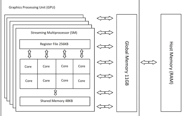
Because the new viewshed algorithm is designed for the Graphics Processing Unit (GPU) device, it is necessary to overview its general architecture briefly. There are multiple GPU devices in the market, but NVidia’s GPU devices and its programming model (CUDA) have been widely used by the research community compared to other brands. Despite the

fact that GPUs are designed to process games and video graphics, NVidia did present a new programming model that is called Compute Unified Device Architecture (CUDA) for general-purpose computing (GPGPU). Researchers and developers have been utilizing GPUs for solving different problems due to their massive computing power, and the high memory bandwidth the GPU provides. The general architecture for recent NVidia’s GPUs (see Fig. 2.6) is as follows: the GPU consists of multiple streaming multiprocessors (SM), where each one consists of multiple cores, a large register file, and a cache system. The GPU, in general, contains significantly more computing cores than the traditional

CPU. For example, Volta architecture contains 5120 cores distributed between 80 streaming multiprocessors. A typical CUDA program (kernel) is usually executed using a large number of threads, and each thread will be assigned to a single core. Before initiating a kernel call, the number of threads in a block, and the total number of blocks should be specified. The number of threads in each block is between 32 and 1024 threads per block, and a kernel can run up to 232−1 blocks.

Shared memory is a programmable L1 cache, and threads within a block can use it to share data and to store information that is frequently used. The largest level in the GPU memory hierarchy is called global memory that is built on high-speed memory technology such as GDDR5. It is where data are stored when transferred from the host (CPU) to the device (GPU), and all threads can access any location within the global memory. However, global memory still relatively small compared to the CPU’s RAM but has significantly higher bandwidth and a faster memory access time.

Chapter 3: The Proposed Algorithms

In this section, we present our new algorithms. In section 3.1, we show our parallel GPU-based radial-sweep algorithm that already presented in [25], and we explain how we overcome the first challenge, which is parallelizing the radial-sweep algorithm and make it viable on GPU. Also, we added more details regarding the design and the description of the algorithm. Section 3.2 presents our new optimized algorithm that deals with the problem of memory consumption caused by the intermediate results. We show the sequential CPU-based and the GPU-based versions of the new algorithm.

3.1 Parallel radial-sweep algorithm on GPU

As described in Algorithm-1, the algorithm is composed of five essential steps where each step is a kernel-call, which is a function that is executed in parallel on the GPU. The algo-rithm starts reading the elevation-grid values from a file and transfers it to the GPU’s global memory then it initiates the first kernel-call in our algorithm. The goal of the first step is to generate all events and store them on the GPU’s global memory, where each running thread will be assigned to a single cell and then calculates their azimuth angles, distance from the observer, the cell’s elevation-slope, and the type and store them in the event-list array which has been allocated on the GPU before initiating this kernel. See Algorithm-2.

After generating all events, the second kernel will be executed to sort the event-list array on the GPU. However, the problem with all existing GPU-based sorting algorithms is that it

only focuses on sorting a list based on a single attribute (sorting-key). In our algorithm, the event-list needs to be sorted based on three attributes: first by the azimuth-angle, second by the event distance from the observer, and third by the event-type as we mentioned in the description of the original radial-sweep algorithm.

Thus, in order to use any of the well-known GPU-based sorting algorithms, we have used a workaround technique, where all three key-attributes are merged into a single value. The benefit of such an approach is not just to enable the event-list to be sorted efficiently on the GPU, it also has significantly reduced the memory space needed to store the event-list. The approach for merging the attributes is as follows. First, every double or float value is transformed into an integer data type while preserving the digits exist after the decimal point by having sufficient space reserved for this matter (e.g., the distance attribute in event e is 400.12345 that will become 40012345). Next, all three attributes are merged into a single unsigned-long data type value. When sorting is conducted, the azimuth-angle and the distance attributes should be sorted in ascending order, and the used technique does not oppose this.

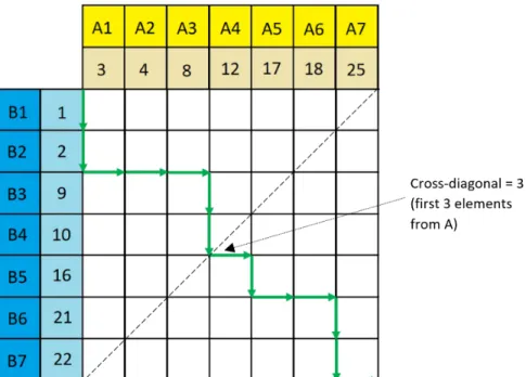
In our algorithm, we have adopted a parallel merge sort algorithm that is using the “merge path” approach [26] to enable merging the sorted chunks in parallel without the need for any communication between threads. At the same time, it ensures a balanced workload for all the threads. The “merge path” approach is a preliminary step before every merge phase so that each thread will know how many elements from each sorted-subarray it can fetch and merge to form a sorted chunk that is part of a larger sorted subarray. The “merge path” algorithm starts by having two sorted subarrays in the form of [A] x [B] matrix, after that, it compares elements from both subarrays to form a merged path that tells the threads in the merge phase the number of elements in each subarray they can fetch and merge. Figure 3.1 illustrates how the series of comparisons can lead to a merged path that can divide the sorted subarrays into independent segments that are called cross-diagonals. In the first phase of

Figure 3.1: An example of the mergePath approach when dividing the merge operation between two threads, the cross-diagonal value determines how many elements each thread can fetch from each subarray. In this example, the first thread will fetch 3 elements from A and 4 elements from B (total = 7), and the second thread will fetch the remaining elements

(4 from A and 3 from B) [25].

the algorithm, the unsorted array will be partitioned into chunks of data, where each chunk will be assigned to a block of threads that will fetch the data chunk into the shared memory to apply the merge-path algorithm on it, and then conduct the merge phase by the threads within each block. As the chunk of data increases in size, the following merge-path and merge phases will require multiple blocks of threads to cooperate in computing these phases. However, because threads within different blocks cannot access other blocks’ shared memory, chunks of data are usually stored in global memory after each merge phase. Similar to the traditional merge-sort algorithm, after a certain number of merge stages, the array will be completely sorted.

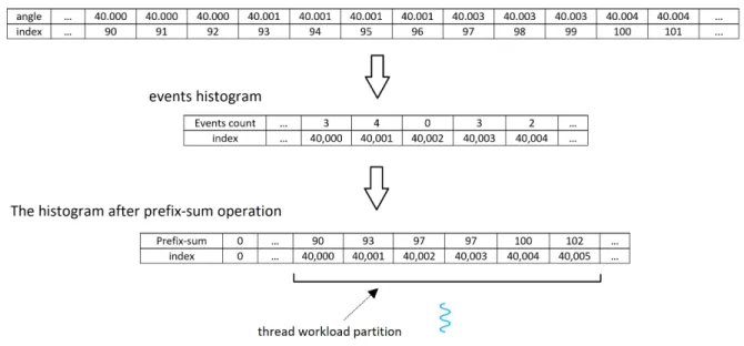
Figure 3.2: An illustration of building a histogram and then applying prefix-sum operation on it so each thread can identify the starting index of its partition in the event-list.

The third step in our algorithm is to build a histogram for the counts of the number of events for each azimuth-angle. For example, the histogram size has been set to 360,000 buckets to contain all events that reside between 0◦ and 360◦ degrees. This step is crucial to know the count of events in every azimuth-angle up to the third digit after the decimal point in the angle’s value. The next step is to apply the prefix-sum operation on the newly built histogram. The output of this operation will enable parallelizing the radial-sweep operation (the final step) where each thread can know at which index in the event-list is the beginning and the end of its sector, as shown in Fig 3.2.

In the last step, all threads will start the radial-sweep operation on their partitions from the event-list (the partition from the event-list form a relatively small sector for a thread to process), where every thread will initiate its status-tree by adding all cells information that would intersect with the sweeping line at the angle that is considered to be the starting point of the designated sector. This can be done by calculating the x-step and y-step of the

starting line based on the angle’s value, where x-step = cos θ, and y-step = sin θ, where

θ is the angle value of the sweeping line where it should start rotating. Then all threads

will start fetching the events from their partitions in the event-list. The main problem here is that the status-tree is a dynamic BST due to its nature in the frequent change of size caused by a large number of insert and remove operations, and implementing a dynamic data structure on the GPU would significantly worsen the algorithm performance, because any memory space in the global memory has to be allocated before any kernel call. However, after carefully studying the nature of the status-tree and the pattern of the event’s operations, we found it is more appropriate for several reasons to use a static BST instead of dynamic as a status-tree. First, it eliminates the cost of frequently rebalancing the tree with every insert and remove operations, which on GPU it means avoiding the continuous re-allocation of the status-tree. Second, the status-tree has a fixed range of the number of cells that will always vary between n/2 and n (if the observation point is in the middle of the elevation-grid, but in a worst-case scenario when the observer is in the corner of the grid the tree size will vary between n and 2n). Thus, it is possible to pre-allocate the space for the status-tree only once based on the maximum possible number of cells that will exist during the line rotation. Also, due to the nature of the events, where any two events that have the same azimuth-angle and distance values, the first one will be a remove event, and the second event is an insert, which will never cause a conflict when adding new cells to the tree (this is why when sorting the event-list, remove events take higher precedence than insert events). The third reason for using a static BST is that all three operations are much cheaper compared to the same operations when being applied to a dynamic BST. Finally, the memory space required for the status-tree is significantly reduced due to the eliminating of pointers that were used to link nodes to each other in the tree, which is always preferable, especially when considering the size of the global memory, which is relatively small. The algorithm is executed using thousands of threads, each one with its own status-tree. The only downfall when using static

BST is that it has to be a perfectly balanced tree. The tree size is calculated based on the maximum possible number of cells the tree will have. If the number of leaf nodes equals n, then the total number of nodes is 2n, and the depth of the tree d is equal (log 2n) + 1.

Thus the total number of nodes in a perfectly balanced BST is equal to 2d _{− 1. However,}

even though the size of the static status-tree is larger, it requires less memory space.

3.2 Optimizing Memory Utilization

In this section, we describe an optimized radial-sweep algorithm which mainly designed to overcome the excessive memory consumption problem, which is the main drawback of the radial-sweep algorithm for computing viewshed and analyzing visibility. The original algorithm [11] and our GPU-based radial-sweep algorithm from the previous section, both generate a significant amount of intermediate results compared to the size of the input and output data, which limits the size of the map that we want to process its visibility. However, our algorithm did significantly reduce the memory space required for the generated intermediate data by using static BST instead of dynamic BST, and also by applying few data compression techniques to reduce memory consumption even further. Our algorithm can process up to 50Kx50K grid size on CPU and 10Kx10K on GPU. Thus, we are proposing a new memory-efficient radial-sweep algorithm on both CPU and GPU to enable us to use less memory and allows for processing larger data.

The event-list is the largest intermediate data generated by the radial-sweep algorithm, which needs a significant memory space. Thus, the new algorithm uses a different approach when processing the grid’s cells to create the event-list.

Instead of processing the whole grid at once to generate the event-list, sorting the list, and then processing the events using the status-tree to compute the visibility, the new algorithm first divides the grid into equal-sized sectors. For each sector, the algorithm will generate its

moving to the next sector. The trick here is to use only one status-tree while processing all consecutive sectors to manage the events that are currently intersecting with the sweeping line, and to keep all data in memory by dividing the elevation-grid into sectors that its event-list can be held in memory, which is a different approach and more effective compared to [13] where they proposed sorting and storing the event-list on disk and then processing it in a streaming manner to resolve the large size of the intermediate data.

3.2.1 The CPU-Based Optimized Algorithm

In this section, we will describe the CPU-based version of the new algorithm. The main challenge here was finding all target cells in a particular sector. In [12], when they tried parallelizing the radial sweep algorithm, and they wanted to find all the cells in a certain sector, they used an approach similar to the R2 algorithm to identify all cells located in a particular sector. Their approach was launching multiple rays from POI to border cells, and with every step, the advancing ray computes the ID of the cell currently crossing. However, their approach can lead to skipping cells if a ray is crossing these cells’ narrow corners, which leads to reducing the overall algorithm accuracy which is one of the reasons why the R2 algorithm is less accurate than R3 and Radial-sweep algorithms.

In our new algorithm, we have adopted a different approach where we first divide the grid into 4 or 8 main regions (quadrants and half-quadrants), as shown in Fig. 3.3. After that, we scan the region(s) where the desired sector is located at. Scanning the associate quadrant(s) or half-quadrant(s) for finding the wanted cells will not add any overhead if the grid is already divided into 4 or 8 sectors. Thus, if a grid is divided into a different number of sectors other than 4 or 8 (e.g., 12, 15, or 30 sectors) (Fig.3.4) it will add additional overhead due to the repeated scanning of a particular region if multiple sectors are located within the same region, or there is a sector that overlapping between different regions which requires scanning all associate regions to find all the cells in that sector See Algorithm-3 for the new

algorithm pseudocode. We have chosen this approach for finding all cell IDs in a target sector because it preserves the algorithm’s accuracy, which is a characteristic we want to maintain in our algorithm. Also, the overhead resulted in scanning regions, even for multiple times is not that significant when having 30 or fewer sectors.

The algorithm first divides the grid into eight main regions (half-quadrants), and for each sector, it searches the associate region(s) where the sector is located at. Also, the same algorithm can be used if we want to divide the grid into 4 main regions (quadrants) instead of 8. When scanning quadrants or half-quadrants, each cell in that region will be processed to generate all three events (insert, inquire, and remove events), and it will only store those events that are within the sector space. Commonly, a cell is partially located within a sector space, and in that case, it will only store the events included in the sector space. Also note that a sector might be located between two scan-regions, which means the algorithm will have to scan these two regions to find all cells within that sector.

3.2.2 The GPU-Based Optimized Algorithm

In order to reduce the impact of the large memory consumption needed for the event-list generated by the radial-sweep algorithm, the same approach has been used in the GPU-based radial-sweep algorithm. We need to divide the grid into multiple sectors, and target cells can be found by scanning the associate quadrant(s) or half-quadrant(s). Due to the very limited memory space available on GPU devices which in our case is around 11 GB, we found that the most practical variation to balance between the algorithm performance and the ability to process the largest possible data is when dividing the grid into 8 sectors and 4 scan-regions, which means scanning the whole target quadrant to find the relative cells. Dividing the grid into less than 8 sectors will result in a significant increase in the event-list size along with a decrease in performance if sectors are overlapping between multiple quadrants. Also, having more than 8 sectors will significantly worsen performance because

Figure 3.3: Dividing the grid into 4 or 8 scan-regions to facilitate searching cell IDs in a target sector.

Figure 3.4: A grid with 8 scan-regions that has been divided into 10 sectors. Some sectors are located over two scan-regions.

of the increasing number of kernels calls from the host side. In the final step (radial-sweep), each thread will have to initiate the status-tree, which can be costly if it kept repeating this step multiple times. Finally, the reason behind scanning whole quadrants instead of half-quadrants as we did in the CPU-based algorithm is because it is difficult to map each thread to its cell in a half-quadrant while it is a straight forward process when mapping threads to the quadrant’s cells.

We have tried multiple approaches to map threads to their cells when scanning half-quadrants. The fastest by far was utilizing a for-loop to find either the cell’s x-value or y-value. Then we can find the other one by finding the first or last thread ID in the target row if we have obtained they-value or the target column if we have obtained x-value from the for-loop above. However, this approach adds non-trivial overhead to the overall performance because when using for-loop on GPU where each group of threads will perform a different number

of iterations. In general, it would cause lots of stalling amongst threads waiting for another group of threads to finish a different set of instructions. Another reason for not adopting this approach is in the preliminary step (where it searches for cell IDs), the memory space needed to maintain the scanning operation is not that significant regardless if it is scanning a whole quadrant or a half-quadrant.

The GPU-based algorithm starts first by allocating memory space on GPU for the elevation-grid array (input data), the event-list, and the visibility-results. All these memory allocations will be reserved during the algorithm life span. Also, as algorithm-4 shows, the event-list size is only a fraction of what it used to be in the non-optimized GPU-based algorithm, while both the input and output data remain the same without any reduction in size. After transferring input data from the host (the CPU) to the device (the GPU), the algorithm will go through all grid’s sectors using a loop, and the host will make seven kernel calls in each iteration. The first two kernels are a preliminary stage that will help each thread in the following stage to know where to store the events information it obtains in the event-list. In the search events kernel, each thread will be mapped to a target cell in the target quadrants, and it will only compute the azimuth angle for all three events of that cell. It will count how many events are included in the target sector, and then it will store the count values in a temporary array. After that, a prefix sum operation on GPU will be applied to the histogram. The reason for that is in the next step when building the event-list for the target sector, each thread will know where to store the generated events by knowing how many events the previous threads will store in the event-list. This was one of the main challenges in designing the new optimized algorithm on GPU because regardless of the size of the sec-tor, each cell will have a different number of events that are within the sector space. Some cells will have less than three events if these cells are partially included in the target sector, and all cells that are located outside the sector region will not have any events to generate and store in the event-list.

The last four kernels are similar to the non-optimized GPU-based radial-sweep algorithm. Still, all of them have been adjusted to work on a smaller event-list generated for a particular sector.

Chapter 4: Evaluation and Results

In this section, we evaluate the performance of our parallel GPU-based radial-sweep algo-rithm [25] and compare it with the GPU-based R3 and their original sequential algoalgo-rithms on CPU. Also, we show the effectiveness of using a static BST in the status-tree instead of dynamic BST in the original radial- sweep algorithm on CPU. Finally, we will show the performance evaluation of our new optimized CPU-based and GPU-based algorithms. In all experiments, we have used the NVidia Titan V graphic card to execute all the GPU-based algorithms. The GPU is GPU-based on NVidia Volta architecture, and it consists of 5120 computing cores distributed equally between 80 streaming multiprocessors along with 11 GB global memory. For the CPU-based algorithms, we have used AMD Ryzen Thread ripper 1950x 16-core 2.15 GHz processor on a machine running Ubuntu 18.04.3 LTS operating sys-tem, and we used NVCC10 for compiling all CPU and GPU code.

The data used in the experiments are STRM datasets that had been used in [12], and the datasets come in different sizes starting from (5000 x 5000) up to (30,000 x 30,000) cells. Also, in the first experiment, we have used an additional DEM file that represents the topol-ogy of Germany that can be found in [27].

Finally, in the last section of this chapter, we show some of the optimization techniques that have been applied to the original parallel merge-sort on the GPU.

4.1 Parallel GPU-based radial-sweep Algorithm

In this section, we have conducted two experiments using different datasets to measure the performance of our first parallel GPU-based algorithm (described in section 3.1 ), and we compared it with three other algorithms: sequential R3, sequential radial-sweep, and GPU-based R3. In general, all experiments show the superiority of the GPU-GPU-based algorithms over the CPU-based algorithms is at least two orders of magnitude.

In the first experiment, we have used an elevation-grid of size (10800 x 10800) obtained from [27]. The data is an SRTM Digital Terrain Model of Germany where elevations are measured using ”meters”. Some of the measure aspects of the map are presented in table 4.1.

Table 4.1: Description for the data used in Section 4.1, and obtained from [27].

Data descriptor Measurement (meter)

Maximum elevation value 1592

Minimum elevation value 0

Average elevation value 12

Percentage of cells with elevation value equal to 0 21.64%

Figure 4.1 shows that our algorithm has significantly better performance than all the other three algorithms. Our GPU-based radial-sweep is 3.5x faster than its fastest competitor the GPU-based R3. Also, it is faster than its sequential version by around 2000x, and around 6200x compared to the sequential R3 algorithm.

In the second experiment we have used two elevation-grids provided by [12], where their sizes are (5000 x 5000) and (10,000 x 10,000). Similar to the previous experiment, our GPU-based radial-sweep algorithm maintained the same speedup compared to the GPU-GPU-based R3 when processing the larger elevation-grid that is similar in size to the one we used in the previous experiment. However, when using a smaller size data, the difference in performance between the two GPU-based algorithms is reduced. When the data size is (5000 x 5000),

Figure 4.1: Comparing all already known exact-viewshed algorithms with our GPU-based parallel radial-sweep algorithm using a grid size of (10800 x 10800).

our GPU-based radial-sweep algorithm is 2x faster than the GPU-based R3 (Fig. 4.2). This experiment also shows that our algorithm gains more speedup over R3 on GPU when processing larger data.

Fig. 4.3 illustrates the time break down for our parallel radial-sweep algorithm on GPU. 62% of the execution time goes to the radial-sweep phase, which is the final step in the algo-rithm and the most time-consuming phase. The second time-consuming step is the sorting step, which makes 23% of the total execution time. Building the histogram step makes 7% of total execution time. Note, however, there is a possibility for further optimization here if shared memory would be used to improve the performance of this operation, but optimizing histogram operation will have negligible improvement compared to the overall performance. The shortest steps in our algorithm are applying prefix-sum on the histogram and event-list building step which is the very first step in the algorithm. The cost of performing prefix-sum on the histogram was minimal (2.5 milliseconds) which is around 0.15%, and building the

Figure 4.2: Comparing all exact-viewshed algorithms using different datasets.

event-list is 1.5% of overall execution time. Finally, the time required for transferring data to and from the GPU device composes a little over 5% of the total execution time. In other words, 5% of the algorithm execution time is for I/O, while 95% is the actual implementa-tion. See Fig. 4.4,

4.2 The efficiency of using static BST

To measure the efficiency of using static BST in the radial-sweep algorithm instead of the conventional dynamic BST as the status-tree that manages the events generated by the algorithm, we have designed a new sequential CPU-based algorithm similar to the original radial-sweep, where the new algorithm uses a static BST as the structural base for the status-tree. In the experiment, we tested both algorithms on datasets that vary in size. Figure

Figure 4.3: The break-down of execution time for GPU-based radial-sweep algorithm stages taken from the first experiment

Figure 4.4: The break-down percentage of the I/O portion and the computation portion of the overall execution for parallel radial-sweep on GPU

Figure 4.5: Showing the efficiency of using a static BST in building the status-tree instead of the conventional status-tree built using a dynamic BST over different data sizes. The

new approach improved performance by up to 44x.

algorithm performance by up to 44x.

Also, as we mentioned earlier, the new status-tree requires less memory than the conventional approach. Figure 4.6 shows our unique approach can reduce memory space needs the status-tree by up to 70% to 80%, which is significant, especially when processing large data.

4.3 Memory-optimized radial-sweep algorithm

In this section, we evaluate both our new optimized algorithms. For the optimized CPU-based algorithm, we have compared it against the sequential static BST-based

algo-Figure 4.6: Comparing memory requirement for the status-tree for two CPU-based sequential radial-sweep. The first algorithm used the conventional dynamic BST, and the second used the new static BST. The experiment shows the new status-tree requires 70%

wherein each case we have set a different number of sectors. Also, we want to show the opti-mal number of sectors that work best with the new optimized algorithm. We have designed two variations of the new algorithm, where the first variation scans a whole quadrant to find cell IDs in a target sector, and the second variation scans a half-quadrant instead.

In Figure 4.7, we compared both variations of the new algorithm using a grid of size (25,000 x 25,000), along with their different cases. The experiment shows that dividing the elevation-grid into sectors and processing each one of them separately does not add any computation overhead in both variations when the number of sectors is 16 and less. In fact, in some cases, when the grid is divided into 12 sectors or less, the new algorithm is slightly faster, and it can achieve up to 6% performance gain compared to our previous sequential static BST-based algorithm. This is because sorting s partitions of the event-list are faster than sorting the whole list. Another reason for the performance boost is that when dividing the grid into 4 or 8 scan-regions, the search operation for a target cell’s ID requires less number of if-statements (which is needed to verify which of the eight regions a cell is located at). However, as the number of sectors goes up, half-quadrant variation shows a significantly better performance than the full-quadrant variation.

To show the reduction in memory consumption of our new algorithm compared to the previous one, we will show the memory space required for the algorithm before and after using segmentation. In the first example, when processing a grid of size 25000x25000: Input size = 2.32 GB

Status-tree = 0.5 MB (very negligible)

Event-list (without segmentation) = 38.42 GB Event-list (with 30 sectors segmentation) = 2.32 GB

The second example will show needed memory when computing viewshed for a grid of size 100Kx100K:

Input size = 37.25 GB

Event-list (without segmentation) = 614.7 GB Event-list (with 30 sectors segmentation) = 20.5 GB

Finally, for the new optimized GPU-based algorithm, we compared it with our pre-vious parallel GPU-based radial-sweep algorithm and with the GPU-based R3 using five elevation-grids in different sizes. Figure 4.8 shows when the grid size is small, the difference in performance between all three algorithms is very subtle. However, as the data size in-creases, the difference is more obvious. In all cases, the R3 algorithm needed much more time than the other algorithms. For the non-optimized parallel radial-sweep, it can only process data up to the size of (10K x 10K) due to the large intermediate results that require more memory space than the current GPU’s global memory can offer. In the first two cases, the new optimized algorithm is two times slower than the non-optimized one, but as the data size increases, the difference in performance between the two is decreasing. There are two reasons for the decrease in performance of the new optimized algorithm: the segmentation process (the additional two kernel-calls for cell-search operation ), and having all kernels in a loop to process sectors sequentially adds significant overhead to the overall execution time. However, despite the decrease in performance, the GPU-based radial-sweep algorithm can compute visibility for larger data. In the last three cases, we compare the optimized radial-sweep with the GPU-based R3 algorithm, and as the experiment chart shows, our new algorithm has achieved up to 4.4x times speedup over the R3 algorithm. In terms of input size, the optimized algorithm can process up to 6.25x more data than our previous non-optimized algorithm.

Figure 4.7: The execution time of two variations of the new optimized CPU-based radial-sweep algorithm when dividing the data into a different number of sectors using a

data size of (25K x 25K). The first variation search for cell IDs in a target sector by scanning a “full quadrant”. While the second variation searches for cell IDs by scanning a “half quadrant”. The experiment shows both variations maintain the same performance as the original algorithm when dividing the grid into 12 or fewer sectors. Also, the algorithm

based on the “half quadrant” search-region shows significantly better performance when dividing the data into a large number of sectors. The “original” case refers to our

Figure 4.8: Measuring the performance of all three exact-viewshed algorithms over data in different sizes. The original GPU-based radial-sweep algorithm cannot process data larger

than (10K x 10K).

4.4 Optimizing the Merge-sort (MergePath) Algorithm

Before we show the proposed optimizations for the sorting algorithm, we first will ex-plain the original algorithm presented in [26]. The algorithm is composed of 3 essential steps shown in Algorithm-5. In the first step which called “KernelBlocksort”, the unsorted list will be divided into several chunks of data each of the size NV (Number of Values) where the NV = 2816 elements. Then each chunk will be sorted within a block of threads.

The second and third steps will constantly be called in a loop until the list is sorted. Similar to a typical merge-sort algorithm, the number of iterations is equal to (log n) + 1

where n is the number of elements in the list. The second step “MergePathPartitions” goal is to compute the “global partition parameters” which are the values that determine how the new partitions of data are distributed equally amongst the blocks. After that, in the

Figure 4.9: Algorithm-5 A high-level abstraction of the MergePath algorithm on GPU.

third step, each block of threads will compute the cross-diagonal value (Fig. 3.1) on its designated partition, and then each thread will fetch a certain number of elements from two sorted sublists based on the cross-diagonal value.

In order to improve the performance of the merge-sort (MergePath) algorithm on GPU, two attempts have been conducted and explained in detail along with the experimental re-sults that compare the execution time for the original algorithm vs the optimized algorithm. First, in Step1 and step3 the VT (values per thread) has been increased for each thread to reduce the overall amount of computation with the cost of using more shared memory which did not give any enhancements. Second, in Step2 each thread will compute multiple MergePaths for multiple chunks which showed an acceptable increase in performance com-pared to the original algorithm. Note that we have been working on mergeSortPairs() where

it sorts a list based on keys and their relative values to its new relative position in the sorted list.

As it has been mentioned, increasing the value of VT will reduce the amount computation by reducing the overall number of calling “MergePath” function (where parameter p is cal-culated based on a series of comparisons on two sorted chunks). So, for 100 Million elements when VT=11 the number of calls for “MergePath” will be a little over 9 million times, and this only for a single iteration in step1. When VT=22 the number of calls will be cut to half, but with the cost of using more registers than already available to a single thread which creates the need for using shared memory to store and load the extra values. The afore-mentioned modification effects both steps 1 and 3. Step2 uses different settings and these changes won’t affect it. In table-1 we can see that the general performance is worsened by a small fraction of time in most cases due to the use of shared memory to store more values when there are not enough registers for each thread which counters all benefits gain from reducing the overall amount of computation. Thus, there is no benefit from increasing the value of VT per thread, and it shows that the optimal VT value is 11.

Table 4.2: Performance results for original implementation (VT=11, NT=256) vs. new implementation (VT=22, NT=128) on a list of size 100M elements (time in millisecond).

VT = 11, NT = 256 VT = 22, NT = 128 Overall evaluation 477.5 518 Worst 514.3 428.3 Better 470.9 505.2 Worst 516.4 487.4 Better 419.9 426.1 Worst 422.9 430.1 Worst 516.4 525.2 Worst 418.4 425.4 Worst 421.3 430.6 Worst

The second attempt for optimizing the MergePath algorithm is by redistributing the workload for each thread in step2. Each thread will do the work of two threads in the orig-inal algorithm by calculating two consecutive “global partition parameters” instead of one. In theory, the benefit of such modification is that the total number of threads will be reduced by half, and we only need to calculate MergePath initial parameters such as frame, a0, b0, and b1 only once for every two chunks, because these parameters are the same for a group of threads working on a certain coop number (e.g. for coop=4 threads 0, 1, 2, and 3 will have the same initial parameters when calculating MergePath). The only parameter that makes a difference when calculating MergePath is the thread number in a group of coops). See figure 4.10 for illustration on how the new approach works for coop=2 and coop=4.

To further improve performance, each thread will aggressively compute all MergePaths’ cross-diagonal values for all the chunks in a coop. See figure 4.11. Besides the benefits we gained from the previous optimization, now there is a higher chance of reducing divergence among threads where threads are will execute the same instructions more often (especially within a warp). This is because the overall number of comparisons is almost the same, wherein the original algorithm the number of comparisons varies between threads based on the thread position in a coop of threads (first thread in a coop of threads will do the least number of comparisons where the last thread will do the most number of comparisons). This modification will raise the question: Will we continue to aggressively compute all MergePaths for a coop until the end of the execution? Well, the answer is no. For a list of size 100M elements and the size of a chunk is 2816 element, the coop will start from 2, 4, 8, 16, . . . ., to 65536 (in total we have 35512 chunks and 216 = 65536). So in the last iteration, only one thread will be running to compute the MergePath for all 35512 chunks so it is obvious that we should not let the new approach be executed to the end.

Figure 4.10: Illustration on how to combine the workload of two threads to be executed by only one thread.

Figure 4.11: Combining the workload of multiple threads to be executed by only one thread.

executing and go back to the original implementation for Step2. Using current available GPUs and with a list size of 100M, the optimized approach should run until coop = 512, after that we should go back to the original implementation. If we kept running the new approach further, the performance will start degrading when coop = 1024 or more.

The experiment has been conducted using GeForce GTX Titan X graphic card, and it has been conducted multiple times due for using randomly generated data which could give a varying execution time for both approaches. In general, our approach outperforms the original algorithm in 74% of the cases when working on uniformly distributed data. On average, our algorithm reduces the overall execution time for MergePath by around 8%, and it can go up to 17% on multiple occasions (Fig. 4.12).

Figure 4.12: The execution time of the original and the optimized MergePath algorithm. The optimized version shows 8% speedup.