Performance assessment of Surrogate model integrated with sensitivity analysis in multi-objective optimization

(1)

Dipartimento di Ingegneria Civile, Edile Ambientale

Department of Civil, Environmental and Architectural Engineering

Corso di Laurea Magistrale in Ingegneria Matematica

Performance assessment of Surrogate

model integrated with sensitivity

analysis in multi-objective optimization

Relatore:

Chiar.mo Prof. Ernesto Benini

Laureando:

Federico Genovese

Matricola:

1129918

(2)

(3)

(4)

(5)

This Thesis develops a new multi-objective heuristic algorithm. The optimum searching task is performed by a standard genetic algorithm, the Non-dominated Sorting Algo-rithm II (NSGA-II). Furthermore, it is assisted by the Response Surface Methodology surrogate model and by two sensitivity analysis methods: the Variance-based, also known as Sobol’ analysis, and the Elementary Effects. Once built the entire method, it is compared on several multi-objective problems with some other algorithms, also these based on evolutionary searching process and on surrogate models. Finally fitting qualities of Response Surface method is tested on an experimental dataset, to measure its predicting features on external data. The final results show that this new meta-heuristic performs well compared to other algorithms and it also seems to be cheap, talking about the computational costs.

This work deals in the first chapters with theoretical aspects, then it introduces the developed model and finally it reports the results of tests on multi-objective problems and of the fitting over the external dataset.

Chapter 2 introduces the mathematical description of a multi-objective optimiza-tion problem. Then it describes the concepts of Pareto optimality, which involves the dominance between solutions and the set of best elements. Successively it deals with the main problems arising working in this framework: the curse of dimensionality and the No free lunch theorem. Last, the chapter introduces the metrics to evaluate the performances of the optimization algorithms.

Chapter 3 describes the main features of the evolutionary algorithms and their typical frame. Then the chapter goes more in detail through the structures of the most spread algorithms. Here the features and the building blocks of each routine are explained to highlight the positive aspects and the drawbacks of each model. In the end of the chapter some non-evolutionary algorithms are introduced. However, these are widely used or much near to the evolutionary ones.

In chapter 4 the typical frames of surrogate model are described and few of them are reported in detail. These are the Artificial Neural Network, the Kriging filter and the Response Surface Method, which it is adopted in the developed model. Finally, there is a brief section which treats the classification of meta-heuristic hybrid optimization methods.

Chapter 5 regards the sensitivity analysis in all its features. First, it reports the main sampling methods with their pros and cons. Successively the most used sensitivity analysis methods are described, dealing also with the mathematical concepts.

In chapter 6 the building of the developed methods it is explained in details. First of all, it introduces the general results of sensitivity analysis for the test problems at hand. Then it treats in each feature the Response Surface Methodology and another point worth highlighting is the new parameter differing from the literature suggestion.

(6)

Finally, it is described also the genetic algorithm used to perform the optimization searching process.

Chapter 7 deals with the results of the optimization task, both for two- and three-objectives test functions. However, before it reports the results, there are introduced the algorithms which allow the comparison. Then just two problems are reported, one from two-objectives test and one from the three-objectives. The complete definition of test functions can be found in appendix A, while the complete results in appendix B.

Finally, chapter 8 analyses the behaviour of the Response Surface on the external dataset. First, it describes the nature of the dataset and its application. Succes-sively, the chapter introduces the methods with which will be evaluated the goodness of predicted data from the Response Surface. Therefore, few results are reported and commented for each method. Again, the complete results can be found in appendix, in chapter C.

(7)

This work comes up from the knowledges acquired during my entire academic studies, but also due to the curiosity and the appeal that this topic inspired me.

A huge thank goes to all those who make this goal possible, sustaining me during all these years: my parents and my family, all my friends and the class mates, with which I shared disappointments and satisfaction and all the people who have been next to me.

Particular thanks go to Prof. Benini for his valuable suggestions and his kindness. I would also like to extend my thanks to Dott. Venturelli, who shares useful his knowledge, several information and data.

Finally, I wish to thanks all those people who help me with their suggestion to build up, review and correct this work.

(8)

(9)

Abstract v

Acknowledgements vii

1 Introduction 1

1.1 Objective of the Thesis . . . 1

1.2 Summary of the Thesis . . . 1

2 Multi-objective optimization 3 2.1 Mathematical description . . . 4

2.1.1 Pareto optimality . . . 5

2.1.2 Curse of dimensionality . . . 7

2.1.3 No free-lunch theorem . . . 8

2.2 Algorithm evaluation metrics . . . 9

3 Evolutionary Algorithms 13 3.1 Evolutionary Algorithms . . . 13

3.1.1 Main features . . . 13

3.2 Genetics algorithm . . . 15

3.3 Particle swarm optimization . . . 20

3.4 Differential evolution . . . 22

3.5 Shuffled frog leaping . . . 25

3.6 Ant colony optimization . . . 27

3.7 Other meta-heuristic methods . . . 28

4 Surrogate Models 33 4.1 Main features . . . 33

4.2 Kriging . . . 36

4.3 Artificial Neural Networks . . . 41

4.4 Response Surface Methodology . . . 44

4.4.1 Local reference frame and sampling . . . 47

4.4.2 Surface fitting . . . 48

4.5 Meta-heuristic hybrid optimization . . . 49

5 Sensitivity Analysis 55 5.1 Purpose of the sensitivity analysis . . . 55

5.2 Sampling technique . . . 56

5.2.1 Random sampling . . . 56 ix

(10)

x

5.2.2 Factorial sampling . . . 57

5.2.3 Latin hypercube sampling . . . 58

5.2.4 Multivariate stratified sampling . . . 59

5.2.5 Quasi-random sampling . . . 60

5.3 Sensitivity analysis methods . . . 64

5.3.1 One at a time . . . 64

5.3.2 Elementary Effects . . . 65

5.3.3 Variance-based method . . . 67

5.3.4 Derivative-based method . . . 70

6 Model Implementation and Application 73 6.1 Sensitivity analysis application . . . 73

6.1.1 Sobol’ sensitivity analysis . . . 74

6.1.2 Morris sensitivity analysis . . . 77

6.2 Response Surface modelling . . . 81

6.3 Genetic algorithm application . . . 85

7 Result and comparison on Test Function 87 7.1 Sensitivity analysis results . . . 87

7.2 Response Surface configuration . . . 88

7.3 Final results . . . 90

7.3.1 Analysis of two-objective test functions . . . 91

7.3.2 Analysis of three-objective test functions . . . 94

8 Analysis of the Response Surface on an experimental dataset 97 8.1 Fitting and testing sets . . . 98

8.2 One point excluded test . . . 100

8.2.1 Global response surface result . . . 101

8.2.2 Local response surface result . . . 101

8.3 Brief conclusions on response surface methods . . . 102

9 Conclusions 105 A Test Functions 107 A.1 Two-objectives test functions . . . 107

A.2 Three-objective test functions . . . 109

B Plots and Data of Test Functions 113 B.1 Results of two-objective problems . . . 113

B.2 Results of three-objective problems . . . 120

C Box-plots of errors on the experimental dataset 129 C.1 Fitting and testing sets box-plots . . . 129

C.2 One point excluded global tests box-plots . . . 132

C.3 One point excluded local tests box-plots . . . 135

(11)

2.1 Pareto Front . . . 6

2.2 MOOP evaluation metrics . . . 9

3.1 Crossover techniques . . . 18

4.1 Parameters θ and p . . . 38

4.2 ANN classification . . . 42

4.3 Sigmoid and Hyperbolic tangent functions . . . 43

4.4 Response surface example . . . 46

4.5 Flow diagram of a Meta-heuristic hybrid optimization . . . 51

4.6 Meta-heuristic calssification . . . 53

5.1 Factorial design . . . 57

5.2 Multivariate stratified sampling . . . 60

5.3 Discrepancy . . . 61

5.4 Sample size of quasi-random sequences . . . 61

6.1 Histogram of Sobol’ sensitivity analysis . . . 75

6.2 Variation on sample dimension for Sobol’ analysis . . . 75

6.3 Histogram of second order Sobol’ sensitivity analysis . . . 76

6.4 Histogram of Elementary Effects analysis . . . 78

6.5 Histogram of Elementary Effects analysis by groups . . . 79

6.6 Variation on sample dimension for Morris analysis . . . 80

6.7 Variation of secondary factors fixed parameter on 2d problem . . . 83

6.8 Variation of secondary factors fixed parameter on 3d problem . . . 84

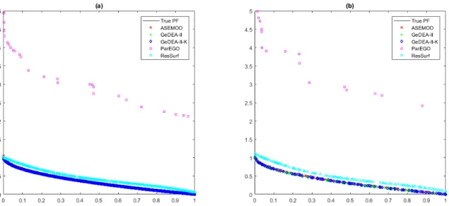
7.1 ZDT1 Pareto fronts . . . 92

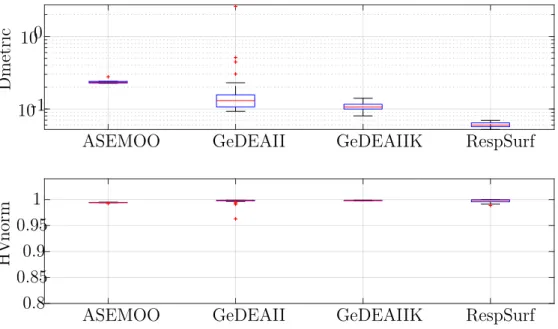
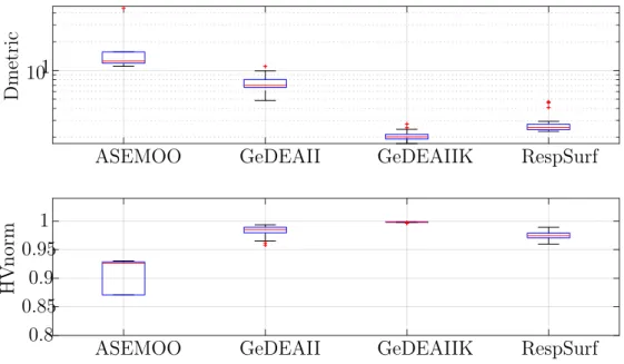
7.2 ZDT1 box-plot of Dmetric and HVnorm . . . 92

7.3 DTLZ2 Pareto fronts . . . 94

7.4 DTLZ2 box-plot of Dmetric and HVnorm . . . 95

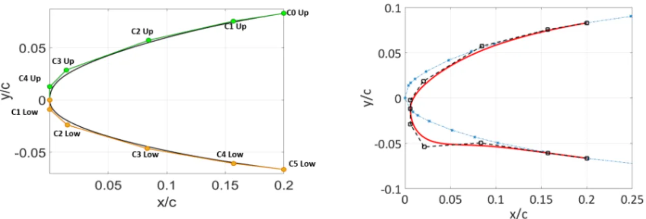
8.1 Airfoil profile . . . 97

8.2 Morphing part of airfoil profile . . . 98

8.3 Error on fit&test method response surface of 5 variables . . . 99

8.4 Error on fit&test method response surface of 6 variables . . . 99

8.5 Mean error Vs number of variables on fit&test method . . . 100

8.6 Global response surface of 6 variables . . . 101

8.7 Mean error Vs number of variables in global surfaces . . . 102

8.8 Local response surface of 6 variables . . . 102

8.9 Mean error Vs number of variables in local surfaces . . . 103 xi

(12)

B.1 ZDT2 Pareto fronts . . . 113

B.2 ZDT2 box-plot of Dmetric and HVnorm . . . 114

B.9 DTLZ1 Pareto fronts . . . 120

B.10 DTLZ1 zoom on the Pareto front . . . 120

B.11 DTLZ1 box-plot of Dmetric and HVnorm . . . 121

C.1 Error on fit&test method response surface of 1 variable . . . 129

C.2 Error on fit&test method response surface of 2 variables . . . 130

C.5 Global response surface of 1 variable . . . 132

C.6 Global response surface of 2 variables . . . 132

C.10 Local response surface of 1 variable . . . 135

C.11 Local response surface of 2 variables . . . 135

(13)

4.1 Axis sample . . . 48

4.2 X matrix construction . . . 49

5.1 Fractional design . . . 58

5.2 Doubled Latin Hypercube sampling . . . 59

5.3 Halton sequence . . . 63

5.4 Sobol sequence . . . 64

6.1 Sobol’ analysis results . . . 74

6.2 Sobol’ second-order analysis result . . . 76

6.3 Morris sensitivity analysis . . . 77

6.4 Morris sensitivity analysis by group . . . 78

6.5 Number of generation . . . 86

7.1 Sensitivity analysis of ZDT3 and DTLZ2 . . . 88

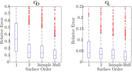
7.2 Surface errors variability on two-objective problems . . . 89

7.3 Surface errors variability on three-objective problems . . . 89

7.4 ZDT1 data of Dmetric and HVnorm . . . 93

7.5 DTLZ2 data of Dmetric and HVnorm . . . 95

B.1 ZDT2 data of Dmetric and HVnorm . . . 114

B.5 DTLZ1 data of Dmetric and HVnorm . . . 121

(14)

Chapter 1 Introduction

1.1 Objective of the Thesis

This work aims to develop a new meta-heuristic evolutionary optimization tool building together a surrogate model with sensitivity analysis. While the surrogate is a tool quite diffused in the optimization frameworks, sensitivity analysis is often accounted as a mere statistical one. The coupling of these two implementations can lead to effective information and results.

Besides, they could provide some sort of simplification to the optimization at hand. Building this optimization tool, a further aspect to deal with is the computational cost. Nowadays many high-fidelity models reach astonishing results, e.g. they manage to reproduce with computer-based experiments almost exactly the features of real-based ones, while they also retrieve larger quantity of data than the real experiments. On the other hand, these high-fidelity models require huge amount of computational resources and time, which limit often their filed of application. Here the model to be developed will be a cheap one. It should be able to decrease the computational requirements with respect to many other algorithms, while returning a controlled level of accuracy.

Moreover, optimization methods work on an entire process, developing it in all its features. Anyway, external data could be submitted to the model to perform the optimization. Often, in this case external data do not present the desired sample required by the model itself. In fact, most of the times the sampling phase of an optimization problem is realized through the Design of Experiments [10, 48]. The latter provides the most useful information possible to the model, so that it will show better performance. Here the aim is to build a model able to fit also external data.

Thus, the main focus of this thesis is to set up a cheap meta-heuristic model. To realize such algorithm, both a theoretical analysis of each aspect connected to the meta-heuristic model and a detailed implementation of the part involved are necessary. In particular, many parameters can be set in the coding of the response surface model. Despite it is often accounted for as a method not that much suitable, it can prove to be a useful and effective tool, as will be shown in the following.

1.2 Summary of the Thesis

To achieve the above objective, the initial feature of this work is a theoretical analysis of all the involved parts, which are a multi-objective optimization, an evolutionary

(15)

search algorithms, surrogate models and sensitivity analysis. The development of each argument through the text follows the sequence in which they had been encountered and studied from the literature.

Once done this, the effective model construction is described. The first step consists in the coupling of sensitivity analysis with the surrogate model. Between those that have been red and reported in the bibliography, few articles use and take advantage of this statistical test to provide further information upon which they base the surrogate. A profitable tool which can give large amount of information without requiring too much computational efforts can be obtained. The sensitivity analysis not only describes to the user which are the main variables influencing the function. It also provides much useful general data about the behaviour of the problem.

The successive phase to build the meta-heuristic deals with the research of a sur-rogate model able to retrieve good solutions but at the same time it results cheap, computationally speaking. To this scope, some algorithms have been studied and the most suitable was identified in the response surface. This last shows a large simplifica-tion to the problems, so it allows to perform the choice of the evolusimplifica-tionary algorithm once again looking to the computational complexity. Finally, the resulting model is evaluated on the test problems to measure its features and its abilities to perform the optimization task for which it has been built. Although test problems cannot measure completely the qualities of the model, they are necessary to realize further tests. In particular, it is important to evaluate the method’s ability to fit experimental sample of data coming from a general set up and not based on the required sample set.

At the end of the thesis the results for all these tests are reported, evaluating the overall performance which the model shows. It is also sided to other evolutionary algorithms to compare their results on the considered problems.

(16)

Chapter 2 Multi-objective optimization

In engineering Optimization is the process which through an algorithm aims at iden-tifying the combination of variables realizing the best solutions in the problem case at hand. Multi-objective optimization encloses all the problems handling two or more objectives which need to be contemporaneously satisfied. In fact, it can be found variables configurations obtaining good performance only in a single-level or within few-objectives-level. Thus, multi-objective optimization deals not only with the best solutions searching phase, but also with their classification and sorting. The entire process needs to analyse the behaviour of all the variables in their domain to build a profitable and complete optimum search.

Since optimization task needs to interface with complex and various real applica-tions, it faces several problems. The first problem at all is the definition of the objective functions themselves: the mathematical formulation of the case at hand is the intro-ductory step to start with. Without it, it is impossible to begin an analytic search of optima. Mathematical formulation requires first the definitions of variables and their domain. Following this, it is fundamental to identify the proper laws describing the process and the true objectives to optimize. Constrains of each variable also play a main role in the framework. This mathematical translation often is not that easy to set up, because experimental qualitative manner must be reported in a quantitative setting and therefore they become difficult to handle. This sets several errors in the model, which need to be highlighted and possibly solved by running repeated tests before applying the model into practise.

Once the problem is analytically defined, the optimum search sets in. In a multi-objective frame, seldom it is found a sole optimum configuration, dominating all the other framework. Objectives are often mutually competitive and if a solution achieves better values in an objective, it also loses ground on the other sides. Computationally speaking, multi-objective problems require larger quantity of resources (e.g. time and memory) as larger is the number of variables or objectives, the precision required or the sparsity of optima solutions in the domain.

The algorithm chosen to perform the optimum search in this work will be presented later in chapter 3. It is important to highlight since now that several search routines exist, each one with its own peculiarity. Moreover, they often are sided by surrogate models which aim to ease the computational cost. In this optimization framework one can find also many other analytical searching tools, known as Gradient searching meth-ods, as the Conjugate Gradient, the Steepest Descent, and many others. Though, they are seldom used in real-world engineering, where objective functions are too general,

(17)

presenting many local optima. Such methods often get stuck in these local optima, preventing the optimization task to come to a proper end.

Finally, dealing with multi-objective problems it is also necessary to define metrics to classify and to order the proposed solutions, but also the differences between algo-rithms. In fact, once realized which one is the right algorithm, one needs also to know which are its performance with respect to other proposed routines.

This chapter will introduce and describe in detail the mathematical aspects of multi-objective optimization. It will also treat some of the problems hinted here.

2.1 Mathematical description

Single objective optimization aims to find values for the n decision variables x = (x1, x2, . . . , xn) in the domain of decisionΩ, to minimize the objective function:

y= min

x∈Ωf(x) (2.1)

Often in this problem the goal is not only to discover the optimum value attained by the objective (possibly global optimum and not local). The goal is also to find out the set of decision variables which achieve the optimum value. This because the op-timization process is related to a real-life problem and the variables describe a real configuration of the case study. Problems usually are defined as minimization by con-vention, but nothing changes when dealing with maximisation, since the problems are equal: maxf(x) = min(−f(x)). However, searching for the minimum will help to treat multiple objective functions.

The decision variables affect the optimization task with their number, their domain of admissible values and the possible mutual dependencies. Although often decision variables are considered mutually independent and realize a huge relaxation on prob-lems, in almost any application they are continuous in the domain and the objective functions are multi-dimensional. Summing up these features, the single objective opti-mization can reach a high level of complexity by its own. Therefore, efforts are required to formulate exactly the problem and retrieve the optimum solutions.

Beside the objective functions, commonly the problem is affected by constraint expressions. These can be linear or non-linear equations, as well as inequalities, and they could also involve mixed-integer problem (MIP). In mixed-integer problems some decision variables are integers within their domain. This kind of optimization requires specific solvers [48]. For example, a generic problem like this can be written as:

Solve: y= min

x∈Ωf(x)

Subject to: gi(x)≤0, i= 1, . . . , k

xj ∈Z, j ∈1, . . . , n

Constrains involving integer variables make the optimization much more difficult, since it becomes a kind of discrete problem. Anyway, the presence of constrains, their de-velopment and evaluation increase the complexity, affecting the optimization process.

(18)

5 2.1. Mathematical description

Dealing with multi-objective optimization, only the number of objective functions changes tom (withm ≥2). The new problem can be written by defining a new function

F(x) = (f1(x), f2(x), . . . , fm(x)), which maps the vector xof the decision variables of

dimension N to the vector yof the objective functions space with dimension m:

y= min

x∈ΩF(x) (2.2)

Such optimization requires to evaluate simultaneously all the objectives. This implies increasing complexity and computational cost. Moreover, these objectives represent several features of a problem, often bringing opposite contributes to each other. So, as will be analysed in details in the following sections, getting a better value on some objectives often means worsening some others. As the number of objective functions increases, the problem becomes more complex and typically 10 objectives are set as threshold from an easy problem to a harder one. One of the major challenge of multi-objective optimization is to deal with computationally expensive multi-objective functions. Such problem shows up often in simulation based models (e.g. FEM, CFD), which require huge resources to solve even quite simple problems.

2.1.1 Pareto optimality

Mathematical optimization focus on determining the global best solution for a given problem. Often this is not possible in practice, for several reasons: first of all, opti-mization works with a model of the real problem. Therefore, the solution obtained will be affected by errors due to the fact that equations can’t perfectly describe reality. Second, dealing with complex function in many variables, the function value attained at its optimum and the optimum point itself is unknown. So, it is not even possible to understand if it is close to points already evaluated. Finally, it can be proven with test functions that reach the global optimum it is very time consuming when the num-ber of variables is large (typically fairly difficult optimization problems has at least 30 decision variables).

Searching for the best solution of a function, it is possible to identify also two other optimum regions: the local one and the robust one. The former represents usually a problem because the searching process need to overcome this region and proceed to the global optimum. The robust region displays a wide area where, changing the variables, function attains more or less the same value. This could allow to develop more carefully the analytical model, inserting new variables and searching in this area for an optimum in the new formulation.

When some functions achieve multiple good solutions, they get called multi-modal. In these cases, multiple optima provide to the designer a choice, but this multiplicity always depends on the model developed. On the other hand, dealing with a multi-objective problem, when the optimization finds out several good solutions, each of them taking the best value on a different function, these are called Pareto solutions.

The following definition are the fundamental concepts in multi-objective optimiza-tion, as stated in [61]:

Pareto Dominance Given two vectorsu= (v1, v2, . . . , vm)and v= (u1, u2, . . . , um), u is said to dominatevand denoted asu≺vif and only if∀i∈ {1, . . . , m}, ui ≤

vi∧ ∃j ∈ {1, . . . , m}:uj < vj. Moreover,u is said to cover v, denoted as uv,

(19)

Pareto Optimality A solution x ∈ N is said to be Pareto optimal with respect to the whole set N if and only if there is no other solution x0 ∈ N for which

F(x0)≺F(x).

Pareto Optimal Set For a given multi-objective evaluation function F : N → M

the Pareto Optimal Set is defined as the subset of N of all the Pareto optimal vectors in the decision variable set:

P areto Optimal Set=. {x∈N:_@x0 ∈N:F(x0)≺F(x)}

Pareto Front For a given multi-objective evaluation function F : N → M and a

Pareto Optimal Set, the Pareto Front is defined as the set of vectors mapped from the Pareto Optimal Set to M by the objective function F:

P areto F ront=. {y=F(x) = (f1(x), . . . , fm(x)) :x∈P areto Optimal Set}

Many real-world problems involve conflicting objectives which need to be solved together. This framework requires the use of the above concepts to rank and evaluate which are the best solutions. A generic example is reported in figure 2.1, that presents a problem concerning minimization of costs and time delays in a transmission system. As obvious, increasing the velocity of data broadcasting requires better infrastructures, though also higher costs and vice versa, lower investments involve worse performance. The points A, . . . , F on the graph represent the possible solutions individuated, but only the pointsA, . . . , E are reasonable solution. This happens becauseF would realize higher delays with the same cost of A, while G higher cost with the same delay of D. Hence solutions F and G are the so called dominated solutions, while the others are thenon-dominated solutions. Eachnon-dominated solution realizes a couple cost-delay which is optimal. Finally the Pareto Front encloses all this trade-off solution, which will be further investigated to find the one that fit better the real application.

Figure 2.1: A problem with 2 objective functions: elements on the Pareto Front rep-resent the non-dominated solution, in fact their values are a trade-off between the two objectives [10].

(20)

7 2.1. Mathematical description

2.1.2 Curse of dimensionality

During the modelling phase of a problem it is intuitive that, as the number of variables gets higher, the higher will be also the cost of evaluating objective functions. The measure of the contribute of each single variable to the final prediction can become hard. Having lot of variables concurring to a single or few objectives would lead to difficulties parting the contribute of variables to each objective. Moreover, the striking target is to obtain the optimum value, hence an accurate prediction of the objective. The contribute of a single variable inside the domain needs to be understood both locally and globally, sampling it in n different location. But dealing with a k-dimensional problem, the sampling requires nk _{observation to achieve the same sample density as}

in the single variable problem.

Another problem that comes up is related to the decision variables domain: in-creasing their bounds or inserting one more variable raise the volume so fast that the available data become sparse. Sparsity is an issue in multi-objective, since the already obtained results lose statistical significance when the domain becomes poorly tested. To get back significant results, density of the sample needs to be enlarged, but its dimension grows exponentially with the number of decision variables and with their bound. In high dimensional problems often the sample appear to be sparse and dis-similar, so group search methods could be required.

Let’s consider the example in [18], which study the cost of a car tyre design having complex computational requirements due to its geometrical variables, the range of sim-ulation, its manufacturing process and others aspects. Let assume also for the sake of simplicity that analysis and design process takes one hour of computation per decision variable. Let suppose one requires to study only the diameter of the tyre versus its cost with ten hours at disposal. Hence the simulation can be run ten times varying the diameter inside the entire domain. This would yield ten results which can build reasonable prediction of how the cost varies with the dimension, even if this relation could be highly non-linear. Assume now that, given the model, one wants to study at the same time many different variables to gain refined results and tune properly the model, e.g. introducing tread width, groove spacing, flexing area thickness, shoulder thickness, bead seat diameter and liner thickness side-wall height. Now the model must deal with eight parameters, each having a different domain; always considering to need one hour per computation, to fill the entire design space with ten sample per each variable, this would lead to108 runs, hence hours, which are almost 11416 years of computation.

Trying to evaluate the objective function for all the possible combination of decision variable and building afull factorial experiment withk sampling for each design, it can become very expensive and often unrealisable. On the other hand, it is quite evident that the number of variables has a massive impact to the experiment burdening. It is always advisable to perform a deep study of the objective function to highlight which are the most influencing variables and those which do not bring considerable changing in the objective function. This last often can be kept fixed during the analysis and reintroduced at the end if a further accurate study is strictly required. Moreover, studying the objective function one could come out with further constraints to the problem. They would prevent the analysis of variables configurations which are indeed unachievable and would burden the computation in vain.

(21)

2.1.3 No free-lunch theorem

As will be described later in chapter 3, there exist many different algorithm which solves the multi-objective optimization problems. Each of them has its main features but, as stated by the No Free Lunch theorem, there does not exist a method which always performs better than all the others.

No Free Lunch Theorem 1. Given a finite set V and a finite set S of real numbers, assume that f :V → S is chosen at random according to uniform distribution on the set SV of all possible functions from VtoS. For the problem of optimizing f over the set V, then no algorithm performs better than blind search [65].

Proof. The proof [23] uses the probabilistic method. We will show that for any learner, there is some learning task (i.e. hard concept) that it will not learn well. Formally, take D to be the uniform distribution over (x, f(x)). Our proof strategy will be to show the following inequality

Q=. _Ef:X →0,1[ES∼Dm[err(A(S))]]≥

1 4

as an intermediate step, and then use Markov’s Inequality to conclude.

We proceed by invoking Fubini’s theorem (to swap the order of expectations) and then conditioning on the event that x∈ S.

Q=_ES[Ef[Ex∈X[A(S)(x)6=f(x)]]] = ES,x[Ef[A(S)(x)6=f(x)|x∈ S]]P(x∈ S)+ ES,x[Ef[A(S)(x)=6 f(x)|x /∈ S]]P(x /∈ S)

The first term is, in the worst case, at least 0. Also note that _P(x /∈ S)≥ 1

2. Finally,

observe that _P(A(S)(x)6=f(x)) = 1₂ ∀x /∈ S since we are given that the true concept is chosen uniformly at random. Hence, we get that:

Q ≥0 + 1 2 · 1 2 = 1 4

which is the intermediate step we wanted to show. We conclude the proof by a simple application of the reverse Markov Inequality:

P(Q ≥ 1 10)≥ 1 4 − 1 10 1− 1 10 ≥ 1 10

The theorem in essence state than when all function f are equally likely, then the chosen algorithm does not influence the probability of observing an arbitrary sequence of values during the optimization task. Going back to the searching algorithms, what happens is that on a particular kind of problems an algorithm may outperform all the others. Although on other problems different algorithms would achieve better results. Therefore, any two algorithms are equivalent when their performance is averaged over all the possible problems. However, one can argue that many old search procedures are overtaken by nowadays implementation at almost all the problems. It happens because a better knowledge of the optimization tasks and computational implementa-tion has been achieved. These facts highlight knowledge as a key factor, which enables to understand the problem at hand and globally gain better optima and improved performance.

(22)

9 2.2. Algorithm evaluation metrics

2.2 Algorithm evaluation metrics

To evaluate the performance of a multi-objective optimization it is necessary to develop a metric, It is useful to properly compare the results obtained by different algorithms, taking advantage of the problem features, as could be the Pareto Optimal Set or the

Pareto Front. The metric should also need to consider both convergence and diversity (or sparsity) of solutions inside the domain.

In fig. 2.2 different metrics are compared: picture 2.2(a) introduces the problem, which requires the minimization of both the argument along the two axes. The black dots represent the best-known approximation set, while the grey dots are the current set of found solutions. Both of them arePareto Front, since one can easily notice that all the solutions of the same family identify a non-dominated point of each argument.

Figure 2.2: Different kind of metric: (a) introduces the problem, presenting the best-known set (black) and the current found solutions (grey), in a minimization problem of both the arguments; (b) Generational Distance metric; (c) Epsilon Indicator metric; (d) Hypervolume metric [46].

When evaluating the quality of a search and the progresses in multi-objective opti-mization, a typical reference point is in the proximity to the best Pareto Front found so far. In such way it can properly evaluate the full extent of trade-off solutions. Here the main used metrics are briefly introduced and described. Anyway, many different types of metrics exist and each focus often only on a particular chosen aspect.

(23)

Generational Distance

It is the easiest metric to realize and measures the Euclidean distance between each point of the current Pareto Front (PF0) and the nearest point of the best reference set (PF). The mathematical definition of this procedure is:

DG(PF,PF0) = s X x∈PF d2_x P where dx= miny∈PF0 v u u t M X i=1 [fi(x)−fi(y)]2 (2.3)

In eq. 2.3 dx is the minimum Euclidean distance between each objective value in PF0

andPF. The denominatorP is the total number of values in the current Pareto Front, while fi(x) and fi(y) are the objective values of respectively the current Pareto Front

and the best one. This metric leads to an averaging process which reduces the impact of single optimal point proximity to the best Pareto set. Furthermore, it does not take in consideration the diversity of solution along the current PF0 itself. This method is often known also as D-metric.

Epsilon Indicator

This metric weight differently the elements in the Pareto Front, considering the worst-case value. The distance of the current solution set is obtained as the required transla-tion of the entire set to dominate each nearest neighbour in the optimal Pareto Front. Hence this depends in particular from the worst solution in the current approximation set:

D(PF,PF0) = max

y∈PF0_xmin_∈PF₁max_≤_i_≤_M(fi(x)−fi(y)) (2.4)

The −indicator is very sensitive to gaps in current Pareto Front, highlighting the

consistency of the actual set with the reference one. instead, the additive form of this metric is more influenced by diversity and gaps inside the PF0. However it always focuses on the worst-case distance. Hence this metric is able to measure quite well either the method convergence and its diversity inside the Pareto Front.

Hyper-volume

Hyper-volume is a more complete metric since equally measures convergence and di-versity. As in fig. 2.2(d), it evaluates the volume of objective space dominated by the current Pareto Front. The hyper-volume metric is calculated as the ratio between volumes of the best Front PF and approximation FrontPF0:

DH(PF,PF0) = R V αPF(x)dx R V αPF0(x)dx where αPF(x) = 1 if ∃z∈ PF :zx 0 otherwise (2.5)

The hyper-volume calculation is performed taking a fixed reference point more or less distant from the Pareto Front, such that all the results overtake it. The attainment function αx makes it possible to measure the volume where the best Pareto Front

dominates the current one. Diversity is measured through this method due to the fact that near solutions on the current Pareto front introduce a gain in the total volume. Finally, the name of the method is due to the measurement calculation needed when

(24)

11 2.2. Algorithm evaluation metrics

the objective functions are more than three. While in 2-dimensional problems hyper-volume deals with areas and in the 3-dimensional ones it realizes hyper-volumes, in presence of further objectives the dimensional space grows and the hyper-volume concept must be used.

Maximum Spread

This last method generates a simple measure of the extension of the Pareto Front, hence it deals only with its diversity and it does not consider the convergence. For 2-dimensional problems the metric evaluates the Euclidean distance between the two extreme solutions of the current Front PF0, while in upper dimension cases different distance measures can be used.

(25)

(26)

Chapter 3 Evolutionary Algorithms

In recent years, multi-objective optimization is facing problems getting harder and harder, which are related to complex real world scenarios. Dealing with them comes out the so-called hybrid optimization approach. It combines together different heuristic searching algorithms of various nature with methods from mathematical and statistical programming, to treat complex objective functions. This combination aims to take advantages of features of each individual component and often the brand-new algorithm realized performs better than the single parts alone. Anyway, as stated in section 2.1.3, usually each algorithm performs well only in few problems. So it is possible to identify many different kinds of meta-heuristic hybrid formulations which best fit each particular situation.

First of all it is necessary to describe which are these searching algorithms and mathematical models used in the optimization. In this chapter will be described the searching methods of evolutionary algorithms, briefly introducing the most used ones. Then also surrogate models in chapter 4 will be investigated, dealing with their ob-jectives, their searching process and again there will be introduced some models use nowadays.

3.1 Evolutionary Algorithms

Evolutionary algorithms are a mechanism inspired by the biological evolution. It searches for the optimum of the objective function exploiting features of evolution itself, as reproduction, recombination and mutation.

This kind of algorithm performs quite well on all types of optimization, because its nature is not related to any particular feature of the problem. This is the main reason why this tool is powerful in current times, where any real-life task is submitted to a sort of1 optimization process.

3.1.1 Main features

As said previously, the fundamental aspect of this kind of algorithms is their strict relation with the biological evolution theory. First step of any evolutionary algorithm is to build a population whose individuals will be the candidate solutions for the op-timization process. Each individual represents a set of decision variables and it gets 1_{A sort of} _{since often the optimization process gets developed without complete notion on the real}

problem at hand and looking for first rough information

(27)

evaluated by the fitness function. Once the entire population undergoes the evaluation process, the reproduction and recombination take place. Two or more individuals of the starting population give birth to one or several new solutions, calledchildren. The parents are chosen randomly or with some deterministic picking selection between the entire population. Afterwards, some children of the offspring are subject to a mutation. It allows to enhance the domain variables exploration and exploitation, since otherwise the evolution would be constrained within the combinations of the starting population. Then the entire offspring gets evaluated and is merged to the old group of individuals. Since the population size is often kept fixed or at least constrained, the following phase selects the individuals which will survive as a sort of genetic selection. This process then is repeated likewise, until a threshold number of generation is reached or the evo-lution does not lead to a threshold improvement of the objective function (theoretically this case coincides with the algorithm convergence).

The procedure described is the general development of an evolutionary algorithm. It is possible to recognize some particular features which directly connect to the opti-mization problem at hand:

Individuals: each individual of the population identifies a set of decision variables, which can be encoded in different ways. The values can be simply described by real-coding, but could also be binary-coded [25]. The former choice is often better because real coded numbers can provide machine precision, while binary coding limit the representation capacity. Moreover, real coding uses much less storage memory since a single number depicts the entire variable. Meanwhile a binary string is required in the latter formulation. Finally, the binary string decoding needs to be performed before evaluating the objective function, as real-coded already yield the desired value. Only in presence on integer variables problems individuals can be more logically represented by binary coding. So, in general real-coded should be chosen and individuals would be described by a string of numbers, each representing a single decision variable.

Population: the population of an evolutionary algorithm is its fundamental base. This because the individual itself cannot evolve alone, but it needs to interact with the other and spread its genetic heritage. Different kinds of algorithms treat population in various ways. Some of them work always on the same starting population, changing step by step their genetic variables. Some others merge old population and offspring and they successively reject part of the individuals. Most of the times a fixed point is the population dimension, which cannot grow nor decrease.

Fitness function: it is the objective function analogue. Also in this case the presence of multiple optimization reflects itself to multiple fitness values for each individ-ual. Dealing with their sorting, which is usually necessary to the reproduction and selection of best fits, it is a complex task and it can be solved through mathematical operation of point allocation.

Reproduction, recombination and mutation: these are the classical operations which chromosomes are subject to. These processes in the algorithm will be ruled by fixed parameters, managing for example the rate of mutation or recombination.

(28)

15 3.2. Genetics algorithm

Offspring: depending on the algorithm, new generation could be generated either by new children or by evolution of individuals themselves. In the former case a contention to fill the new generation would raise up, involving both children and the old population. In the latter, any improvement in each individual fitness function would lead to the evolution acceptance, while a worsening would not be directly accepted.

Algorithm 1: Pseudo code of general evolutionary algorithm

Step 1: Generate the initial population of individuals randomly (starting generation);

Step 2: Evaluate the fitness function of each individual;

while termination is not reached do

1. Select individuals (parents) for reproduction;

2. Generate new individuals (offspring) through crossover and mutation operations;

3. Evaluate the offspring fitness;

4. Merge old population and offspring;

5. Delete from the new population least-fit individuals;

end

Despite the typical model of evolutionary algorithms may seems ease, many different implementation has been realized over the years. Each of them is capable of dealing at best with a specific kind of problem. So the most spread methods will be described in detail hereinafter.

3.2 Genetics algorithm

Genetic algorithm is the closest method to the general evolutionary algorithm. Also, it is the most used searching tool of this kind. In fact, it is quite easy to build, it fits well on many types of problems and, most important, it is open to a lot of development and implementation. Its main features are all and only those of a generic evolutionary algorithm.

First of all the population needs to be initialized. This is usually performed by a simple random choice inside the domain or inside the search space, when they are defined differently. Another option is to gather most of the initial individuals in areas where likely should be found optimal solutions. This could speed up the convergence but at the same time it would compromise the exploration and exploitation of the entire design space.

Once the population is generated, it takes place the selection stage to choose the individuals which will breed the new generation. Such process requires the following steps:

• Each individual gets evaluated by the fitness function. In presence of a multi-objective problem, the fitness value would be a vector, hence it will be necessary to perform a normalization by the sum of all resulting fitness values.

(29)

• The population is sorted by descending fitness values.

• The cumulative normalized fitness is calculated for each individual as the sum of all the previous individual fitness values (those with a higher fitness) and its own value. This process leads to a sort of cumulative distribution function of the population fitness value.

• Finally a random number Runiformly distributed between 0 and 1 is chosen and all the individuals with cumulative fitness lower than R are selected.

This procedure is quite resource demanding if the population is large, which is common nowadays.

Different selecting algorithms are almost always used. Among others the main two are fitness proportionate selection (better known as roulette wheel selection) and tournament selection.

Roulette wheel selection

In roulette wheel selection the total fitness function gets divided into N parts (withN

the population dimension), each proportionate to the relative individual fitness value. So, the probability of being selected for a single individual is equal to:

pi =

fi

PN

j=1fj

This can be imagined as a roulette wheel where each sector is scaled by the relative fitness value, instead of divide the wheel equally. A development of this algorithm is the

Stochastic Universal sampling, which builds the entire sample set using only a single random value. It fills the set starting from this fitness value point and advancing in the cumulative fitness value by a fixed step (usually equal to the total fitness, divided by the number of desired sample). Such implementation exhibit no bias and, what is more important, it works well when the population has few individuals with large fitness value in comparison with the other ones. This further implementation allows to choose the next candidate from the rest of population, avoiding that these few high fitting individuals saturate the candidate space.

Tournament selection

Tournament selection, as the name itself suggest, develops several tournaments among a set of individuals randomly chosen in the population, by using their fitness value as discriminating parameter. Once the set of players is sorted in each tournament, the selection sets in. A probability value p gets fixed, then the best individual is chosen with probability p. The second best with probability p∗(1−p), the third one with probability p∗(1−p)2 and so on. Usually it is p= 1, so simply the best individual is selected at each tournament phase and the procedure gets repeated. The tournament set size governs how individuals get chosen: a large set will often present at least a high fitness individual which will be selected, while a smaller set allows the selection of lower fitness individuals. Typically tournament procedure works out between only 2 or 3 elements, to speed up the process and avoid burdening computation. Tournament selection among others benefits can work on parallel architecture and it is independent

(30)

of the genetic algorithm scaling in some systems.

A key factor of both this type of selection is that candidate solutions with low fitness are less likely to be eliminated. On the other hand high fitness can be avoided, while on many others algorithms the worst solution get immediately discarded and the selection occurs only between the best ones. Moreover both methods are quite easy to implement, they require low computational efforts. Therefore, they perform a better selection than several other algorithms. Finally they also perform well talking about the sampling stochasticity noise, since these methods are less dependent on the random picking procedure. When desired, they allow to perform more than once the selection of an individual.

Such techniques may seem to contemplate elitism, since they select likely individu-als with a high fitness values. Although, it will be described later on a method which considers in a particular frame the best individuals. However also the less fit solutions are necessary in the selection and evolution process, since they manage to perform exploitation and exploration of the search space.

The next step consists in performing the recombination (also known as crossover) to breed the new generation. This process involves the previous selection from which typically two or more individuals, calledparents, at a time get extracted and combined to generate one or more new generation’s individuals, calledchildren. Some researchers suggest that combinations which use more than two individuals could increase the offspring quality. The resultant offspring generation usually shows a better mean fitness value. However, once again the genetic diversity and exploration of the search space is kept alive by the presence of low fit individuals.

Different crossover techniques between two parents exist, but only few of them are quite always used. These reported achieve low cost computational effort and rather satisfactory results, meanwhile they are easy to implement:

Single-point given the strings of each parent decision variables and chosen a random point inside both these strings, the children are generated swapping the sub-string data on either crossover point of the parents (Fig. 3.1a).

Double-point in this case two random crossover points are selected on both the par-ents, dividing the strings in three part each. So, one child is generated merging central string of the first parent and side strings of second one and the other child vice versa (Fig. 3.1b)

Uniform this type of crossover uses a fixed mixing ratio between two parents. A random number of crossover points is generated over the parent’s strings. Hence each sub-string is handed down to the children, always swapping between the parents. In this fashion each child will have more or less half of its genetic heritage from each parent and the decision variables get treated almost as single gene (Fig. 3.1c). The swapping between parents sub-string can also be controlled by a probability which decides when to realize the swap (e.g. in simple uniform crossover as in relative figure the swapping probability is set to 1, since each sub-string is allocated to the other child).

The succeeding step consists in introducing the mutation. It is used to maintain the genetic diversity from one generation to another and provide exploration and

(31)

ex-Figure 3.1: a. Single-point crossover technique (upper left); b. Single-point crossover (upper right); c. Uniform crossover (bottom) [63].

ploitation. Without these features the searching algorithm would most of the times get stuck in a local optimum and individuals would become all similar to each other. The chromosome modification of an individual may completely change its fitness value, hence mutation occurrence needs to perform also the evaluation of the new element.

This genetic operator alters some children and often this is done fixing a probability of mutation. Such process needs to happen only few times per generation (on the order of 1 time per 100 individuals or less) or it could lead the algorithm to become a primitive random search.

Mutation occurrence works differently depending on the population definition: if the chromosome is binary or real coded. In the former case each decision variable is represented by a binary string of fixed length. The change could perform a single bit flip in randomly chosen genomes, replacing in these bit string a 0 with 1, or vice versa. Otherwise the mutation can provide an entire sub-string modification. Randomly it is selected a genome portion and its bits are switched with probability 1_l, where l is the sub-string length (if the selection provide a single bit string, a simple flip bit mutation is performed).

Dealing with real coded chromosomes the easiest mutations are the uniform and Gaussian one. First the genes which undergo modification need to be selected randomly. Then, given the upper and lower bound of each decision variable in the case of uniform distribution, new random values in between the bounds are generated and substituted to the previous. In the Gaussian case for each decision variable gets evaluated the mean from the parent entries. Given the mean value a Gaussian distributed number get extracted and added to the original value. If the final value falls outside the domain boundaries, a new random value is chosen and substituted to the old one.

More sophisticated approaches have been developed and particular among the oth-ers isshrink mutation, developed by Da Ronco and Benini in [7]. This implementation uses the Gaussian mutation but it is constrained by the shrink parameter:

Shrinki,ignr . =Shrinki−1,ignr(1− ignr ngnr )

It represents the current mutation range allowed by the i-th decision variable, while

ignr and ngnr represent the current generation index and the total number of

genera-tions. The mutation is built to enhance deeply exploration of the design space during the first part of the optimization, while it performs better exploitation of the already

(32)

founded solutions during the last optimization stages.

Once reproduction and mutation over offspring are performed, the old generation and all the children are merged. This stage can be developed substantially in two different ways. The former consists simply in completely substitute the entire old generation with the new one. This implies that the reproduction phase generates a number of offspring at least equal to the old population’s dimension. At least since the crossover could produce clone individuals, which usually should be delete to avoid useless evaluations of the fitness function and mainly to maintain and preserve the population diversity. The latter method to merge old and new generation arises when the designed offspring number is lower than the population dimension. In this scenario, after mutation stage ends, all the children are evaluated by the fitness function and added to the old population. Hence, the individuals get sorted by fitness value and from the entire setn of them get extracted to build the new generation (wheren is the orig-inal population dimension). An alternative is to keep from the merged population set the bestn individuals, but in this case care must be taken to preserve genetic diversity.

Once built the new generation, all the operations starting from the selection to perform crossovers are repeated until termination criterion is not reached. This hap-pens when the maximum number of generation is achieved or when the best solution improvement is below a fixed tolerance. In such case, the algorithm should has theo-retically converged to the optimum.

Elitism

This feature allows the algorithm to build a list containing some particular individuals of the population. These are the candidates with the best objective values and they are carried into the next generation unchanged. These individuals lead to huge impact on the performance of the genetic algorithm, reducing the time required to the convergence and hence the computational cost. So, in the following generation these elements enter again in the tournament selection to develop new generation.

However, in each generation the elements of the elite group get always refreshed and the entire starting population is sorted by the fitness value to select the best individuals. The number of elements in this elite list can deeply affect the algorithm itself, depending on the population’s dimension. In fact, choosing a large elite set it would prevent the algorithm to explore the entire space, only performing the exploitation around elite solutions and the algorithm likely would achieve a local optimal solution. On the other hand a small elite set would affect only slightly the genetic operator and this few elements would not enhance the convergence.

Hence elitism can be a powerful tool but it needs to be properly tuned by testing its contribution and analysing the problem at hand.

NSGA

The Non-dominated Sorting Genetic Algorithm is one of the first evolutionary algo-rithm which spread all over the developing community. It is based also on the elitism strategy just described in 3.2. It performs quite well on a huge variety of problems, it is based on simple but effective ideas and it has been updated several times up to

(33)

generating the NGSA-II2. Besides elitism, NSGA-II takes advantage from population crowding in the selection phase, to build an offspring which realizes the diversity of solution through the Pareto front.

Algorithm 2: Pseudo code of NSGA-II

Input: Obtain the optimal value of fitness function

Output: Children

P opulation←InitializeP opulation(P opulationsize, P roblemsize);

Evaluate(P opulation);

F astSort(P opulation);

Selected←SelectP arentByRank(P opulation, P opulationsize);

Children←CrossoverAndM utation(Selected, Pcrossover, Pmutation); while termination criterion is not reached do

Evaluate(Children);

U nion←M erge(P opulation, Children);

F ronts←F astSort(U nion);

P arent← ∅;

F rontL← ∅;

for F ronti ∈F ronts do

CrowdingDistanceAssignment(F ronti);

if size(P arents) +size(F ronti)> P opulationsize then

F rontL←F ronti;

Break()

else

P arents←M erge(P arents, F ronti) end

if size(P arents)< P opulationsize then

F rontL←SortByRankAndDistance(F rontL); for i= 1, . . . , P opulationsize−SizeF rontL do

P arents←Pi; end

end

Selected←SelectP arentsByRankAndDistance(P arents, P opulationsize);

P opulation←Children;

Children←CrossoverAndM utation(Selected, Pcrossover, Pmutation); end

Return(Children)

3.3 Particle swarm optimization

Particle swam optimization (PSO) is inspired from the behaviour exhibited in swarm of social insects, big bird flock and fish school. This algorithm turns out to be very efficient in a large variety of engineering design problem. As the other evolutionary algorithm, 2_{Further development and personalization are realized and also the}_NSGA-III _{has been released.}

However usually the community report and compare the results with the second version of the algo-rithm.

(34)

21 3.3. Particle swarm optimization

it is population based, but instead of developing several generations, at every iteration it modifies the existent candidate solutions, moving them over the entire search space. Dealing with an n-dimensional PSO, the fundamental constitutive bricks are par-ticles, which represent the candidate solutions. Each of them is characterized by its position xi = (xi,1, xi,2, . . . , xi,n) (dealing with the i-th particle), its velocity vi =

(vi,1, vi,2, . . . , vi,n) and its best value pi = (pi,1, pi,2, . . . , pi,n). To complete the set

of information coming with this particle, one finds its local best neighbour parti-cle and the global best partiparti-cle, respectively p_nb = (pnb,1, pnb,2, . . . , pnb,n) and pgb =

(pgb,1, pgb,2, . . . , pgb,n). The main feature of these particles is their position, which is

the vector containing the n current decision variables required to evaluate the fitness function. In some code implementation few of this information is discarded: usually either local or global best value is employed, while some other algorithm completely neglect the velocity.

During the optimization process these quantities are updated using several funda-mental parameters. They can be largely modified to better fit the current problem in analysis: the maximum velocity of the particles Vmax, the total number of iteration3,

the accelerating constantsc1 and c2 and the inertia weightω; a brief description of the

last two elements must be given.

The inertia weight is a parameter required to handle properly the particle velocities. Whenωis large the algorithm performs a global search and the particle velocity increase steadily up the maximum, but it makes difficult to change the direction of motion, realizing a divergent population. On the other hand, if ω is small particle velocity would decrease slowly until it reaches zero. Any little bias from global or local best would produce a rapid direction shift. So the proper choice for the inertia weight would lead to the introduction of a changing parameter in relation to surrounding condition. A first implementation reported from [21] develops an easy equation to properly modify

ω:

ω =ωmax−

ωmax−ωmin

itermax

iter (3.1)

Here in 3.1 terms ωmax and ωmin are fixed parameters that should be appropriately

tuned for any single problem (suggested values are 0.9 and 0.4 respectively). A more advanced implementation, related also with the fitness value, is reported in [30] and definesω as:

ω=

(

ωmin−

(ωmax−ωmin)(f−fmin)

favg−fmin if f ≤favg

ωmax if f > favg

(3.2) In 3.2, f identifies current objective function value, while favg and fmin represent

re-spectively average and minimum objective value of all particles. Anyway one of the handling above is necessary to tune properly the inertia weight and to improve both particle intelligence during the searching process and convergence rate.

Instead, the accelerating constants reflect how the considered particle motion is affected by its personal best, the local best or the global best value. Since usually only two out of these three quantities get used, only two parameters are needed. Under these updating rules the particle will move toward the best positions found so far. Also accelerating constants can provide great improvements to the searching abilities 3_{Number of iteration in PSO is the equivalent of the number of generation in the genetic algorithm.}

(35)

and convergence, but again they need to be suitably tuned to obtain the best perfor-mance (also they have suggested values which are c1 =c2 = 2.05). Often from these

parameters also two other factors get defined and these are: C =c1+c2 (constrained

to be C >4) and the constriction factor φ = _|₂₋_C₋√2

C2₋₄_C_|.

The remaining part of the method to describe is the updating of particle position and speed. These are performed by an iterative approach, in which all the parameters defined above play a key role to the correct solve of the problem. First, the algorithm needs to update velocity with equation:

vi,j(t+ 1) =φ{ωvi,j(t) +c1r1[pi,j−xi,j(t)] +c2r2[pgb,j−xi,j(t)]} (3.3)

Note that particle speed has as many entries as the problem’s dimension (indexed with the j subscript). So each of them needs to be calculated and it is possible to write 3.3 vectorial form without misunderstanding. The quantitiesr1andr2are uniform random

numbers between 0 and 1. As already said, global best and local best can be exchanged in the formula, while almost always particle personal best is present. Moreover, since each element has its own fitness value, using equation 3.2 to evaluate inertia weight, it is necessary to recalculate ω for each particle and every iteration.

Finally it is possible to update position:

xi,j(t+ 1) =xi,j(t) +vi,j(t+ 1) (3.4)

Successively to the motion of all the particles, fitness evaluations are performed, also to verify the possible update of personal, local and global best values.

Such algorithm has as only criterion of termination the maximum iteration limit. In fact, convergence cannot be evaluated because particles evolution develops paths which do not necessary aim to better fitness at each iteration or at most of them.

A final remark should be made dealing with the use of local best value. Definition of the neighbourhood of each particle can be extremely variable in different situations. Performing the proper choice of this set can lead to a much more robust and faster algorithm. As neighbourhood set of elements with which the considered particle com-municates, it is possible to consider for examples a geometric set, counting itsk nearest particles, or all the elements located in its same portion of the domain (e.g. settling a grid), or instead a group set, that initializes a certain number of families and inside them collocate randomly the particles.

3.4 Differential evolution

Differential evolution is an evolutionary algorithm proposed by Storn and Prize in [59] widely used to solve global optimization problems. As all the others, it includes ini-tialization of population, crossover, mutation and selection operations. Although, here they succeed one another differently with respect to classical algorithms as the genetic ones. Its main advantage is the very simple structure, the little computational costs for operation between individuals and the ease of use. Instead, as the others evolution-ary based codes, the major drawback is the requirement of large number of function evaluations at each generation. This could be worsened by the presence of a complex objective function, leading to a time-consuming and computationally expensive prob-lem [19].

(36)

23 3.4. Differential evolution

Algorithm 3: Pseudo code of Particle Swarm Optimization

Result: Obtain the optimal value of fitness function

Input: c1, c2, C, φ, itermax

Set p_gb =None;

for each particle i= 1, . . . , N do

Initialize particle position: xi ∼U(blo,bup)4;

Evaluate particle fitness: f iti ←f(xi);

Initialize particle best position to its initial position: p_i ←xi; if f(p_i)< f(p_gb) then

p_gb ←p_i end

Initialize particle velocity: vi ∼U(−|bup−blo|,|bup−blo|); end

iter = 0;

while termination criterion is not reached do for each particle i= 1, . . . , N do

for each dimension j = 1, . . . , n do

Extract random numbers: r1, r2 ∼U(0,1);

Evaluate inertial weight: ω =ωmax− ωmax_iter−_maxωminiter;

Updatej-th component of i-th particle velocity:

vi,j(t+ 1)←φ{ωvi,j(t) +c1r1[pi,j −xi,j(t)] +c2r2[pgb,j−xi,j(t)]};

Update particle position: xi,j(t+ 1) ←xi,j(t) +vi,j(t+ 1);

Update particle fit: f iti ←f(xi)if f(xi)< f(pi) then

Update particle best position: p_i ←xi; if f(p_i)< f(p_gb)then

Update global best position: p_gb ←p_i;

end end end end iter ←iter+ 1; end

Dealing with the basic algorithm, as always, the first step consists in building the starting population by randomly samplingNp individuals from the sample space, where

Np is the population dimension. The following operation creates the mutant vector for

each selected individual of the current generation xi,G, i = 1, . . . , Np. Each of them

has n components as the number of decision variables. The mutation operation can be performed in several ways. It could involve two or three individuals different from the selected one, individuals randomly chosen in the population or those with the best

4_b

loandbup values are the lower and upper boundaries of the search space variables, expressed as