Florida International University
FIU Digital Commons
School of Computing and Information Sciences
College of Engineering and Computing
2-2019
GPU-DFC: A GPU-based parallel algorithm for
computing dynamic-functional connectivity of big
f MRI data
Taban Eslami
Western Michigan University
Fahad Saeed
School of Computing and Information Science Florida International University, [email protected]
Follow this and additional works at:
https://digitalcommons.fiu.edu/cs_fac
Part of the
Computer Sciences Commons
This work is brought to you for free and open access by the College of Engineering and Computing at FIU Digital Commons. It has been accepted for inclusion in School of Computing and Information Sciences by an authorized administrator of FIU Digital Commons. For more information, please [email protected].
Recommended Citation
Eslami, Taban and Saeed, Fahad, "GPU-DFC: A GPU-based parallel algorithm for computing dynamic-functional connectivity of big fMRI data" (2019).School of Computing and Information Sciences. 16.
GPU-DFC: A GPU-based parallel algorithm for
computing dynamic-functional connectivity of big
fMRI data
Taban Eslami
Department of Computer Science Western Michigan university
Kalamazoo, MI USA [email protected]
Fahad Saeed
School of Computing and Information Science Florida International University
Miami, FL, USA [email protected]
Abstract—Studying dynamic-functional connectivity (DFC) us-ing fMRI data of the brain gives much richer information to neuroscientists than studying the brain as a static entity. Mining of dynamic connectivity graphs from these brain studies can be used to classify diseased versus healthy brains. However, constructing and mining dynamic-functional connectivity graphs of the brain can be time consuming due to size of fMRI data. In this paper, we propose a highly scalable GPU-based parallel algorithm called GPU-DFC for computing dynamic-functional connectivity of fMRI data both at region and voxel level. Our algorithm exploits sparsification of correlation matrix and stores them in CSR format. Further reduction in the correlation matrix is achieved by parallel decomposition techniques. Our GPU-DFC algorithm achieves 2 times speed-up for computing dynamic correlations compared to state-of-the-art GPU-based techniques and more than 40 times compared to a sequential CPU version. In terms of storage, our proposed matrix decomposition technique reduces the size of correlation matrices more than 100 times. Reconstructed values from decomposed matrices show comparable results as compared to the correlations with original data. The implemented code is available as GPL license on GitHub portal of our lab (https://github.com/pcdslab/GPU-DFC).
Index Terms—fMRI, dynamic-functional connectivity, Pear-son’s correlation, CUDA, GPU
INTRODUCTION
The functional Magnetic Resonance Imaging (fMRI) has been considered as one of the most important brain imaging technologies for understanding the spatiotemporal foundation of the brain. The fMRI technology captures the dynamic behaviour of the brain by taking a sequence of images from the brain over time [1]. This data consists of thousands of small cubic elements called voxels where each voxel contains thousands of neurons inside it. The data that fMRI technology provides is the time series of brain voxels which shows their activity over time [2]. The fMRI data can be studied in both voxel and region (cluster of nearby voxels) level. Statistical dependencies among time series of different regions is known as brain functional connectivity. Two regions are known to be functionally connected to each other if their corresponding time series are highly correlated. Pearson’s correlation is the most common measure for computing functional connectivity
by revealing the linear dependency between time series of different regions [3]. Pearson’s correlation between two T
dimensional variables x and y is a value between -1 and 1 and is computed using the following equation.
ρxy= PT i=1(xi−x¯)(yi−y¯) q PT i=1(xi−x¯)2 q PT i=1(yi−y¯)2 (1)
An equivalent approach for computing Pearson’s correlation is to normalize each variable based on the following equation and then multiplying them to each other:
u= x−x¯
kx−x¯k2 (2)
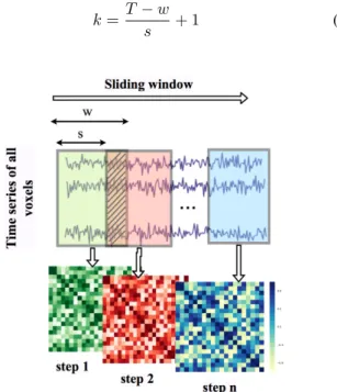
The fMRI functional connectivity has many applications in brain studies [4]–[10]. One of the well known applications is constructing brain functional network. In order to construct such a network each voxel of the brain is considered as a vertex in graph and is connected to another voxel if there is high correlation between their time series. Properties of functional brain networks have revealed many facts about the function of the brain. Another well known application of functional connectivity is learning internal patterns and using them as discriminative features for distinguishing healthy subjects from patients. In earlier studies, the functional connectivity was considered to be static but recent studies have shown that it has a dynamic nature and fluctuates over time which introduced the concept of dynamic-functional connectivity [11]. One way to construct the dynamic-functional connectivity of the brain is by the sliding window framework. In this approach a temporal window with length w starts from the first element of time series (t = 0) and covers consecutive time points up to w. All pairwise correlations between regions of the brain are computed considering time points in range [0, w]. Next, the window slides by step size s, covering time points in range
[s, s+w]. This process is continued until the window reaches the end of the time series. Fig. 1 shows the general overview of this process.
times that window can slide is computed by the following equation:
k=T−w
s + 1 (3)
Fig. 1: Sliding window framework for generating dynamic-functional connectivity with window sizewand step size s
One challenge for computing pairwise correlation coeffi-cients is its overall running time specially for voxel-based studies since there are thousands of voxels in a typical fMRI data. Many studies have targeted this problem and came up with parallel computing strategies in order to reduce the running time [12]–[16]. In case of dynamic-functional connectivity this problem is scaled since multiple correlation matrices are generated based on parameterswands. Most of proposed parallel computing techniques are designed for the purpose of computing static functional connectivity. To the best of our knowledge there is only one GPU-based technique proposed by [17] but it only focuses on computing dynamic-functional connectivity among regions of the brain and does not offer any solution for handling large voxel-based corre-lation matrices. Besides the time consuming nature, massive space requirement is another concern about DFC analysis in voxel level. Considering N voxels in fMRI data, pairwise correlations has O(N2) space complexity. Let’s assume an
example of fMRI data containing N = 30k voxels with length 150 which is a common size in fMRI study. Based on symmetric property of Pearson’s correlation, computing
N(N−1)
2 correlations covering strictly upper triangle part
instead of whole correlation matrix (N2) suffices which for this example needs 1.67 GB of memory. Now considering the window-based approach with window size w = 80 and step size s = 1, as given in equation 3, 71 sets of correlation coefficients need to be computed which needs 118.5 GB memory to store all correlations which is much larger than available memory in mid-sized labs.
Previously, we proposed a GPU-based technique called
Fast-GPU-PCC [12] for computing pairwise Pearson’s correlations considering the whole time series. This algorithm computes the strictly upper triangle part of the correlation matrix. Con-sidering the time and space consuming issues of dynamic func-tional connectivity, in this paper we propose GPU-DFC which is an extension of Fast-GPU-PCC for computing dynamic-functional connectivity.
A. GPU architecture and CUDA programming model Graphics Processing Units (GPUs) play an important role in general-purpose scientific computing in different fields by accelerating time consuming part of the code [18]. A GPU consists of an array of streaming multiprocessors (SMs) each containing several cores. Hundreds of threads run on each core simultneously based on Single Instruction Multiple Threads (SIMT) strategy. NVIDIA provides a GPU programming interface called CUDA which allows programmers to use CUDA-enabled GPUs to perform general purpose computing tasks [19]. GPU threads perform the instructions provided to them by a kernel function. A group containing 32 consecutive threads is called a warp. Threads inside the same warp perform the same instruction at the same time. In programming per-spective, maximum of 1024 threads are organized into groups called blocks which can be organized into one or two dimen-sion grids. GPU contains different types of memory such as Global memory, Shared memory, Texture memory and Local memory. Data transferred from CPU to GPU resides in Global memory and is accessible by all threads. Shared memory is on-chip memory which is accessible by all threads in the same block and is faster than Global memory. Using Shared memory is beneficial when threads inside the block need to access the data multiple times. Transferring data between CPU and GPU is a slow process because of low bandwidth between CPU and GPU memory and overheads associated to each transfer which can deteriorate overall performance. Hence, it is important to reduce the data transfers between CPU and GPU as much as possible. Another important point for designing a GPU based technique is ensuring coalesced global memory accesses which happens when threads inside a warp access to adjacent memory locations.
Efficient CUDA libraries such as cuBLAS [20], cuS-PARSE [21] and cuSOLVER [22] for performing different matrix operation and factorization are provided by NVIDIA. In this study we exploited some functions from these libraries. Contributions of the paper: The major contributions of this paper are as follows:
1) We propose a GPU-based technique for computing dy-namic functional connectivity of fMRI data which is an essential tool for dynamic connectomics.
2) In order to mitigate the memory requirements for storing large correlation matrices, we propose a sparsification strategy that reduces the number of correlations by removing weak values.
3) We propose another strategy based on matrix decom-position for decomposing each correlation matrix into
small matrices which significantly reduces the space needed for storing each correlation matrix.
Organization of the paper: This paper is organized as follows: In section 1 we briefly review the Fast-GPU-PCC technique and how we expand it to compute dynamic func-tional connectivity. In section 2 we describe the sparsification technique for reducing the size of correlation matrices. In section 3 we describe our second strategy for reducing the space requirement by using matrix decomposition. Section 4 describes the overall framework of GPU-DFC. In section 5 we discuss the experiments and results and section 6 includes conclusion and future work of this study.
I. COMPUTING DYNAMIC FUNCTIONAL CONNECTIVITY BASED ONFAST-GPU-PCCALGORITHM
In Fast-GPU-PCC algorithm, the first step is to normalize time series of all voxels as given in equation 2. This process is performed on CPU, then the normalized time series are transferred to the GPU. We assume U denotes the matrix containing the normalized time series. Therefore, multiplying
U to its transposeUT will generate correlation matrixS. The upper triangle part of matrixS is then extracted and stored in row major order in array C using algorithm 1.
In this algorithm, one GPU thread is assigned to one cell of Algorithm 1 Kernel function for extracting ordered upper triangle part of the correlation matrix
Input:n×n correlation matrix S
Output: Ordered correlation array C of sizen(n−1)/2
1: idx=blockDim.x∗blockIdx.x+threadIdx.x
2: i=idx/n
3: j=idx%n
4: if i < j andi < nandj < nthen
5: k1=i×n− i×(i+ 1) 2 +j−i 6: k2=j×n+i 7: C[k1−1] =S[k2] 8: end if
correlation matrix, if this cell is located in strictly upper trian-gle part, its value is copied to specific location in correlation arrayC. Sometimes the size of correlation matrix is larger than the available GPU memory. In such cases the algorithm divides the time series matrix to smaller blocks, computes a chunk of correlation matrix, extract the elements in upper triangle, transfer them back to CPU and starts another chunk.
For computing dynamic functional connectivity, these steps should be repeated each time the window slides over the time series. So instead of normalizing all time series in CPU and transfer them to GPU for each slide, in the proposed approach we transfer the original time series to GPU in the beginning and normalize the section of time series in the window using the algorithm 2.
In this algorithm each GPU block contains 32 threads and is responsible for normalizing one time series. By using
Algorithm 2 Kernel function for normalizing part of time series in window w
Input: Ann×t matrixU of time series data, Windows length w, start positionst (starting position of window) Output: Normalized matrixU0
1: slide=dwindow_size/32e
2: start=blockIdx.x∗t+st
3: Copy time series (starting at st) of window w to shared memory sh
4: fori= 0 toslidedo
5: psum+ =sh[threadIdx.x+ (i×32)]
6: end for
7: sum = adding up local_sum of threads in a group using shuffle warp reduce technique
8: ifthreadIdx.x= 0then 9: sh[windowsize] =sum/w 10: end if 11: avg= 0 12: fori= 0 toslidedo 13: index=threadIdx.x+ (i×32) 14: if index < wthen
15: avg=avg+ (sh[index]−sh[windowsize])2
16: sh[index]−=sh[windowsize]
17: end if
18: end for
19: sum = adding up avg values
20: ifthreadIdx.x= 0then 21: sh[windowsize] =sqrt(sum) 22: end if 23: idx=blockIdx.x∗w 24: fori= 1 toslidedo 25: index=threadIdx.x+ (i×32) 26: if index < wthen
27: U0[idx+ (index)] =sh[index]/sh[w] 28: end if
29: end for
32 threads or a warp, global memory coalescing is ensured since threads access to consecutive memory locations. Also, computing summation of all elements inside the window can be easily done by using shuffle warp reduce technique without needing extra memory for storing temporary values. In the beginning of the algorithm, threads of each block find the starting position of the window and copy its corresponding elements into shared memory (line 2 and 3). In line 4 to 10, the average of windowed time series is computed by threads and is stored in shared memory. Threads compute the numerator and denominator of equation 2 by subtracting average value from each time point and computing the L2 norm (line 12 to end).
After this algorithm completes, the preprocessed values are stored in matrix U0 in GPU global memory. The next step is multiplying matrix U0 to its transpose which results the correlation matrixS. The upper triangle of this matrix can be
extracted using algorithm 1.
II. SPARSIFICATION METHOD FOR REDUCING THE SIZE OF CORRELATION MATRICES
In case of voxel-based analysis or in scenarios in which many regions of interest are considered, usually the size of correlation matrices are very large and even after extracting upper triangle part they consume a lot of memory. On the other hand transferring large correlation matrices from GPU to CPU would be time consuming considering slow PCIe cable connecting CPU memory to GPU memory. One way to reduce the memory requirement is making the correlation matrices sparse by replacing correlations below a threshold to zero and only keeping nonzero values using a sparse data structure like Compressed Sparse Row (CSR) format. The idea of sparsifying fMRI correlation matrix has been used by Zhao et al [16] for reducing size of one correlation matrix in static functional connectivity analysis. CSR format uses three arrays for storing nonzero values, their column and row indices. Since correlation matrix is symmetric, we only save nonzero elements in upper triangle by zeroing out all elements in lower triangle and diagonal using a sparsification kernel which is shown in algorithm 3 (Same result can be achieved by zeroing out elements in upper triangle instead of lower triangle). In this algorithm each GPU thread checks one Algorithm 3 Sparsifying dense correlation matrix to sparse matrix
Input:n×n correlation matrix S and thresholdz
Output: Sparse correlation matrixS with non-zero values in uppr triangle
1: idx=blockDim.x∗blockIdx.x+threadIdx.x
2: i=idx/n
3: j=idx%n
4: if (i > j||S[idx]< z)andi < nandj < nthen
5: S[idx] = 0
6: end if
cell of correlation matrix at a time. If this cell is located in upper triangle and its value is above the threshold, it does not change it otherwise sets its value to zero. After this step, the sparse correlation matrix is stored in CSR format. Eliminating weak correlations and only keeping strong correlations above a predefined threshold is a common practice in brain network construction [23], [24].
III. REDUCING THE SIZE OF DENSE CORRELATION MATRIX USING APPROXIMATE LOW RANK MATRIX DECOMPOSITION
Although making correlation matrix sparse by removing correlations below a threshold and storing it in CSR for-mat reduces the memory requirement of correlation for-matrix significantly, it causes loosing some information about the brain connectivities. Specially negative connections which can be useful for understanding functional connectivity structure of brain disorders. In order to keep those information while reducing the size of dense correlation matrices, we exploit
a matrix decomposition strategy. Matrix decomposition or matrix factorization techniques like Singular Value Decom-position (SVD) are well known techniques for dimensionality reduction and compression [25], [26]. For example, truncated SVD provides low rank approximation of a matrix by only keeping its largest singular values and corresponding singular vectors which helps reducing the size of the matrix. Matrix decomposition techniques can be time consuming applying on large scale problems. HALKO et al [27] proposed a framework for constructing randomized algorithms to perform different matrix decomposition tasks. Based on their framework, low-rank approximation of a given m×nmatrix Ais proceeded in two steps. In the first step, an approximation to the range of A is computed by obtaining matrixQsuch that:
A≈QQ>A (4)
The goal is to compute matrix Q with m rows and l or-thonormal columns such that l < n. In second step, matrix
Q is used for computing matrix factorization like SVD. In this study we only utilize the first step and decompose the correlation matrix into matrices Q and B (Q>A). Since Q
andB containl column/rows andl < n, the total size needed for storing matrices B and Qwould be l(m+n)instead of
mn. To compute matrix Q, first the range of matrix A is approximately spanned by performingy=A×σin whichσis ann×lGaussian random matrix. Finally anm×lmatrixQis computed by taking QR decomposition of matrixy(y=QR). The following pseudocode shows the steps that we perform to factorize each correlation matrix to matrices Q and B. By using this approach each correlation matrix A can be Algorithm 4 Reducing required space in dynamic-functional connectivity by performing matrix decomposition
Input: n×ncorrelation matrix S and integerl Output: n×l matrixQandl×nmatrix B
1: Generaten×l Gaussian random matrixσ
2: y=S×σ
3: Q, R=QR(y)
4: B=Q>×S
5: retrunB andQ
decomposed into two matrices B and Q with smaller sizes. As we will see in the next section, choosing value oflsmaller thanT (length of time series) provides good approximation of correlation matrix with very small error. Also reconstructing correlation matrix fromQandRwhich is simplyQ×B, takes shorter time than computing correlation matrix from scratch since QandR are smaller than time series matrix and there is no need to normalize them before matrix multiplication.
IV. OVERAL FRAMEWORK OFGPU-DFC
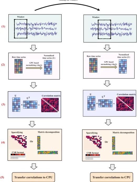
Considering all proposed methods in last sections, the over-all framework of GPU-DFC is shown in algorithm 5. Based on this algorithm, by sliding the window over time series, values inside the window are normalized using algorithm
Fig. 2: Sliding window framework for generating dynamic-functional connectivity and strategies for reducing the size of correlation matrices. In step 1 the window slides over the time series. In step 2, the algorithm normalizes the time series values inside the window using algorithm 2. Step 3 performs the matrix multiplication to compute correlation matrix. In step 4 the memory reduction technique is applied (either sparsification or matrix decomposition). In section 5 the correlation values are transferred to CPU.
Algorithm 5 Computing dynamic funcional connectivity based on GPU-DFC
Input:n×t fMRI data consisting ofnvoxels with time series of lengtht, Window sizewand step size s Output: (t−w)/s+ 1 correlation matrices
1: num= (t−w)/s+ 1
2: Copy fMRI data from CPU to GPU
3: if Enough GPU memorythen
4: fori= 0to num do
5: U ←Preprocess data inside windowi by algorithm 2
6: corr=U×UT
7: Extract upper triangle using algorithm 1
8: end for
9: Transfer all correlations to CPU
10: else
11: fori= 0to num do
12: U ←Preprocess data inside windowi by algorithm 2
13: corr=U×UT
14: if Approach 1then
15: Us←Sparsify correlation matrix using algorithm 3
16: A,IA,J A←CSR(Us)
17: else
18: Q, B←Apply algorithm 4 on corr
19: end if
20: Transfer the results (Q,B) or (A,IA,J A) to CPU
21: end for
22: end if
2. If memory requirement for storing all correlations is not an issue, all correlation matrices can be computed in GPU and transfer to CPU at the end. Otherwise, either matrix decomposition or sparsification techniques can be utilized. The choice of selecting these techniques depends on the application for which correlations are computed. If the goal is working with high correlation values (above a threshold), then negative and weak correlations are not needed and therefore, the sparsification methods can be chosen. On the other hand if the information of all pairwise correlations are needed, then the matrix decomposition technique can be used instead. This process is shown in Fig. 2.
V. EXPERIMENTS AND RESULTS
In this section we evaluate the performance of the proposed frameworks and compare it with two other baselines. The first baseline is sequential version of computing dynamic-functional connectivity on CPU. The second algorithm is GPU-PCC which is a GPU-based technique we previously proposed for computing pairwise Pearson’s correlation [28]. This algorithm was designed to compute one correlation matrix considering the whole time series. In order to make it work for dynamic correlation computation, we repeated this
algorithm inside a loop such that in each iteration pairwise correlations over one window is computed.
All the experiments of this section are performed on a Linux server with Ubuntu Operating System version 14.04. This server includes two Intel Xeon E5 2620 processors with clock speed 2.4 GHz, 48 GBs RAM and NVIDIA Tesla K40c Graphic Processing Unit. This GPU contains 15 Streaming Multiprocessors each consists of 192 CUDA cores and 11520 MBytes global memory. CUDA version 8, g++ version 4.4.8 are utilized for performing experiments. Optimization level -O2 was used for compiling codes that run on CPU.
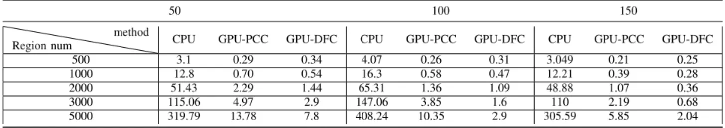
A. Experiment 1: Computing DFC on region based data In the first experiment we evaluated the performance of computing dynamic-functional connectivity on regions of the brain. Since the number of regions in region based analysis are usually small, memory requirement is not a concern. We per-formed this experiment on synthetic fMRI data by generating random floating-point numbers in range -6 to 6 as intensity of each voxel. Since the goal of this experiment is only measuring the running time of the algorithm and intensity values are usually represented by floating-point numbers, almost the same running time can be obtained by using random floating-point numbers compared to real data. We tested different region numbers (500, 1000, 2000, 3000, 5000) each having a time series of length 200 and considered different window sizes (50, 100, 150). Table I compares the running time of different approaches. As can be observed from the table, by increasing number of regions, the proposed method performs faster that other techniques. By increasing the length of window, the number of correlation matrices that needs to be computed is decreased so the running time of all techniques are reduced. B. Sparsification technique
In this experiment we applied the proposed method on real voxel-based fMRI data. The fMRI data that we used is part of preprocessed samples provided by ADHD-200 initiative [29]. It contains 30697 voxels with time series of length 257. Pairwise correlations of this dataset need 1.75 GB memory (only correlations in strictly upper triangle), considering window size of length 150 and step size 1, 108 correlation matrices need to be stored which requires 189 GB of memory. This is much more than available memory in our system and many other modern computers, so we applied the sparsification strategy to reduce the size of correlation matrices. Table II shows the running time of applying the algorithm on real data based on different thresholds and window sizes. Other baselines that are stated in experiment 1 (CPU-version and GPU-PCC) don’t use any method for reducing the size of correlation matrices so we didn’t include them in this experiment. Based on the result, increasing the value of the threshold, correlation matrices become sparser and fewer elements are stored in CSR format. This can be observed from table II such that higher thresholds have shorter running times for all values of w.
TABLE I: Running time (seconds) of applying different techniques on region based data
50 100 150
Region num
method
CPU GPU-PCC GPU-DFC CPU GPU-PCC GPU-DFC CPU GPU-PCC GPU-DFC
500 3.1 0.29 0.34 4.07 0.26 0.31 3.049 0.21 0.25
1000 12.8 0.70 0.54 16.3 0.58 0.47 12.21 0.39 0.28
2000 51.43 2.29 1.44 65.31 1.36 1.09 48.88 1.07 0.36
3000 115.06 4.97 2.9 147.06 3.85 1.6 110 2.19 0.68
5000 319.79 13.78 7.8 408.24 10.35 2.9 305.59 5.85 2.04
TABLE II: Running time (seconds) of different window size (w) and threshold values (θ)
θ W 50 100 150 0.3 148 86.33 53.561 0.5 81.56 53.19 40.54 0.7 63.46 51.76 38.92 l 64 (T/4) 85 (T/3) 128 (T/2) 257 (T) MAE 0.002 1.3e-07 5.8e-08 3.77e-08 compression-ratio 239 180 119 59
TABLE III: Mean absolute error and compression ratio based on different ranks l
C. Matrix decomposition based technique
In order to evaluate the effectiveness of matrix decompo-sition for reducing the memory requirements of correlation matrices, we applied the matrix decomposition strategy on real voxel-based fMRI data. In the first experiment we applied the algorithm 4 on real fMRI data we used in the last experiment and constructed the correlation matrix considering the whole time series. Different ranks l are tested for low rank matrix decomposition. After applying this algorithm matricesQand
B are stored instead of the original correlation matrix. Com-pression ratio of storingQandRinstead of whole correlation matrix can be computed using the following equation:
CR= n×n 2×n×l =
n
2×l (5)
In this equation, numerator (n×n) represents the size of original matrix and denominator (2×n×l) represents the space needed for storing matrix Q (n×l) and B (l×n). By performing low rank decomposition some amount of data might be lost. In order to see how low rank decomposition can change the values of correlations, we reconstructed the correlation matrix by multiplying matricesQ and B to each other and computed mean absolute error (MAE) of the re-constructed correlations. Table III shows MAE and CR values based on different ranksl. In another experiment we used the actual and reconstructed correlations as features for classify-ing subjects sufferclassify-ing from Autism spectrum disorder from healthy subjects. We used NYU dataset provided by ABIDE initiative [30]. This dataset contains preprocessed fMRI data provided by ABIDE initiative. The data that we used from this dataset contains 75 Autism and 98 healthy subjects. Each
fMRI data is divided into 200 regions generated using spatially constrained spectral clustering algorithm. Length of each time series (T) is equal to 175. We used the upper triangle part of the200×200pairwise correlation matrix of each subject as its features and used Multi-layer Perceptron for classification. In order to see how losing the data after matrix decomposition affects the result of classification, we compared the results of using actual correlations versus using reconstructed cor-relations (computed by multiplying decomposed matrices Q
andB). For matrix decomposition, we setl=58(T /(3)). The mean absolute error of reconstructed correlations is equal to 0.003. We repeated 5-fold Cross-Validation approach 10 times and computed the average accuracy, specificity and sensitivity. Based on the results shown in table IV, reconstructed
correla-Accuracy Sensitivity Specificity Actual Corrs 61.9 51.7 69.7 Reconstructed corrs 61.5 52.1 68.5
TABLE IV: Accuracy, sensitivity and specificity of MLP classification with actual and reconstructed correlations tions got almost the similar result as actual correlations which shows that by applying matrix decomposition to correlation matrices important information about functional structure of the data is preserved.
In the final experiment we measured the running time of computing dynamic-functional connectivity and applying the matrix decomposition technique to correlation matrices using real data we used in subsection B. Table V shows the running time using window size equal to 150 and different ranks l. Based on the results, by increasing rank l, the running time
l 50 75 100 Running time 125.8 137.16 142.2
TABLE V: Running time (seconds) of computing dynamic functional connectivity with w = 150 and using matrix decomposition strategy based on different ranksl.
increases slightly. Overall, the results indicate the scalability and efficiency of using matrix decomposition technique for reducing the size of correlation matrices.
VI. CONCLUSION ANDFUTURE WORK
In this paper we proposed a GPU-based framework called GPU-DFC for computing dynamic-functional connectivity of
fMRI data in both region and voxel levels. Since the number of voxels in fMRI data can be huge and results in large correlation matrices, we proposed two techniques to reduce the memory requirements of correlation matrices. The first approach is based on sparsifying correlation matrices and storing them in CSR format and the other one is based on decomposing each correlation matrix into smaller matrices. GPU-DFC achieved around 2 times speed up for computing dynamic correlations comparing to another GPU-based technique which is used for computing static correlation matrix and more than 40 times comparing to sequential CPU version. Our proposed matrix decomposition technique reduces the size of correlation matrices more than 100 times. Reconstructed values from decomposed matrices show small mean absolute error and using them in real applications like classification show almost the same result as using actual correlations.
For the future direction of this study we will focus on design-ing GPU-based pipelines for large scale dynamic-functional connectivity based applications like classification and graph mining techniques.
ACKNOWLEDGMENT
This research was supported by the National Institute Of General Medical Sciences (NIGMS) of the National Institutes of Health (NIH) under Award Number R15GM120820. The content is solely the responsibility of the authors and does not necessarily represent the official views of the National Institutes of Health. Fahad Saeed was additionally supported by National Science Foundation grants NSF CAREER ACI-1651724. We would also like to acknowledge the donation of a K-40c Tesla GPU and TITANXp GPU from NVIDIA which was used for all GPU-based experiments performed in this paper.
REFERENCES
[1] R. C. Craddock, R. L. Tungaraza, and M. P. Milham, “Connectomics and new approaches for analyzing human brain functional connectivity,”
Gigascience, vol. 4, no. 1, p. 13, 2015.
[2] M. A. Lindquistet al., “The statistical analysis of fmri data,”Statistical Science, vol. 23, no. 4, pp. 439–464, 2008.
[3] C. Chang and G. H. Glover, “Time–frequency dynamics of resting-state brain connectivity measured with fmri,”Neuroimage, vol. 50, no. 1, pp. 81–98, 2010.
[4] T. Eslami and F. Saeed, “Similarity based classification of adhd using singular value decomposition,” inProceedings of the ACM International Conference on Computing Frontiers 2018. ACM, 2018.
[5] X. Liang, J. Wang, C. Yan, N. Shu, K. Xu, G. Gong, and Y. He, “Effects of different correlation metrics and preprocessing factors on small-world brain functional networks: a resting-state functional mri study,”PloS one, vol. 7, no. 3, p. e32766, 2012.
[6] Y. Zhang, H. Zhang, X. Chen, S.-W. Lee, and D. Shen, “Hybrid high-order functional connectivity networks using resting-state functional mri for mild cognitive impairment diagnosis,”Scientific reports, vol. 7, no. 1, p. 6530, 2017.
[7] X. Zhao, Y. Liu, X. Wang, B. Liu, Q. Xi, Q. Guo, H. Jiang, T. Jiang, and P. Wang, “Disrupted small-world brain networks in moderate alzheimer’s disease: a resting-state fmri study,”PloS one, vol. 7, no. 3, p. e33540, 2012.
[8] D. Godwin, A. Ji, S. Kandala, and D. Mamah, “Functional connectivity of cognitive brain networks in schizophrenia during a working memory task,”Frontiers in psychiatry, vol. 8, p. 294, 2017.
[9] H.-C. Baggio, R. Sala-Llonch, B. Segura, M.-J. Marti, F. Valldeoriola, Y. Compta, E. Tolosa, and C. Junqué, “Functional brain networks and cognitive deficits in parkinson’s disease,”Human brain mapping, vol. 35, no. 9, pp. 4620–4634, 2014.
[10] R. C. Craddock, G. A. James, P. E. Holtzheimer, X. P. Hu, and H. S. Mayberg, “A whole brain fmri atlas generated via spatially constrained spectral clustering,”Human brain mapping, vol. 33, no. 8, pp. 1914– 1928, 2012.
[11] M. G. Preti, T. A. Bolton, and D. Van De Ville, “The dynamic functional connectome: state-of-the-art and perspectives,” Neuroimage, vol. 160, pp. 41–54, 2017.
[12] T. Eslami and F. Saeed, “Fast-gpu-pcc: A gpu-based technique to compute pairwise pearson’s correlation coefficients for time series data—fmri study,”High-throughput, vol. 7, no. 2, p. 11, 2018. [13] J. D. Lusher, J. X. Ji, and J. M. Orr, “Implementation of
high-performance correlation and mapping engine for rapid generation of brain connectivity networks from big fmri data,” in2018 40th Annual International Conference of the IEEE Engineering in Medicine and Biology Society (EMBC). IEEE, 2018, pp. 1032–1036.
[14] J. Lusher, J. Ji, and J. Orr, “High-performance correlation and mapping engine for rapid generating brain connectivity networks from big fmri data,”Journal of computational science, vol. 26, pp. 157–164, 2018. [15] Y. Wang, H. Du, M. Xia, L. Ren, M. Xu, T. Xie, G. Gong, N. Xu,
H. Yang, and Y. He, “A hybrid cpu-gpu accelerated framework for fast mapping of high-resolution human brain connectome,”PloS one, vol. 8, no. 5, p. e62789, 2013.
[16] K. Zhao, H. Du, and Y. Wang, “A gpu-accelerated framework for fast mapping of dense functional connectomes,” 2017.
[17] D. Akgün, Ü. Sako˘glu, J. Esquivel, B. Adinoff, and M. Mete, “Gpu accelerated dynamic functional connectivity analysis for functional mri data,”Computerized Medical Imaging and Graphics, vol. 43, pp. 53–63, 2015.
[18] M. G. Awan, T. Eslami, and F. Saeed, “Gpu-daemon: Gpu algorithm design, data management & optimization template for array based big omics data,”Computers in biology and medicine, vol. 101, pp. 163–173, 2018.
[19] J. Sanders and E. Kandrot, CUDA by example: an introduction to general-purpose GPU programming. Addison-Wesley Professional, 2010.
[20] NVIDIA, “cublas,” http://docs.nvidia.com/cuda/cublas/index.html# #axzz4VJn7wpRs, Mar. 2017.
[21] ——, “cusparse,” https://docs.nvidia.com/cuda/cusparse/index.html, Oct. 2018.
[22] ——, “cusolver,” https://docs.nvidia.com/cuda/cusolver/index.html, Nov. 2018.
[23] C. Bordier, C. Nicolini, and A. Bifone, “Graph analysis and modularity of brain functional connectivity networks: searching for the optimal threshold,”Frontiers in neuroscience, vol. 11, p. 441, 2017.
[24] T. Uehara, T. Yamasaki, T. Okamoto, T. Koike, S. Kan, S. Miyauchi, J.-i. Kira, and S. Tobimatsu, “Efficiency of a “small-world” brain network depends on consciousness level: a resting-state fmri study,”Cerebral Cortex, vol. 24, no. 6, pp. 1529–1539, 2013.
[25] L. Cao, “Singular value decomposition applied to digital image process-ing,”Division of Computing Studies, Arizona State University Polytech-nic Campus, Mesa, Arizona State University polytechPolytech-nic Campus, pp. 1–15, 2006.
[26] J.-J. Wei, C.-J. Chang, N.-K. Chou, and G.-J. Jan, “Ecg data compression using truncated singular value decomposition,”IEEE Transactions on Information Technology in Biomedicine, vol. 5, no. 4, pp. 290–299, 2001. [27] N. Halko, P.-G. Martinsson, and J. A. Tropp, “Finding structure with randomness: Probabilistic algorithms for constructing approximate ma-trix decompositions,”SIAM review, vol. 53, no. 2, pp. 217–288, 2011. [28] T. Eslami, M. G. Awan, and F. Saeed, “Gpu-pcc: A gpu based technique
to compute pairwise pearson’s correlation coefficients for big fmri data,” in Proceedings of the 8th ACM International Conference on Bioinformatics, Computational Biology, and Health Informatics. ACM, 2017, pp. 723–728.
[29] P. Bellec, C. Chu, F. Chouinard-Decorte, Y. Benhajali, D. S. Margulies, and R. C. Craddock, “The neuro bureau adhd-200 preprocessed reposi-tory,”Neuroimage, vol. 144, pp. 275–286, 2017.
[30] C. Craddock, Y. Benhajali, C. Chu, F. Chouinard, A. Evans, A. Jakab, B. S. Khundrakpam, J. D. Lewis, Q. Li, M. Milham et al., “The neuro bureau preprocessing initiative: open sharing of preprocessed neuroimaging data and derivatives,”Neuroinformatics, 2013.