MULTIOBJECTIVE PARTICLE SWARM OPTIMIZATION: INTEGRATION OF DYNAMIC POPULATION AND MULTIPLE-SWARM CONCEPTS
AND CONSTRAINT HANDLING
By
WEN FUNG LEONG
Bachelor of Science in Electrical Engineering Oklahoma State University
Stillwater, Oklahoma 2000
Master of Science in Electrical Engineering Oklahoma State University
Stillwater, Oklahoma 2002
Submitted to the Faculty of the Graduate College of the Oklahoma State University
in partial fulfillment of the requirements for
the Degree of
DOCTOR OF PHILOSOPHY December, 2008
MULTIOBJECTIVE PARTICLE SWARM OPTIMIZATION: INTEGRATION OF DYNAMIC POPULATION AND MULTIPLE-SWARM CONCEPTS
AND CONSTRAINT HANDLING
Dissertation Approved: Dr. Gary G. Yen Dissertation Adviser Dr. Guoliang Fan Dr. Carl D. Latino Dr. R. Russell Rhinehart Dr. A. Gordon Emslie Dean of the Graduate College
ACKNOWLEDGMENTS
First and foremost, I would like to express my deepest gratitude to my advisor, Professor Gary G. Yen. Over the course of this study, he has provided his insightful guidance, continued motivation and unlimited patience in guiding my writing progress. Furthermore, he has also given me other opportunities including conference and professional experiences, and financial assistance.
My heartfelt appreciation to my committee members, Professor Guoliang Fan, Professor Carl D. Latino, and Professor R. Russell Rhinehart, for their time, valuable feedback, and constructive feedback.
Many thanks to Dr. Huantong Geng, from Nanjing University of Information Science and Technology, for sharing the source code of his published journal [164].
To my past and present colleagues of Intelligent Systems and Control Laboratory (ISCL), Sangameswar Venkatraman, Daghan Acay, Pedro Gerbase de Lima, Michel Goldstein,Monica Wu Zheng, Xiaochen Hu, Yonas G. Woldesenbet, Biruk G. Tessema, Kumlachew Woldemariam, Moayed Daneshyari, Ashwin Kadkol, Yared Nesrane, and Nardos Zewde, I thank you all for the constructive discussions, the brainstorming sessions, friendship and help. I have had the pleasure of working with Xin Zhang and I thank her for valuable inputs and collaborative work.
(Chew, Bun, Ting, and Zhou) for being patience, giving me their unconditional love, financial and moral supports. Finally, my special thanks to my husband, Edmond J.O. Poh for his encouragement, love, and giving emotional supports.
TABLE OF CONTENTS Chapter Page 1. INTRODUCTION ...1 1.1 Motivation...1 1.2 Objective ...2 1.3 Contributions...5
1.4 Outline of the Dissertation ...6
2. MULTIOBJECTIVE OPTIMIZATION...9 2.1 Definition ...9 2.1.1 Pareto Optimization ...11 2.1.2 Example ...12 2.2 Optimization Methods ...13 2.2.1 Conventional Algorithms...14 2.2.2 Aggregating Approach...18
2.2.3 Multiobjective Evolutionary Algorithms (MOEAs)...18
2.2.3.1 General Concept...20
2.2.3.2 A Brief Tour of MOEAs ...20
2.3 Test Functions ...24
2.4 Performance Metrics ...25
3. SWARM INTELLIGENCE...29
3.1 Introducing Swarm Intelligence...29
3.1.1 Fundamental Concepts...30
3.1.2 Example Algorithms ...31
3.2 Modeling the Behavior of Bird Flock ...34
4. PARTICLE SWARM OPTIMIZATION...40
4.1 Brief History of Particle Swan Optimization...40
4.2 Standard PSO Equations ...43
4.3 The Generic PSO Algorithm...46
Chapter Page
4.4.1 Parameter Settings ...48
4.4.1.1 Inertial Weight ...48
4.4.1.2 Acceleration Constants ...50
4.4.1.3 Clipping Criterion ...51
4.4.2 Modifications of PSO Equations ...52
4.4.3 Neighborhood Topology...55
4.4.4 Multiple-swarm Concept in PSO ...58
4.4.4.1 Solving Multimodal Problems ...58
4.4.4.2 Tracking All Optima for Multimodal problems in Dynamic Environment ...60
4.4.4.3 Promoting Exploration and Diversity ...61
4.4.5 Other PSO Variations ...63
5. MULTIOBJECTIVE PARTICLE SWARM OPTIMIZATION (MOPSO) ...65
5.1 Particle Swarm Optimization Algorithm for MOPs ...65
5.2 General Framework of MOPSO ...67
5.2.1 External Archive ...69
5.2.2 Global Leaders Selection Mechanism ...72
5.2.3 Personal Best Selection Mechanism ...80
5.2.4 Incorporation of Genetic Operators ...82
5.2.5 Incorporation of Multiple Swarms...84
5.2.6 Other MOPSO Designs...86
6. PROPOSED ALGORITHM 1: DYNAMIC MULTIOBJECTIVE PARTICLE SWARM OPTIMIZATION (DMOPSO) ...88
6.1 Introduction...89
6.2 Proposed Algorithm Overview ...91
6.3 Implementation Details...94
6.3.1 Cell-based Rank Density Estimation Scheme...94
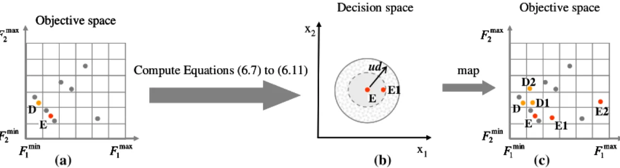
6.3.2 Perturbation Based Swarm Population Growing Strategy...99
6.3.3 Swarm Population Declining Strategy...104
6.3.4 Adaptive Local Archives and Group Leader Selection Procedures...111
6.4 Comparative Study...114
6.4.1 Test Function Suite ...114
6.4.2 Parameter Settings ...116
6.4.3 Selected Performance Metrics ...116
6.4.4 Performance Evaluation of DMOPSO against the selected MOPSOs .119 6.4.5 Investigation of Computational Cost of DMOPSO with Selected MOPSOs ...128
Chapter Page 7. PROPOSED ALGORITHM 2: DYNAMIC MULTIPLE SWARMS IN
MULTIOBJECTIVE PARTICLE SWARM OPTIMIZATION (DSMOPSO) ...130
7.1 Introduction...131
7.2 Proposed Algorithm Overview ...133
7.3 Implementation Details...135
7.3.1 Cell-based Rank Density Estimation Scheme...135
7.3.2 Identify Swarm Leaders ...136
7.3.3 Update Local Best of Swarms...136
7.3.4 Archive Maintenance ...137
7.3.5 Particle Update Mechanism (Flight)...139
7.3.6 Swarm Growing Strategy...143
7.3.7 Swarm Declining Strategy ...150
7.3.8 Objective Space Compression and Expansion Strategy ...153
7.4 Comparative Study...157
7.4.1 Experimental Framework...159
7.4.2 Selected Performance Metrics ...159
7.4.3 Performance Evaluation...160
7.4.4 Comparison in Number of Fitness of Evaluation ...169
7.4.5 Sensitivity Analysis ...170
8. PROPOSED PSO AND MOPSO FOR CONSTRAINED OPTIMIZATION...175
8.1 Introduction...175
8.2 Related Works...177
8.3 Proposed Approach...183
8.3.1 Transform a COP into an Unconstrained Bi-objective Optimization Problem ...183
8.3.2 Proposed PSO Algorithm to Solve COPs ...185
8.3.2.1 Update Personal Best (Pbest) Archive ...186
8.3.2.2 Update Feasible and Infeasible Global Best Archive ...189
8.3.2.3 Particle Update Mechanism ...191
8.3.2.4 Mutation Operator...193
8.3.3 Proposed Constrained MOPSO to Solve CMOPs ...196
8.3.3.1 Update Personal Best Archive ...198
8.3.3.2 Update Feasible and Infeasible Global Best Archive ...199
8.3.3.3 Global Best Selection...201
8.3.3.4 Mutation Operator...201
8.4 Comparative Study...203
8.4.1 Experiment 1: Performance Evaluation of the Proposed PSO for COPs.... ...203
Chapter Page
8.4.1.2 Simulation Results and Analysis ...205
8.4.2 Experiment 2: Performance Evaluation of the Proposed Constrained MOPSO...208
8.4.2.1 Experimental Framework...208
8.4.2.2 Selected Performance Metrics ...210
8.4.2.3 Performance Evaluation...211
9. CONCLUSION AND FUTURE WORKS ...221
9.1 Dynamic Population Size and Multiple-swarm Concepts ...221
9.2 Constraint Handling ...225
LIST OF TABLES
Table Page
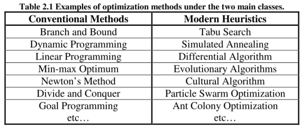
2.1 Examples of optimization methods under the two main classes...13 5.1 Comparison between a typical EA and PSO...66 6.1 The six test problems used in this study. All objective functions are to be
minimized ...115 6.2 Parameter configurations for five selected MOPSOs ...116 6.3 Parameter configurations for DMOPSO with number of iterations is based
upon 20,000 evaluations ...117 6.4 The computed additive binary epsilon indicator,Iε+
(
A,B)
, for all combinationof H1, H2, and P as shown in Figure 6.17 ...118 6.5 The distribution of IH values tested using Mann-Whitney rank-sum Test
[144].The table presents the z values and p-values with respect to the alternative hypothesis (i.e., p-value < α=0.05) for each pair of DMOPSO and a
selected MOPSO. In each cell, both values are presented in a bracket: (z value, p-value). The distribution of DMOPSO is significantly difference or better than those selected MOPSO unless stated ...121 6.6 The distribution of Iε+ values tested using Mann-Whitney rank-sum Test
[144].The table presents the z values and p-values with respect to the alternative hypothesis (i.e., p-value < α=0.05) for each pair of DMOPSO and a
selected MOPSO. In each cell, both values are presented in a bracket like this: (z value, p-value). For simplicity, DMOPSO is represented by A, and algorithms B1 to B5 are referred to as OMOPSO, MOPSO, cMOPSO, sMOPSO, and NSPSO, respectively. The distribution of DMOPSO is significantly difference or better than those selected MOPSO unless stated... ...122 6.7 Average number of evaluations required per run for all test problems from all selected algorithms and DMOPSO to achieve GD =0.001...127
Table Page 7.1 Parameter configurations for existing MOPSOs and DSMOPSO...160 7.2 The distribution of IH values tested using Wilcoxon rank-sum test. The table
presents the z values and p-values, i.e., presented in the brackets as (z value, p-value), with respect to the alternative hypothesis (i.e., p-value < α=0.05) for
each pair of DMOPSO and a selected MOPSO. Note that the distribution of DMOPSO is significantly difference or better than those selected MOPSO unless stated difference or better than those selected MOPSO unless stated ... ...163 7.3 The distribution of Iε+ values tested using Wilcoxon rank-sum test. The table
presents the z values and p-values with respect to the alternative hypothesis (i.e., p-value < α=0.05) for each pair of DMOPSO and a selected MOPSO. In
each cell, both values are presented in a bracket like this: (z value, p-value). For simplicity in naming, DSMOPSO is represented by A, and algorithms B1 to B3 are referred to as DMOPSO, MOPSO, and cMOPSO, respectively. The distribution of DMOPSO is significantly ...165 7.4 Average number of evaluations computed for the test problems to achieve GD =0.001 ...169 8.1 Brief summary of the effects of rf , pbest_cv, and gbest_cv on the second and third terms in Equation (8.6) ...193 8.2 Summary of main characteristics of the 19 benchmark functions ...204 8.3 Parameter configurations for the proposed PSO...204 8.4 Experimental results on the 19 benchmark functions with 50 independent runs. Note that the first column presents the test problem and its global optimal ...206 8.5 Comparison of the proposed algorithm with respect to SR[155], DOM+RVPSO [172], MSPSO [179], and PESO [182] on 13 benchmark functions. Note that the first column presents the test problem and its global optimal ...207 8.6 Parameter configurations for testing algorithms...208 8.7 The 14 benchmark CMOPs used in this study. All objective functions are to be minimized...209 8.8 Parameter setting for CTP2-CTP8 [183] ...210
Table Page 8.9 Summary of main characteristics of the 14 benchmark functions ...210 8.10 The distribution of IH values tested using Mann-Whitney rank-sum Test. The
table presents the z values and p-values with respect to the alternative hypothesis (i.e., p-value < α=0.05) for each pair of the proposed MOPSO and
a selected constrained MOEAs. In each cell, both values are presented in a bracket: (z value, p-value). The distribution of the proposed MOPSO is significantly different than those selected constrained MOEAs unless stated .... ...213 8.11 The distribution of Iε+ values tested using Mann-Whitney rank-sum Test. The
table presents the z values and p-values with respect to the alternative
hypothesis (i.e., p-value < α=0.05) for each pair of the proposed MOPSO and
a selected constrained MOEAs. In each cell, both values are presented in a bracket: (z value, p-value). The proposed MOPSO is represented by A, and algorithms B1, B2, and B3 are referred to as NSGA-II[31], GZHW[164] and
WTY[166] respectively. The distribution of the proposed MOPSO is significantly difference than those selected constrained MOEAs unless
LIST OF FIGURES
Figure Page
2.1 The decision vectors xa, xb, and xc in the feasible region in decision space and their corresponding fitness F
( )
xa , F( )
xb , and F( )
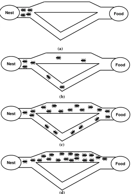
xc in the objective space...12 2.2 Main procedure of an evolutionary algorithm for single generation ...19 2.3 Above shows different kind of ranking schemes. (a) Goldberg’s nondominated sorting [25], (b) Fonseca’s ranking method [26], (c) Ranking scheme adopted in SPEA [27], and (d) Automatic accumulated ranking scheme proposed by [28]...22 2.4 Three diversity techniques proposed in [25,30,31] and used in various MOEAs. (a) In fitness sharing technique, fitness of an individual that share the same niche (dashed circles) with other individuals is reduced. (b) Grid approach is usually applied in archive for two purposes: diversity and archive maintenances. The grid regions represent a region. Individuals reside in crowded grid region have less chance to be selected. (c) In crowding distance scheme, distance of the individual, i and its two neighboring individuals (i.e. individuals of index i-1 and i+1) in each objective function are computed ... ...23 3.1 Ants’ foraging behavior in finding the shortest paths from their nest to the food source. (a) Ants are at the junction of the two paths that can lead to the food source from their nest. (b) The ants choose the path randomly. (c) Ants leave the pheromone trail while returning to their nest after find food. Shorter path (upper path) has higher pheromone concentration than longer path (lower path), which attracts more ants to choose the shorter path. (c) Eventually, All ants will end up using the shorter path...32 3.2 A boid’s neighborhood (in grey) and the triangular symbol (marked green) represents a boid [54,55]...35 3.3 The illustrations of the three steering behaviors of the boids. (The color in the illustrations are indicated as follow: the boid (in green and is attached with an red arrow), its neighborhood (in grey) and its local flockmates (in blue) [55].... ...36Figure Page 4.1 Position clipping criterion...45
4.2 Velocity clipping criterion ...46 4.3 Pseudocode of the generic PSO algorithm...47 4.4 Graphical representation of the three common neighborhood topology [75,76]:
(a) Global topology (gbest), (b) Ring topology (lbest), and (c) Star topology ...57 4.5 Graphical representation of the other neighborhood topology [75,76]: (a) Von Neumann, (b) Pyramid, and (c) Four Clusters ...57 5.1 Generic framework of MOPSO algorithm...68 5.2 Possible cases presented in [110]. Note that Ns denotes as nondominated solution; a no filled circle represents a new nondominated solution; and a filled or patterned circle represents a archive member ...73 5.3 Figure 5.3 Figures depicting the different strategies of selecting the global leaders. The arrows indicate the global leaders (filled circles) selected by the particles in the swarm (circles (no filled)) ...77 6.1 Pseudocode of DMOPSO ...93 6.2 Illustration of cell-based rank and density estimation scheme ...96 6.3 (a) Estimated objective space and divided cells, (b) initial rank value matrix of the given objective space, and (c) initial density value matrix of the given objective space [139,140] ...98 6.4 (a) Initial swarm population and the location of each particle, (b) rank value matrix of initial swarm population, and (c) density value matrix of initial swarm population [139,140] ...98 6.5 (a) New swarm population and the location of each particle, (b) rank value matrix of new swarm population, and (c) density value matrix of new swarm population [139,140]...98 6.6 Pseudocode of cell-based rank density estimation scheme [139, 140] ...99 6.7 (a) Current swarm population and the location of each particle, (b) rank value matrix of current swarm population, (c) density value matrix of current swarm population, and (d) example of “potential” particles, particles D and E ...101
Figure Page 6.8 Number of perturbation per particle, np versus iteration, t...102 6.9 The additional distance ∆d
( )
rb versus rb...103 6.10 (a) Selected particles (D and E) from Figure 6(d), (b) representation of Equation (9) in decision space, and (c) current swarm population and new added ones in objective space ...104 6.11 Pseudocode of population growing strategy ...105 6.12 (a) Current swarm population and the location of each particle, (b) rank matrix of current swarm population, and (c) R values for particles F and G ...106 6.13 (a) Current swarm population and the location of each particle, (b) density matrix of current swarm population, and (c) D values for particles F and G ... ...107 6.14 Pseudocode of population declining strategy ...109 6.15 (a) Two group leaders are grouped via clustering algorithm, (b) two group leaders in decision space are mapped to objective space, and (c) adaptive grid procedure is applied to local archive of G1 ...113 6.16 Pseudocode of adaptive local archives algorithm ...113 6.17 Sets H1, H2, and P are shown. By using the additive binary epsilon indicator, H1 strictly dominates H2 and H1 is strictly dominated by the true Pareto front. ...118 6.18 Box plot of hypervolume indicator (IH values) for all test functions (Startfrom top left) by algorithms 1-6 represented (in order): DMOPSO, OMOPSO, MOPSO, cMOPSO, sMOPSO, and NSPSO...120 6.19 Box plot based upon additive binary epsilon indicator (Iε+ values) on test
function ZDT1 (algorithms 1-5 are referred to as OMOPSO, MOPSO, cMOPSO, sMOPSO, and NSPSO, respectively)...122 6.20 Box plot based upon additive binary epsilon indicator (Iε+ values) on test
function ZDT2 (algorithms 1-5 are referred to as OMOPSO, MOPSO, cMOPSO, sMOPSO, and NSPSO, respectively)...123 6.21 Box plot based upon additive binary epsilon indicator (Iε+ values) on test
function ZDT3 (algorithms 1-5 are referred to as OMOPSO, MOPSO, cMOPSO, sMOPSO, and NSPSO, respectively)...123
Figure Page 6.22 Box plot based upon additive binary epsilon indicator (Iε+ values) on test
function ZDT4 (algorithms 1-5 are referred to as OMOPSO, MOPSO,
cMOPSO, sMOPSO, and NSPSO, respectively)...123
6.23 Box plot based upon additive binary epsilon indicator (Iε+ values) on test function ZDT6 (algorithms 1-5 are referred to as OMOPSO, MOPSO, cMOPSO, sMOPSO, and NSPSO, respectively)...124
6.24 Box plot based upon additive binary epsilon indicator (Iε+ values) on test function DTLZ2 (algorithms 1-5 are referred to as OMOPSO, MOPSO, cMOPSO, sMOPSO, and NSPSO, respectively)...124
6.25 Pareto fronts produced by (a) DMOPSO, (b) OMOPSO, (c) MOPSO, (d) cMOPSO, (e) sMOPSO, and (f) NSPSO on test function ZDT1 ...125
6.26 Pareto fronts produced by (a) DMOPSO, (b) OMOPSO, (c) MOPSO, (d) cMOPSO, (e) sMOPSO, and (f) NSPSO on test function ZDT2 ...125
6.27 Pareto fronts produced by (a) DMOPSO, (b) OMOPSO, (c) MOPSO, (d) cMOPSO, (e) sMOPSO, and (f) NSPSO on test function ZDT3 ...126
6.28 Pareto fronts produced by (a) DMOPSO, (b) OMOPSO, (c) MOPSO, (d) cMOPSO, (e) sMOPSO, and (f) NSPSO on test function ZDT4 ...126
6.29 Pareto fronts produced by (a) DMOPSO, (b) OMOPSO, (c) MOPSO, (d) cMOPSO, (e) sMOPSO, and (f) NSPSO on test function ZDT6 ...127
6.30 Pareto fronts produced by (a) DMOPSO, (b) OMOPSO, (c) MOPSO, (d) cMOPSO, (e) sMOPSO, and (f) NSPSO on test function DTLZ2...127
7.1 Pseudocode of DSMOPSO ...134
7.2 Pseudocode of update local best for the swarm leaders...138
7.3 Pseudocode of updating the particles...142
7.4 (a) Swarm leaders and their locations on the objective space, (b) rank matrix (Top) and density matrix (Bottom) of the swarm leaders, and (c) R and D values for swarm leaders E and F ...144
7.5 (a) Swarm leaders and their locations on the objective space, (b) rank matrix (Top) and density matrix (Bottom) of the swarm leaders, and (c) R, D, and rL values for swarm leaders E and F ...146
Figure Page 7.6 Block diagram depicts how an example Voronoi diagram of eight randomly
selected particles and xnew is generated...147
7.7 Pseudocode of generating a new swarm via Voronoi procedure ...148
7.8 Pseudocode of swarm growing strategy ...149
7.9 Pseudocode of swarm declining strategy...152
7.10 Illustration of objective space compression strategy (arrows in (b) signify the objective space is compressed) ...154
7.11 Illustration of objective space expansion strategy (arrows in (b) signify the objective space is compressed) ...154
7.12 Pseudocode of objective space compression and expansion strategy...158
7.13 Box plot of hypervolume indicator (IH values) for all test functions (Start from top left) by algorithms 1-4 represented (in order): DSMOPSO, DMOPSO, MOPSO, and cMOPSO...162
7.14 Box plot based upon multiplicative binary epsilon indicator (Iε+ values) all test functions (Start from top left) (algorithm A refer to DSMOPSO; algorithms 1-3 are referred to as DMOPSO, MOPSO, and cMOPSO, respectively) ...161-3
7.15 Pareto fronts produced by (a) DSMOPSO, (b) DMOPSO, (c) MOPSO, and (d) cMOPSO for ZDT1. The continuous line depicts the true Pareto front ...166
7.16 Pareto fronts produced by (a) DSMOPSO, (b) DMOPSO, (c) MOPSO, and (d) cMOPSO for ZDT2...166
7.17 Pareto fronts produced by (a) DSMOPSO, (b) DMOPSO, (c) MOPSO, and (d) cMOPSO for ZDT3...167
7.18 Pareto fronts produced by (a) DSMOPSO, (b) DMOPSO, (c) OMOPSO, and MOPSO for ZDT4 ...167
7.19 Pareto fronts produced by (a) DSMOPSO, (b) DMOPSO, (c) MOPSO, and (d) cMOPSO for ZDT6...168
7.20 Pareto fronts produced by (a) DSMOPSO, (b) DMOPSO, (c) MOPSO, and (d) cMOPSO for DTLZ2 ...168 7.21 Box plot of hypervolume indicator (IH values) for experiment with varying
Figure Page the swarm size. Note that 1-6 on x-axis represented (in order): swarm size of
2, 4, 6, 8, 12, and 20...172
7.22 Box plot of hypervolume indicator (IH values) for experiment with varying the grid scale (Ki). Note that 1-6 on x-axis represented (in order): Ki equals to 4, 5, 6, 7, 10, and 15...172
7.23 Box plot of hypervolume indicator (IH values) for experiment with varying the population size per cell (ppv). Note that 1-5 on x-axis represented (in order): ppv equal to 3, 5, 8, 12, and 25 ...173
7.24 Box plot of hypervolume indicator (IH values) for experiment with varying the δ parameter. Note that 1-7 on x-axis represented (in order): δ is equal to 0.1, 0.2, 0.3, 0.4, 0.5, 0.7, and 0.9...173
7.25 Box plot of hypervolume indicator (IH values) for experiment with varying the age threshold (Ath). Note that 1-6 on x-axis represented (in order): Ath is equal to 3, 4, 5, 6, 10, and 25 ...174
8.1 Illustration of bi-objective optimization problem (F
( )
x ). The feasible region is mapped to the solid segment. The shaded region represents the search space. The global optimum (black circle) is located beat the intersection of the Pareto front and the solid segment [155]...1858.2 Pseudocode of the proposed PSO algorithm to solve for COPs ...186
8.3 Pseudocode of updating the particles best archive ...188
8.4 Graph for percentage range to be reduced against T...195
8.5 Pseudocode of mutation operator applies to the swarm population ...195
8.6 Pseudocode of the proposed constrained MOPSO algorithm...198
8.7 Mutation rate (Pm) versus feasibility ratio of the particles’ personal best (rf)... ...203
8.8 Box plot of hypervolume indicator (IH values) for all test functions by algorithms 1-4 represented (in order): Proposed MOPSO, NSGA-II, GZHW, and WTY...214 8.9 Box plot of additive binary epsilon indicator (Iε+ values) for all test functions
Figure Page NSGA-II, GZHW, and WTY, respectively) ...216 8.10 Pareto fronts produced by the following algorithms a-d represented (in order): proposed MOPSO, NSGA-II, GZHW and WTY ...217
CHAPTER 1
INTRODUCTION
1.1 Motivation
In our daily lives, we encounter problems that demand us to search for the best possible solutions. These problems such as planning one’s day or monthly expenditure can be formulated as optimization problems. These problems are described by a mathematical model and objective function. An optimization problem with only one objective function is known as the single objective optimization problem (SOP). A best solution is usually obtained via either minimizing or maximizing a single objective function. However, many optimization problems encountered in the real world technical disciplines involve more than one objective. Usually, these objectives are conflicting with each other, e.g., maximizing return while minimizing risk measures in financial portfolio management. In this case, finding solutions by optimizing each objective independently is not the best way to do. If the optimum solution is found for one of the objectives it may lead to a compromise in achieving lower quality solutions by the other objectives. The optimization problems with more than one objective are referred to as multiobjective optimization problems (MOPs). An example of realistic MOPs is the aircraft design, in which the objectives comprise of fuel efficiency, payload, range, performance, speed and many other design considerations. Additionally, most real world MOPs are limited by a set of constraints. To optimize these so called constrained MOPs (CMOPs) are much
difficult since the set of optimum solutions (or the Pareto optimal set) are not only taken into consideration with trade-offs between the conflicting objectives but also must satisfy the constraints that impose upon the MOPs.
1.2 Objective
Various methods are available to tackle MOPs. The common choice is to employ the conventional methods (e.g., weighted sum method, goal programming, linear programming, min-max optimum, and etc.) or aggregating approach [1,2]. Most of these methods used to solve for MOPs follow the same design principle where all the objectives are combined together into one function by any means and optimize the new function as if it is a single objective optimization problem. These methods are not efficient in dealing with MOPs since they are designed to solve for one solution at a time instead of finding multiple solutions at once.
Heuristic methods, on the other hand, are favored in this case because they reduce the computational cost for high-dimensional optimization problems. Some of the heuristic methods, such as simulated annealing [3] and tabu search [4], face difficulty in solving MOPs, regardless of their stochastic nature, because they are not designed to find multiple solutions; while other heuristic methods, metaheuristics type, are better tools to solve MOPs. Evolutionary algorithms (EAs) are popular among the metaheuristics approaches [1,2,5-7]. They are population-based approach where multiple individuals search for a set of potential solutions in parallel and in a single run. Their design mechanisms reinforce their ability and flexibility in handling various types of problems with problem characteristics such as continuous, discontinuity, and multimodality.
Recently, a new metaheuristic design emerged from the field of swarm intelligence. This metaheuristic approach is called particle swarm optimization (PSO) [50]. It has shown great potential in solving single objective optimization problems [64-99] and has been modified necessarily to solve for MOPs [105-122]. Similar to EA, PSO also incorporates population-based approach and exhibits ability to deal with problems with different problem characteristics. The difference between PSOs and EAs is the fundamental mechanism design. EAs mimic the mechanism in biological evolution while the mechanism in PSO is inspired by the behavior of a bird flock. PSO presents two advantages over EA. PSO possesses faster convergence speed than EA and offers simplicity in implementation. Therefore, PSO is rapidly gaining attention among researchers. The advantages of PSO motivates this work in developing multiobjective optimization particle swarm optimization (MOPSO). The following discussion will relate to MOPSO unless specified otherwise.
Years of research has identified the desired attributes of a Pareto optimal set (solutions) that a multiobjective algorithm should achieve. A quality Pareto optimal set means the solutions are well extended, uniformly distributed, and near-optimal. Achieving such Pareto optimal set is challenging since it involves two compelling goals: to minimize the distance of the resulted solutions (Pareto optimal set or Pareto front) to the true Pareto set (or true Pareto front) and maximize the diversity of the resulted solutions [8]. Existing MOPSOs are designed with Pareto ranking schemes, archive maintenance strategies, and techniques to preserve the diversity, which guide the search towards a well extended, uniformly distributed, and near-optimal Pareto front.
However, to enhance the efficiency of a multiobjective optimization algorithm is not limited to develop ways to improve the convergence and techniques to promote diversity. In fact, the number of particles, i.e., swarm population size, to explore the search space in order to discover possible better solutions indirectly contributes to the efficiency improvement of an algorithm. The issue of determining an appropriate swarm population size is still at question. The easiest approach is to choose a larger population size since this would increase the chance for any MOPSOs to find the true Pareto front. A large population size, however, inevitably results in undesirable and high computational cost. Conversely, an insufficient swarm population size may result in premature convergence in MOPSO. Therefore, estimate an optimal population size requires many trial-and-error, especially for those MOPs with complicated landscape and unknown. One approach to address this disadvantage is to dynamically adjust the population size during the optimization process. Only few existing works under this research line are published, and they are all applied to MOEAs. Another approach to improve the performance of MOPSO is to employ the subpopulation concept. The reason is the swarm-like characteristic renders PSO aptness to adopt the subpopulation concept often referred to as multiple-swarm concept. Most publications in multiple swarms PSO are for single objective optimization and only a few apply this concept in multiobjective optimization. Therefore, the goal of this research is to study the dynamic population size and multiple-swarm concepts of the existing works, and develop state-of-the-art MOPSOs that fuse both elements to exploit possible improvement in efficiency and performance of existing MOPSOs.
The above discussion mainly focuses on multiobjective optimization algorithm to solve for unconstrained MOPs. Since in the real world application, many optimization problems involve a set of constraints (functions). Hence, an optimization tool must be able to handle these constraints, and also solve for the optimum solution for constrained optimization problems (COPs) or Pareto optimal set for constrained multiobjective optimization problems (CMOPs). Most EAs that are designed to solve for unconstrained MOPs lack a mechanism to handle constraints. In the past decade, many constraint handling techniques for EAs have been proposed. All these EAs are mainly aimed to solve for COPs and there are relatively less publications on MOEAs to solve for CMOPs. Since PSO is still a relatively new optimization algorithm, there is little work on applying PSO for COPs and applying MOPSO to solve for CMOPs. Thus, the second research goal is to design a MOPSO to solve for CMOPs. In order to develop the proposed MOPSO, it is essential to develop a PSO to handle constraint in COPs first and then extend the technique to design a MOPSO for CMOPs.
1.3 Contributions
The contributions of this thesis are summarized below.
• Develop a MOPSO that incorporates dynamic population and multiple swarm, in which the particles are grouped according to a user-defined number of swarms, for multiobjective optimization. This algorithm design involves dynamic swarm population strategy and adaptive local archives.
• Develop a framework for a MOPSO that dynamically adjust the number of swarms needed where under certain conditions new swarms may be added or
some existing swarms may be eliminated. Additional designs included in this algorithm are modified PSO update mechanism and objective space compression and expansion strategy.
• Develop a constrained PSO with design elements that exploit the key mechanisms to handle constraints as well as optimization of the objective function. The designs include updating personal best, maintaining feasible and infeasible global archive, adaptive acceleration constants in PSO, and mutation operators. These designs are also extended into a MOPSO to solve for CMOPs.
1.4 Outline of the Dissertation
This dissertation comprises of nine chapters and these chapters are organized as follows.
Chapter 2 provides the essential background of multiobjective optimization. Basic concepts of multiobjective optimization problem formulation and Pareto optimization are presented. Optimization methods and main topics related to multiobjective evolutionary algorithms, including test functions and performance metrics, are briefly reviewed.
Chapter 3 presents the background of the swarm intelligence field. The main objective is to understand swarm behavior, its unique benefits and the fundamental concept that render such behavior. Significant works of modeling the behavior of bird flock are reviewed since particle swarm optimization (PSO) is developed based on the principle of the social behavior of a bird flock.
In Chapter 4, history of particle swarm optimization (PSO) was discussed is presented. Then, the standard PSO equations and generic algorithm are introduced. Finally, we review the major modifications and advancements for improving the performance of original PSO. Related topics include the parameter settings, modification of the standard PSO equations, neighborhood topology, and incorporation of multiple-swarm concept into PSO.
Current works of multiobjective particle swarm optimizations (MOPSOs) that are relevant to this study are reviewed in Chapter 5. First, rationale of applying PSO for multiobjective optimization is discussed. Afterwards, a general framework of MOPSO along with the main themes related to the modification of MOPSOs is discussed.
Chapter 6 elaborates the first proposed MOPSO, namely dynamic multiobjective particle swarm optimization (DMOPSO). The chapter starts by discussing the role of population size when searching for potential solutions for a MOP. Two main concepts are incorporated: dynamic population and multiple swarms. Strategies to support the two concepts and to further improve the performance of the algorithm are detailed. Comparative study on the performance and computational cost of the DMOPSO against selected MOPSOs are analyzed.
Chapter 7 outlines the second MOPSO, i.e., dynamic multiple swarms in multiobjective particle swarm optimization (DSMOPSO). In this work, dynamic population concept is applied to regulate the number of swarms, which is different from DMOPSO in Chapter 6. Here, the number of particles in each swarm is fixed but the number of swarms is dynamically varied according to each contribution in searching for potential solutions during the search process. The development of the algorithm and key
design elements are described. Experiments to evaluate the performance and computational cost of the DSMOPSO are conducted. The chapter finishes with the sensitivity analysis and provides recommendation on the parameters settings.
In Chapter 8, a PSO and MOPSO are proposed to solve for constrained optimization problems. In this study, the multiobjective constraint handling formulation is applied. Design elements are proposed with the goal of guiding the particles towards feasible regions and leading them to the global optimum solution or the Pareto optimal set. Experiments are conducted on the benchmark functions to evaluate the performance of the proposed approaches.
Conclusions are discussed in Chapter 8. Summary of the main contributions of this thesis are reviewed. Limitations of the proposed works are identified and possible future research directions related to this study are recommended.
CHAPTER 2
MULTIOBJECTIVE OPTIMIZATION
Multiobjective optimization problems (MOPs) emerge in many fields. Difficulties arise when the MOPs involve multiple, conflicting objectives since the solution of the problems are more than one. Many conventional methods can be used to solve these MOPs but they are limited in certain aspects. Recent metaheuristics have brought the possibility of approaching MOPs in much simplistic and efficient ways. This chapter presents the basic concept of multiobjective optimization. In the following section, the background of selected optimization methods such as conventional algorithms, aggregating approaches and multiobjective evolutionary algorithms (MOEA) are elaborated. Finally, validation methodologies for MOEAs that are commonly used in many publications are presented.
2.1 Definition
Consider a minimization problem; the general form of the multiobjective optimization problem (MOPs) with kobjective functions is given as follows [1,2]:
( )
[
( ) ( )
, , ,( )
]
, minF x 1 x 2 x x x n F F Fk K = ℜ ∈ (2.1)subject to the m inequality constraints:
( )
0, j 1,2, ,m;gj x ≤ = K (2.2)
( )
0, j m 1, ,p;hj x = = + K (2.3)
and the ndecision variable bounds:
. , , 2 , 1 , i n x x xiL ≤ i ≤ Ui = K (2.4) where x=
[
x1,x2,K,xn]
∈ℜn. (2.5)The function Fi is known as the objective function or fitness function, and Fi
( )
x is called the fitness or fitness value of Fi. x represents a decision vector of ndecision variables, where each decision variable is bounded by a lowerxiL, and an upperxiU bound. The n variable bounds constitute a decision space or search space, S⊆ℜn, and the kobjective functions constitute a objective space, Z. Decision vectors that minimize( )
xF are also referred as solutions. gj
( )
x represents the jth inequality constraint while( )
xj
h represents the jth equality constraint. The inequality constraints that are equal to zero, i.e., gj
( )
x* =0, at the global optimum (x*) of a given problem are called active constraints. The feasible region (F ⊆S) is defined by satisfying all constraints (Equations (2.2)-(2.4)). A solution in the feasible region (x∈F) is called a feasible solution, otherwise it is considered an infeasible solution. All the solutions that lie on the feasible region is called the feasible set,Φ. Equation 2.1 presents the case of minimizing all the objective functions. By duality principles, any objective function can be converted from minimization form to maximization form or vice versa, which is given below [5]:( )
x(
i( )
x)
i F
F =min −
max (2.5)
2.1.1 Pareto Optimization
For single objective optimization, the aim is to search for the best possible solution available, or the global optimum [6]. However, for MOPs, provided that the objectives functions are conflicting to each other, there is not just a single optimum solution but a set of optimal solutions. To obtain the set of optimum solutions, the concepts of Pareto dominance and Pareto optimality are adopted. The following discussion presents the key definitions that related to the concepts [1,2,7]:
Definition 2.1 (Concept of Pareto Dominance)
Consider a minimization problem, a decision vector xa is said to dominate another decision vector xb, denoted by xa pxb, iff
1. Fi
( )
xa ≤Fi( )
xb for all i=1,2,K,k and2. Fj
( )
xa <Fj( )
xb for at least one j∈(
1,2,K,k)
Definition 2.2 (Nondominated Set)
Let Ρ represent the set of decision vectors in the feasible region, Ρ⊆Φ, the nondominated set are those decision vectors in Ρ that are not dominated by any members of the set Ρ, (i.e. all individuals in the nondominated set are feasible).
Definition 2.3 (Pareto Optimal Set)
A feasible decision vector x* is Pareto optimal if there exist no feasible decision vector xi for which F
( )
xi dominates F( )
x* . The collection of such decision vectors(a) (b)
Figure 2.1 The decision vectors x , a x , and b x in the feasible region in decision space and their c
corresponding fitness F
( )
xa , F( )
xb , and F( )
xc in the objective space.that are Pareto optimal is known as the Pareto optimal set. This means that each solution in this set holds equal importance and is a good compromise among the trade-off objectives. The resulted tradeoff curve in the objective space that obtained from Pareto optimal set is called the Pareto front.
2.1.2 Example
Consider a minimization problem; Figure 2.1 presents a representation of the feasible region in the decision space and the corresponding feasible objective space. Referring to Figure 2.1, the decision vectors xa, xb, and xc in the decision space are mapped to the three fitness, i.e., F
( )
xa , F( )
xb , and F( )
xc respectively in the objective space. Observe Figure 2.1(b), the solution xbdominates solution xa, since the objective( )
b F( )
aF1 x < 1 x and F2
( )
xb < F2( )
xa , which satisfies the two conditions of Definition 2.1. Apply the same definition, solution xc is also found to dominate solution xa. For solutions xb and xc, both do not dominate each other because Condition 2 of Definition1 x 2 x 1 F 2 F
Pareto optimal set
a x c x b x F
( )
xb F( )
xa( )
xc FDecision space Objective space
Feasible region 1 x 2 x 1 F 2 F
Pareto optimal set
a x c x b x F
( )
xb F( )
xa( )
xc FDecision space Objective space
2.1 is violated. In addition, solutions xband xcare not dominated by another solution; hence according to Definition 2.2, xband xc belong to the nondominated set. The Pareto optimal set, also the Pareto front or the tradeoff curve, is illustrated in Figure 2.1(b).
2.2 Optimization Methods
After the invention of the computer, research in optimization field been active ever since. Various optimization methods are designed and created to solve for optimization problems. There are two main classes: the conventional methods and the modern heuristics.
Table 2.1 Examples of optimization methods under the two main classes.
Conventional Methods Modern Heuristics
Branch and Bound Tabu Search
Dynamic Programming Simulated Annealing Linear Programming Differential Algorithm
Min-max Optimum Evolutionary Algorithms
Newton’s Method Cultural Algorithm
Divide and Conquer Particle Swarm Optimization Goal Programming
etc…
Ant Colony Optimization etc…
Conventional methods adopt the deterministic approach. During the optimization process, any solutions found are assumed to be exact and the computation for next set of solutions completely depends on the previous solutions found. That’s why conventional methods are also known as deterministic optimization methods. In addition, these methods involve certain assumptions about the formulation of the objective functions and constraint functions. Conventional methods include algorithms such as branch and bound, dynamic programming, linear programming, min-max optimum, and those listed in Table 2.1. There is a subclass under modern heuristics, which is called the stochastic based
methods. The algorithms that are categorized as stochastic based methods include simulated annealing, evolutionary algorithms, differential algorithm, cultural algorithm, and particle swarm optimization. These algorithms possess the stochastic nature while searching for possible solutions for a problem. In the following, elaboration on conventional algorithms, aggregating approach, and evolutionary algorithms are presented.
2.2.1 Conventional Algorithms
Conventional algorithms or classical methods have been around for at least four decades [1]. They possess the deterministic and predictable behavior, in which the techniques are designed to find the same solution if the same input sample and stopping criteria are applies. The search process will be much efficient and quicker if the input is located within some defined finite search space provided that the search space is not overly large. Publications have shown the success of employing these algorithms in solving a wide variety of problems [9-11], but not for problems that are high dimensional, multi-modal or NP-complete problems.
Conventional algorithm can solve MOPs. These techniques used for handling MOPs share a similar spirit, which is to convert the MOPs into a single objective optimization problem and find a preferred Pareto optimal solution [1]. Refer to the classification of algorithms given by Hwang and Masud [12], these algorithms are under the class of priori preference [7]. The best represented algorithms include weighted-sum method, the Goal programming method, and the min-max optimum.
Weighted-sum method [1,2,7,13] – The aggregating function is derived by pre-multiplied the multiple objectives functions with the corresponding predefined weights. Mathematically, the aggregating function is in the form:
( )
∑
( )
= = k i i iF w F 1 x x , (2.7)where wi are the weighting coefficients, within the range of
[ ]
0,1 . These weighting coefficients represent the relative significances of the objective functions. To maintain the same order of scale among the objective functions, the objective functions are normalized first before applying Equation (2.7). In addition, the weighting coefficients are chosen such that the sum of these weighting coefficients is one, i.e.,∑
= = k i i w 1 1, (2.8)This method has its disadvantages. It is sensitive to the weighting coefficients chosen heuristically, so prior knowledge is needed to predetermine the weights. In addition, it fails to find solutions that locate on the concave portions of the Pareto front [7].
Goal Programming Method – This method is introduced by Charnes and Cooper [14,15] in 1960s and due to its simplicity, is has applied to various fields [16,17]. The main idea is to find solutions that attain a set of predefined goals for the corresponding objective functions [1]. The general steps to find solutions by using this method are given below:
Step 1: For MOPs with kobjective functions, pre-specify a set goal, ti, where
k i=1,2,K,
Step 2: Setup k generic constraint equations based on the given goals, types of goal criteria, and the corresponding kobjective functions. For example, the constraint equations for four different types of goal criteria are given as follows [1]:
1. Less-than-equal-to,F
( )
x ≤t:Generic constraint equation: F
( )
x − p≤t; (2.9) 2. Greater-than-equal-to, F( )
x ≥tGeneric constraint equation: F
( )
x +n≥t; (2.10) 3. Equal-to, F( )
x =tGeneric constraint equation: F
( )
x − p+n=t; (2.11) 4. Range, F( )
x ∈[
tL,tU]
Generic constraint equation: F
( )
x − p≤tL and F( )
x +n≥tU; (2.12) The two new variable(s) appeared in Equations (2.9) to (2.12), i.e., pand n, are called the deviational variables. The aim of adding the variable(s) is to measure the difference between the goal and the achieved levels of the corresponding objective function. Detail on how Equations (2.9) to (2.12) are obtained is given in [1,14,15].Step 3: Once the constraint equations are set, optimization technique is applied to optimize all the deviational variables as a weighed sum single objective function that subject to k constraint equations (given in Step 2). If it is a minimization problem, then all the deviational variables are to be minimized. There are many techniques available [17,18]. Among them, the common ones are the weighted goal programming (WGP) and the lexicographic goal programming (LGP).
The disadvantage of this method is need of prior knowledge to set the predefined goals for their corresponding objective functions.
Min-max Optimum – This approach is one of the techniques used in the field of game theory. Due to its design to deal with conflicting situation, it has been employed in solving the MOPs [19]. In this method, the set of solutions found will have the minimum deviation between the solutions and the individual objective function. The “min-max” criteria are used to compare relative deviation of the current best points and the individual objective function at every iterations until the set of solution is found. Detailed procedure of this method can be found in [19]. This method is capable of discovering all optimum solutions for a given the MOPs regardless if the problem is convex or nonconvex [7]. The disadvantage of min-max optimum is applied to each of the objective functions individually.
In solving the MOPs, the goal is to find the Pareto optimal set. In this case, conventional algorithm can only find one solution in one run with a fixed parameter setting. Note that a single run means that an algorithm continues its process to search for solutions until it meets the stopping criteria. Hence, to find the Pareto optimal set, multiple runs with different parameter settings for every individual objective function are required. In addition, some of these algorithms such as weighted-sum method may require prior knowledge of the problem to predetermine some of the fixed parameters; while some algorithms have difficulty in solving MOPs that have convex Pareto front [2].
2.2.2 Aggregating Approaches
In aggregating approaches, techniques are employed to combine multiple objective functions into a single objective function using either addition, multiplication, or any other combination of arithmetical operations [2]. The techniques are also known as aggregating functions and can be either linear or nonlinear. A simple example of an aggregating approach is the weighted-sum method. In general, many have known that aggregating function poses a well-known limitation, which is the difficulty in finding the concave portion of the Pareto front. However, this limitation does not necessarily hold if a nonlinear aggregating function is adopted [6]. Hence, the limitations of the aggregating approach depend on the technique employed. Although an aggregating approach may be able to find an optimum solution at each run, many runs are needed to obtain the complete optimal Pareto front for a given MOPs.
2.2.3 Multiobjective Evolutionary Algorithms (MOEAs)
Since the groundbreaking work of computer simulation of evolution in 1954 [20], along with various researchers’ contributions in developing new computer simulations that merge evolution theory with computational methods, the new field of evolutionary computation has arisen. In evolutionary computation, the algorithms are population based. The population undergoes processes that iteratively guide it to achieve the desired goal. The processes can be inspired by concepts that are different from the mathematical or computer field, such as biological mechanisms of evolution or social behaviors. Among the computational techniques in evolutionary computation, evolutionary algorithms (EAs) adopted mechanism that inspired by the principle of biological
evolution [21]. EAs comprise of some well-known techniques [21-23], for instance, genetic algorithm, evolutionary programming, evolutionary strategy, and genetic programming where each employs the mechanisms of evolution yet differ in implementation.
The main disadvantage of using conventional algorithms and other mathematical programming techniques to solve MOPs are most of them are designed to solve for specific problems only and they find only one, at most, optimum solution in a single run, multiple runs are necessary to complete the Pareto front. EAs can overcome this disadvantage. Research in developing evolutionary algorithms to solve MOPs have
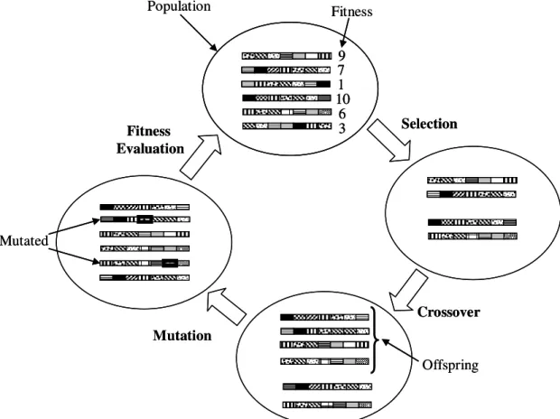
Figure 2.2 Main procedure of an evolutionary algorithm for single generation.
9 10 7 1 6 3 Population Fitness Fitness Evaluation Selection Mutation Crossover Offspring Mutated 9 10 7 1 6 3 9 10 7 1 6 3 Population Fitness Fitness Evaluation Selection Mutation Crossover Offspring Mutated
gained much attention for over 20 years and these algorithms are called multiobjective evolutionary algorithm (MOEA).
2.2.3.1 General Concept
The main idea of evolutionary algorithm (EA) is to model the fundamental mechanisms of evolution and utilizes evolution concept to perform optimization process. Five main mechanisms mimicked and incorporated into an EA are reproduction, natural selection, survival of the fittest, crossover, and mutation. In EA, a candidate solution, denoted as an individual, is encoded as genes in the chromosomes. A set of candidate solutions are referred to as population. During a series of iterations, or called generations, the individuals are evaluated to determine their fitness value. Based on their fitness value, those that are considered the fitter ones are selected by the selection operator because they have higher probabilities to produce “fitter” individuals (offsprings). Hence, two of the selected individuals that are randomly chosen are denoted as parents. Next, crossover operation and occasionally followed by mutation operator are applied to the parents to produce new individuals or offsprings. This reproduction process is applied to all the selected individuals. Figure 2.2 illustrates the main procedure of an evolutionary algorithm for single generation.
2.2.3.2 A Brief Tour of MOEAs
Various designs of MOEAs have been developed since the 1980s. The pioneering work of MOEA is called vector evaluated genetic algorithm (VEGA), designed by Shaffer [24]. At each generation, the whole population is divided into subpopulations of equal size. The number of subpopulations depends on the number of objective functions
in a MOPs. These subpopulations are combined and shuffled together. Crossover and mutation operators are applied to the shuffled population to obtain new population. Advantage of VEGA is its simplicity to implement and its disadvantage is the tendency to generate good solutions for one of the objective but not for all of the objectives because the selection operator would incline to select a subpopulation with better fitness values than the others.
The mark of significant contribution to MOEAs development is after David E. Goldberg’s proposal of the concept of Pareto optimality [25]. His idea is to assign ranks to the individuals based on their relative Pareto dominance. Hence, the selection process is based on these rank values of the individuals. Selection pressure is imposed to guide the population towards the direction of the Pareto front. Goldberg’s ranking scheme is known as the nondominated sorting (Figure 2.3 (a)) and have sparked the interest of designing Pareto based MOEAs. Several MOEAs have adopted his scheme. Among those are niched Pareto genetic algorithm (NPGA) [186] and nondominated sorting genetic algorithm (NSGA)[187]. Improved versions of Goldberg’s ranking scheme are introduced in several publications. Figure 2.3 shows different Pareto ranking schemes of [25-28]. There are Fonseca’s Pareto ranking scheme where the rank of an individual is corresponding to the number of other individuals that dominate it [26] (in Figure 2.3 (b)); ranking scheme proposed by SPEA [27] (refer to Figure 2.3 (c)) where fitness assignment strategy is modified to determine the “strength” of each individual, instead of rank; and automatic accumulated ranking scheme by [28] where individual’s rank is corresponding to the accumulated rank of those individual that dominate it, as shown in Figure 2.3(d).
Second significant advancement in the MOEA research area is the introduction of elitism or archiving concept. Purpose of archive is to store the good solutions (i.e., nondominated solutions) found thus far from the search process. Issue of adopting archiving is what strategy to maintain the archive. The most popular of incorporation of elitism concept is introduced by Zitzler and Thiele [27]. They adopted two populations in their proposed MOEA, called strength Pareto evolutionary algorithm (SPEA). One population contains the individuals that search for solutions while the other is an external population or archive that stores limited nondominated soutions found at every generation. To maintain the archive, strength values are assigned to the solutions in the archive. These strength values will play a role in computing fitness of the current
(a) (b)
(c) (d)
Figure 2.3 Above shows different kind of ranking schemes. (a) Goldberg’s nondominated sorting [25], (b) Fonseca’s ranking method [26], (c) Ranking scheme adopted in SPEA [27], and (d)
Automatic accumulated ranking scheme proposed by [28]. 1 F 2 F 1 F 2 F 1 1 1 1 2 2 2 3 1 1 1 1 3 2 2 4 4 3 1 F 2 F 1 F 2 F 1 F 2 F 1 F 2 F 1 1 1 1 2 2 2 3 1 1 1 1 3 2 2 4 4 3 1 F 2 F 6 2 6 4 6 2 0 6 12 6 12 6 10 6 12 6 8 1 F 2 F 1 1 1 1 3 2 8 5 2 1 F 2 F 6 2 6 4 6 2 0 6 12 6 12 6 10 6 12 6 8 1 F 2 F 1 F 2 F 1 1 1 1 3 2 8 5 2
(a) Fitness sharing (b) Grid (c) Crowding distance
Figure 2.4 Three diversity techniques proposed in [25,30,31] and used in various MOEAs. (a) In fitness sharing technique, fitness of an individual that share the same niche (dashed circles) with other individuals is reduced. (b) Grid approach is usually applied in archive for two purposes:
diversity and archive maintenances. The grid regions represent a region. Individuals reside in crowded grid region have less chance to be selected. (c) In crowding distance scheme, distance of the
individual, i and its two neighboring individuals (i.e. individuals of index i-1 and i+1) in each objective function are computed.
population, which indirectly place preference to individuals that are least dominated and those that located in less populated region in the objective space. Clustering algorithm is applied to maintain the archive size and to promote diversity. Zitzler and Thiele’s [27] elitism concept brought interest to many researchers to incorporate this concept to their new MOEAs. Significant work with new elitism strategies include SPEA2 [29], PAES [30], NSGA-II [31], PESA [32], and micro-GA [33].
Diversity maintenance is essential to prevent the “genetic drift” effect that causes the loss of diversity in the population. A number of works have proposed various techniques to encourage diversity. Among them, the established diversity techniques include fitness sharing [25], grid [30], and crowding distance [31], as illustrated in Figure 2.4. Please note the numbers shown next to individuals are the assigned rank values according to each specific design.
1 F 2 F 1 F 2 F 1 F 2 F i-1 i+1 i cuboid 1 F 2 F 1 F 2 F 1 F 2 F 1 F 2 F 1 F 2 F i-1 i+1 i cuboid 1 F 2 F i-1 i+1 i cuboid
2.3 Test Functions
It is a common practice that after a MOEA is proposed, its performance is validated from the standard simulated testing process. Applying the new algorithm to a set of test functions or benchmark problems is part of the simulated testing process to show the efficiency in solving the problems. Usually, the benchmark problems are selected from a variety of available standard test functions, which they all have their own representations, difficulties and properties (i.e., multifrontality, discontinuity, and convexity in the Pareto optimal front [2]).
The earlier test functions designs for MOEA are simpler and often with two objectives [34-37]. In the last several years, several researchers have developed sets of test functions that have become the standard benchmark functions in many MOEA research publications [38-40]. Introduction of toolkits to design test functions facilitates constructing desired test suites [38-42]. Recall that the two key tasks that a MOEA should accomplish are to converge towards the optimal Pareto front and to maintain the diverse distribution of the optimal Pareto front solutions. Hence, in test problem design, these two tasks are the criteria to determine the difficulty level of the test problem. In [38], method to construct a test function is based on two basic functions, i.e. function
hand function g. Consider a two objectives test function, the first objective, F1
( )
x , influences the level of distribution of the Pareto optimal solutions, while the second objective, F2( )
x , is designed from the combinations of the two basic functions and F1( )
x . Function h designs the shape of the Pareto front in the objective space and functionZitzler et al. [39] and [40] produced standard and practical benchmark problems that are currently used for performance testing of MOEAs in many publications.
Another work by Okade et al. steered away from the method proposed by [38] and proposed their own method that can construct various benchmark functions with arbitrary, customized Pareto front in objective and in decision spaces [41]. They also proposed a distribution indicator to measure the difficulty of the benchmark functions based on the mapping from the decision space to the objective space. In [42], the limitations of the existing benchmark functions are analyzed. They recommended that a test suite should contain test problems with a wide range of possible features [42]. In addition, a toolkit (i.e. WFG Toolkit) to construct unconstrained test problems is proposed to provide control and flexibility to the users to design test suites that meet the desired features. Using WFG Toolkit, the authors designed a test suite that consists of test problems with various features. This new test suite may be considered complete at this time. Once this new test suite gains popularity, it would become one of those standard test functions in the MOEA field. As indicated in [6], future test functions are expected to be more complex and cover wider range of aspects and features that are closer to the real-world problems.
2.4 Performance Metrics
Metrics are applied to assess the performance of a MOEA after it finds the optimal Pareto front for a chosen test function. Performance metrics for MOEA are different from algorithms that deal with SOPs. Since the optimal solution for MOPs is a set of solutions, the designed metrics have to measure multiple solutions. In addition,

![Figure 2.3 Above shows different kind of ranking schemes. (a) Goldberg’s nondominated sorting [25], (b) Fonseca’s ranking method [26], (c) Ranking scheme adopted in SPEA [27], and (d)](https://thumb-us.123doks.com/thumbv2/123dok_us/10121126.2912706/40.918.199.765.521.991/figure-different-ranking-schemes-goldberg-nondominated-fonseca-ranking.webp)

![Figure 4.4 Graphical representation of the three common neighborhood topology [75,76]: (a) Global topology ( gbest ), (b) Ring topology ( lbest ), and (c) Star topology](https://thumb-us.123doks.com/thumbv2/123dok_us/10121126.2912706/75.918.208.758.580.765/figure-graphical-representation-neighborhood-topology-topology-topology-topology.webp)

![Figure 5.2 Possible cases presented in [110]. Note that Ns denotes as nondominated solution; a no filled circle represents a new nondominated solution; and a filled or patterned circle represents a](https://thumb-us.123doks.com/thumbv2/123dok_us/10121126.2912706/91.918.196.751.98.696/possible-presented-nondominated-solution-represents-nondominated-patterned-represents.webp)