EFFICIENT DATA RECONFIGURATION FOR TODAY’S CLOUD SYSTEMS
BY
MAINAK GHOSH
DISSERTATION
Submitted in partial fulfillment of the requirements for the degree of Doctor of Philosophy in Computer Science
in the Graduate College of the
University of Illinois at Urbana-Champaign, 2018
Urbana, Illinois Doctoral Committee:
Professor Indranil Gupta, Chair Professor Nitin Vaidya
Professor Luke Olson
Abstract
Performance of big data systems largely relies on efficient data reconfiguration techniques. Data reconfiguration operations deal with changing configuration parameters that affect data layout in a system. They could be user-initiated like changing shard key, block size in NoSQL databases, or system-initiated like changing replication in distributed interactive analytics engine. Current data reconfiguration schemes are heuristics at best and often do not scale well as data volume grows. As a result, system performance suffers.
In this thesis, we show thatdata reconfiguration mechanisms can be done in the background by using new optimal or near-optimal algorithms coupling them with performant system de-signs. We explore four different data reconfiguration operations affecting three popular types of systems – storage, real-time analytics and batch analytics. In NoSQL databases (storage), we explore new strategies for changing table-level configuration and for compaction as they improve read/write latencies. In distributed interactive analytics engines, a good replication algorithm can save costs by judiciously using memory that is sufficient to provide the high-est throughput and low latency for queries. Finally, in batch processing systems, we explore prefetching and caching strategies that can improve the number of production jobs meeting their SLOs. All these operations happen in the background without affecting the fast path. Our contributions in each of the problems are two-fold – 1) we model the problem and design algorithms inspired from well-known theoretical abstractions, 2) we design and build a system on top of popular open source systems used in companies today. Finally, using real-life workloads, we evaluate the efficacy of our solutions. Morphus and Parqua provide several 9s of availability while changing table level configuration parameters in databases. By halving memory usage in distributed interactive analytics engine, Getafix reduces cost of deploying the system by 10 million dollars annually and improves query throughput. We are the first to model the problem of compaction and provide formal bounds on their runtime. Finally, NetCachier helps 30% more production jobs to meet their SLOs compared to existing state-of-the-art.
Acknowledgments
At the very start, I would like to thank my advisor, Professor Indranil Gupta (Indy). Over the years, he has advised me on challenging problems to work on, books to read, food to try, travel destinations. The fact that I could talk to him on a wide variety of topics (work and non-work) helped me a lot in settling down in this place away from home. Thanks Indy for guiding me through this long journey.
I would also like to thank my thesis committee members, Professor Nitin Vaidya, Professor Luke Olson and Professor Aaron Elmore. Your feedback has been invaluable and has helped in improving the thesis. Thanks to all the funding agencies who have supported my work. I would also like to thank the department for giving me this opportunity to pursue Ph.D. in this great institute. Thanks to all the professors whose courses I had the privilege to take and learn from. Thanks to all the admins for your tireless work to ensure a smooth graduate life here for me.
I have actively collaborated with researchers from industry and academia in my projects. I would like to take this opportunity to thank, Wenting Wang, Gopalakrishna Holla, Yosub Shin, Ashwini Raina, Le Xu, Xiaoyao Qian, Himanshu Gupta, Shalmoli Gupta, Nirman Kumar, Professor Chandra Chekuri, Professor Aaron Elmore, Virajith Jalaparti, Chris Dou-glas, Ashvin Agrawal, Avrilia Floratou, Ishai Menache, Joseph (Seffi) Naor, Sriram Rao, Kaushik Rajan. I cherish the stimulating discussions we had on the different projects we worked together. It was a learning experience and has helped me immensely in not only understanding the problem at hand but also appreciate the big picture.
I have had the opportunity to make some wonderful friends in Urbana-Champaign. I have had the pleasure of your company in restaurants, movies, travels, random discussions, cele-brations. Thank you Sourabh, Ankita, Swarnali, Srijan, Sreeradha, Debapriya, Sangeetha, Subhro, Faria, Le, Muntasir. I greatly value our time spent. A big shout out to the vibrant communities I got to engage with – Distributed Protocols Research Group (DPRG), Bengali Student’s Association (BSA), East Central Illinois Bengali Association (ECIBA) and ASHA for Education.
Next, I would like to thank my mother, Kakali Ghosh and my father, Mrinmoy Kumar Ghosh. You have cheered at all my milestones and helped me get up when I was feeling low. Thank you for teaching me to value relationships, family, friends, objects, and life itself. I try my best to follow your footsteps and be the person that you wanted me to be. At different points in my growing up years, you chose to let go of smaller pleasures in your life to help me succeed in my career and life. Pursuing a Ph.D. in the U.S.A. was one such moment
when you let me go despite realizing how far I would have to move. I am sorry that you had to sacrifice so much. I am not sure if I can ever make it up to you. Thank you for being the best parents.
Finally, I would like to thank my partner, my confidant, my best friend, Shalmoli. I am deeply indebted to the University for bringing us together. Shalmoli, you are the most amazing person I have met. In the last few years, you have made the highs more special and lows more bearable. Your enthusiasm and exuberance on different facets of life inspires me. Thanks for being the special person of my life.
Table of Contents Chapter 1 Introduction . . . 1 1.1 Background . . . 1 1.2 Challenges . . . 3 1.3 Contributions . . . 5 1.4 Roadmap . . . 6
Chapter 2 Morphus: Supporting Online Reconfigurations in Sharded NoSQL Systems 8 2.1 Introduction . . . 8
2.2 System Design . . . 10
2.3 Algorithms for Efficient Shard Key Reconfigurations . . . 15
2.4 Network-Awareness . . . 18
2.5 Evaluation . . . 20
2.6 Related Work . . . 30
2.7 Summary . . . 31
Chapter 3 Parqua: Online Reconfigurations in Virtual Ring-Based NoSQL Systems 32 3.1 Introduction . . . 32
3.2 System Model & Background . . . 34
3.3 System Design and Implementation . . . 35
3.4 Experimental Evaluation . . . 38
3.5 Summary . . . 50
Chapter 4 Popular is Cheaper: Curtailing Memory Costs in Interactive Analytics Engines . . . 51
4.1 Introduction . . . 51
4.2 Background . . . 54
4.3 Static Version of Segment Replication Problem . . . 56
4.4 Getafix: System Design . . . 62
4.5 Evaluation . . . 68
4.6 Discussion . . . 77
4.7 Related Work . . . 78
4.8 Summary . . . 79
Chapter 5 Fast Compaction Algorithms for NoSQL Databases . . . 80
5.1 Introduction . . . 80
5.2 Problem Definition . . . 82
5.3 Greedy Heuristics for BinaryMerging . . . 84
5.4 Simulation Results . . . 90
Chapter 6 Joint Network and Cache Management for Tiered Architectures . . . 96 6.1 Introduction . . . 96 6.2 Motivation . . . 99 6.3 System Architecture . . . 102 6.4 Implementation . . . 105 6.5 Evaluation . . . 108 6.6 Related Work . . . 114 6.7 Conclusion . . . 115
Chapter 7 Conclusion and Future Work . . . 116
Chapter 1: Introduction
1.1 BACKGROUND
Data driven business intelligence (BI) has seen a steady adoption [1] across multiple sectors (telecommunication, financial services, healthcare, technology, etc) and among corporations, governments, non-profits, alike. Early BI tools were primitive and often required manual sifting through multiple long spreadsheets. One of the key challenges was lack of software and hardware capable of handling large volumes of data. The last decade has seen tremendous growth in both areas which has enabled organization to make business critical decisions in real time. Today, big data has impacted gene sequencing for faster drug discovery, making smart energy efficient homes, self driving cars, solving food wastage, help farming with precision tools, etc.
Tools for data driven business intelligence can be broadly classified into two categories – storage and computation. While the former is required to store data generated in a company, the latter is used for running analysis on the stored data. Computation systems are designed to be massively parallel, fault tolerant, handle stragglers, etc. Storage systems provide high availability, fault tolerance, consistency.
Google’s Mapreduce [2] was one of the early computation systems that has inspired today’s systems like Hadoop [3] and Spark [4]. These systems are popularly called batch processing systems. They handle large amount of data at rest and can run analytics jobs which can span from few hours to few days. One of the first open-source batch processing systems, Hadoop captures 21% [5] of the total analytics markets with 14K companies using and in some cases actively contributing to the project. Spark is an academic project from UC Berkeley which has henceforth been commercialized and has seen steady adoption in internet companies like Facebook, Twitter, etc.
Along with Mapreduce, Google also built storage systems like Bigtable [6] and Google File System [7] which stored petabytes of data across many servers. Later, GFS inspired open source development of HDFS [8]. Similarly, Bigtable and Dynamo [9], a storage system from Amazon around the same time, inspired some of the present day open source NoSQL databases like HBase [8], Cassandra [10], MongoDB [11] etc. HDFS is the de facto stan-dard for companies storage needs and works as the storage substrate for the popular batch processing system Hadoop. NoSQL databases have been adopted in internet companies like Facebook, Google, telecommunication companies like Verizon, retail chains like Walmart, Amazon, etc.
studies have also shown that lack of realtime responses in ecommerce sites, can lead to re-duced profitability anywhere between 25% to 125% [12]. Hadoop and Spark do not satisfy these requirements as they were not built for response latencies in the order of seconds. The real time analytics space has developed under two verticals – streaming analytics and distributed OLAP. Systems like Samza [13], Heron [14] fall into the streaming space while Apache Kylin [15], SQL Server [16] are some examples of OLAP systems. In the intersec-tion lies distributed interactive analytics engine. Some popular systems in this space are Druid [17], Presto [18]. This area is expected to grow to 13.7 billion dollars by 2021 [19]. Companies currently maintain separate pipelines for batch and realtime analytics.
In the next decade, we expect data volumes to reach hundreds of zettabytes [20, 21]. Simul-taneously, companies will continue to add newer pipelines to satisfy specialized application use-cases. Machine learning systems [22] are an example. Often many of these pipelines end up sharing the same data. Data Lakes [23] have seen adoption because they allow easy data sharing as well as independent scale out capabilities.
One of the major challenges in storage in this upcoming era is managing data reconfigura-tion operareconfigura-tions at scale. Reconfigurareconfigura-tion operareconfigura-tions handle how data is laid out in a cluster. For example, shard key in a NoSQL database is a popular configuration that defines how to partition data in a table. Changing shard key is a reconfiguration operation that involves repartitioning and reassigning data to different physical machines. Reconfiguration opera-tions are necessary in a system to improve performance. For example, changing shard key helps in improving read/write latency in NoSQL databases. They can be user-initiated like a sys-admin in a company or system initiated. They are commonly used in both compute and storage systems. Since reconfiguration operations change properties associated with data, these operations are I/O bound, often saturating network or disk.
Type of
System Reconfiguration Metric AffectedPerformance Applicable to Chapter
Storage Table-level Configuration Change Read/Write Latency NoSQL Databases like MongoDB and Cassadra Chapter 2 Chapter 3 Compaction Read Latency
NoSQL Databases
like Cassandra Chapter 5 Real Time
Analytics Replication Query Throughput
Distributed Interactive Analytics Engine
like Druid Chapter 4 Batch
Analytics
Prefetching
and Caching Meeting Job SLOs System like HDFSDistributed File Chapter 6 Table 1.1: Reconfiguration Operations Explored in this Thesis. We picked operations that straddle different systems from storage to real-time analytics to batch processing system. All of them affect a key system performance metric.
Table 1.1 lists four popular data reconfiguration operations commonly seen in storage and computation systems of today and the performance metrics they affect. We observe that current state-of-the-art solutions for these operations are heuristic at best and often involve manual work from a sys-admin. In our thesis, we claim data reconfiguration mechanisms can be done in the background by using new optimal or near-optimal algorithms coupled with performant system designs..
For each of the reconfiguration operations mentioned in Table 1.1, we make the following two-fold contributions – 1) we model the problem and design algorithms inspired from well-known theoretical abstractions, 2) we design and build a system on top of popular open source systems used in companies today. We have the following goals for system design – 1) reconfiguration should happen in the background without affecting the normal query path, 2) minimizing total data transfer required, 3) minimizing impact on query latency. Finally, using real-life workloads, we evaluate the efficacy of our solutions. Our evaluation results vindicate our thesis and shows that one can build efficient data reconfiguration strategies by merging theory with practical design principles.
In Section 1.2, we describe the challenges involved in each of the reconfiguration operation listed in Table 1.1. In Section 1.3, we outline the contributions we made to solve these challenges.
1.2 CHALLENGES
1.2.1 Changing table-level configuration in NoSQL Databases
Distributed NoSQL databases like MongoDB [11], HBase [24], Cassandra [10] use config-urations like shard key, block size, etc. at the level of a table to ensure good read and write performance. Choosing good configuration parameter is highly workload dependent. For example, if your workload constantly updates an inventory table by the product group id (all hand towels fall under the same group), it should be selected as a shard key. If at a later point, you decide to update individual products (hand towel brands) separately, changing the shard key to product id is prudent from performance point of view. Currently, reconfig-uration in these databases is done by a sys-admin and involves taking the table offline, and manually exporting and re-importing the data to a new table with an updated schema. This brute force approach has a high network overhead when the data size is large (in the order of zettabytes). It will slow the reconfiguration down and end up hurting data availability, one of the key selling points for these systems.
1.2.2 Selective Replication in Distributed Interactive Analytics Engines
Companies are increasing running their batch processing pipelines on top of a tiered ar-chitecture. Data resides in a lake like S3 [25] often shared by multiple internal organizations. Batch jobs with strict SLOs are submitted to frontend Yarn [26] cluster. Network bandwidth connecting the backend and frontend cluster in public clouds like AWS, Azure is limited by provider enforced limits and highly variable [27]. Further the front end storage space is orders of magnitude smaller than the backend storage. Naive fetching of data during job execution in such a setting can lead to SLO violations. This in turn leads to significant financial losses. State-of-the-art caching algorithms [28] can help as lot of jobs share the same data in our representative workload. Unfortunately, we see low correlation between the number of jobs that read a file and the rate at which it is read. Caching algorithms account primarily for access count and are oblivious to network bandwidth considerations. Using prefetching with caching can help alleviate these scenarios. This solution requires solving a joint optimization problem with limits on network and storage.
1.2.3 Compaction in Log Structured Databases
In write-optimized databases like Cassandra [10], Riak [29], Bigtable [6] data is stored in a log structured file system. Writes are fast in these systems because delta updates are appended to a log, sorted string table (SSTable). Reads have to merge these delta updates to materialize the entry corresponding to the key. This is typically slow as data must be read across multiple files residing in slower disks. Compaction is the process of proactively and periodically merging SSTables to improve read performance. Compaction is I/O bound as it reads and writes files to disk. Performance of these algorithms is critical to improve read performance in log structured databases. Current compaction algorithm are heuristics at best with little formal analysis. As data sizes grow, these algorithms will soon become a bottleneck and lack of a formal understanding will hamper future efforts for improvement.
1.2.4 Prefetching and Caching in Batch Analytics
While the last two operations dealt with storage system, the next two handles reconfig-uration in analytics system. Real-time analytics is an exciting new space that is defined by fast real-time data ingestion, small query response time (in the order of seconds) and high throughput. Distributed interactive analytics engines like Druid [17] and Pinot [30] are popular in this space. These systems are massively parallel. Data is replicated to reduce query hotspots. Further, for fast query response time, in memory computation is preferred
over out-of-core options like SSDs. A good replication strategy is thus characterized by high memory utilization. State-of-the-art replication schemes [31] use heuristics that can over-replicate, often adversely affecting performance. Blindly reducing replication will also impact performance. We need a replication scheme that can find the “knee” of the curve in terms of replication.
1.3 CONTRIBUTIONS
In this thesis, we make the following contributions:
1.3.1 Table-level Configuration Change with Morphus and Parqua
Network traffic volume directly affects reconfiguration completion time in NoSQL databases. We model this as the well-known bipartite matching problem and provably show that min-imum cost matching is optimal in minimizing the amount of data transfer required. Our Morphus system uses these algorithmic insights to build a system which can perform data migration with little impact on availability. While Morphus works on a database which uses range partitioning, Parqua solves the problem in a hash partitioned system. Our experi-ment with real world datasets show that both Morphus and Parqua provides several 9s of availability even when reconfiguration is in progress.
Morphus has been published in proceedings of ICAC 2015 [32] and as journal in a special issue of IEEE Transactions on Emerging Topics in Computing [33]. The Parqua system has been accepted as a short paper in the proceedings of ICCAC 2015 [34].
1.3.2 Selective Replication using Getafix
In distributed interactive analytics engines, increasing data replication has a diminishing returns in terms of query performance gain for a given workload and cluster size. Finding the right replication factor which does not hurt performance is an important problem in these systems. Replication is directly correlated with the amount of memory needed in the frontend cluster which impacts deployment cost. We model the problem of query scheduling in distributed interactive analytics engines as a colored variant of the well known balls and bins problem. Under simplifying assumptions, we provably show that a popular bin packing heuristic, best fit, can minimize the amount of replication required without hurting perfor-mance. Deriving insights from this theory, we built our system, Getafix which dynamically changes data replication in the background as queries are coming in. In our evaluation,
Getafix reduces memory required by 2.15x compared to Scarlett, a popular replication strat-egy used today.
The work has been published in the proceedings of Eurosys 2018 [35].
1.3.3 Compaction in Log Structured Databases
Compaction in log structured databases is a popular technique to improve read perfor-mance. Considering its importance, very little analysis exists on how good the present day heuristics are. We know compaction is I/O bound as it merges files residing in disks. We model compaction as a set merge problem where cost of a merge operation is directly pro-portional to the number of keys read and written to disk after the merge. This problem turns out to be a generalization of well known Huffman Coding problem. Based on this insight, we devise heuristics inspired from the optimal greedy solution for Huffman coding. We prove O(logn) approximation bounds for all the heuristics. Further, through simulation using realistic workloads we show that the worst case bound does not happen in practice and the heuristics perform much better.
The work has been published in the proceedings of ICDCS 2015 [36] (Theory track).
1.3.4 Prefetching and Caching in Batch Systems with NetCachier
Variable network bandwidth between compute and backend storage in public clouds severely hampers jobs in production clusters from meeting their SLOs. Since productions jobs are pe-riodic in nature, prefetching the input files for them before the job starts can help them meet their SLOs. Limits on frontend cache space and network bandwidth means one must solve a joint optimization problem such that the number of jobs meeting their SLOs is maximized. As it turns out this problem is NP-Hard and even hard to approximate. Thus, we choose to use simple heuristics to build NetCachier. Given a workload of jobs which is known upfront, NetCachier picks while files to prefetch, how much bandwidth to allocate while fetching and whether to cache it in the compute tier for later use or not. Netcachier improves number of jobs meeting SLOs by 80% compared to naive strategy used today.
The work is currently under submission.
1.4 ROADMAP
The dissertation is organized as follows: Chapter 2 and Chapter 3 discusses the Mor-phus and Parqua systems respectively. In these chapters, we discuss the algorithms and
techniques used to solve shard key change based reconfigurations in a range based parti-tioning (MongoDB [11]) and a hash based partiparti-tioning system (Cassandra [10]) respectively. Workload-aware dynamic replication strategies in our Getafix system is explained in Chap-ter 4. ChapChap-ter 5 presents our results on betChap-ter compaction algorithms which can be used in write-optimized databases. We show how one can meet more job SLOs using smart prefetch-ing algorithms in our NetCachier system in Chapter 6. Finally, we end with our conclusion and some future directions of work in Chapter 7.
Chapter 2: Morphus: Supporting Online Reconfigurations in Sharded NoSQL Systems
In this chapter, we discuss the problem of changing configuration parameters like shard key, block size etc. at the level of a database table in a sharded NoSQL distributed database like MongoDB. We motivate the problem in Section 2.1. We highlight our system techniques in Section 2.2 and algorithmic contributions in Section 2.3. Since reconfiguration involves significant amount of data transfer, Morphus uses network level optimizations described in Section 2.4. Finally, we present results from our evaluation in Section 2.5.
2.1 INTRODUCTION
Distributed NoSQL storage systems comprise one of the core technologies in today’s cloud computing revolution. These systems are attractive because they offer high availability and fast read/write operations for data. They are used in production deployments for online shopping, content management, archiving, e-commerce, education, finance, gaming, email and healthcare. The NoSQL market is expected to earn $14 Billion revenue during 2015-2020, and become a $3.4 Billion market by 2020 [37].
In production deployments of NoSQL systems and key-value stores,reconfiguration oper-ations have been a persistent and major pain point [38, 39]. (Even traditional databases have considered reconfigurations to be a major problem over the past two decades [40, 41].) Reconfiguration operations deal with changes to configuration parameters at the level of a database table or the entire database itself, in a way that affects a large amount of data all at once. Examples include schema changes like changing the shard/primary key which is used to split a table into blocks, or changing the block size itself, or increasing or decreasing the cluster size (scale out/in).
In today’s sharded NoSQL deployments [24, 11, 6, 42], such data-centric1 global recon-figuration operations are quite inefficient. This is because executing them relies on ad-hoc mechanisms rather than solving the core underlying algorithmic and system design problems. The most common solution involves first saving a table or the entire database, and then re-importing all the data into the new configuration [43]. This approach leads to a significant period of unavailability. A second option may be to create a new cluster of servers with the new database configuration and then populate it with data from the old cluster [44, 45, 46]. This approach does not support concurrent reads and writes during migration, a feature we 1Data-centric reconfiguration operations deal only with migration of data residing in database tables.
Non-data-centric reconfigurations are beyond our scope, e.g., software updates, configuration table changes, etc.
would like to provide.
Consider an admin who wishes to change the shard key inside a sharded NoSQL store like MongoDB [43]. The shard key is used to split the database into blocks, where each block stores values for a contiguous range of shard keys. Queries are answered much faster if they include the shard key as a query parameter (otherwise the query needs to be multicast). To-day’s systems strongly recommend that the admin decide the shard key at database creation time, but not change it afterwards. However, this is challenging because it is hard to guess how the workload will evolve in the future.
As a result, many admins start their databases with a system-generated UID as the shard key, while others hedge their bets by inserting a surrogate key with each record so that it can be later used as the new primary key. The former UID approach reduces the utility of the primary key to human users and restricts query expressiveness, while the latter approach would work only with a good guess for the surrogate key that holds over many years of operation. In either case, as the workload patterns become clearer over a longer period of operation, a new application-specific shard key (e.g., username, blog URL, etc.) may become more ideal than the originally-chosen shard key.
Broadly speaking, admins need to change the shard key prompted by either changes in the nature of the data being received, or due to evolving business logic, or by the need to perform operations like join with other tables, or due to prior design choices that are sub-optimal in hindsight. Failure to reconfigure databases can lower performance, and also lead to outages such as the one at Foursquare [47]. As a result, the reconfiguration problem has been a fervent point of discussion in the community for many years [48, 49]. While such reconfigurations may not be very frequent operations, they are a significant enough pain point that they have engendered multiple JIRA (bug tracking) entries (e.g., [38]), discussions and blogs (e.g., [49]). Inside Google, resharding MySQL databases took two years and involved a dozen teams [50]. Thus, we believe that this is a major problem that directly affects the life of a system administrator – without an automated reconfiguration primitive, reconfiguration operations today are laborious and manual, consume significant amounts of time, and leave open the room for human errors during the reconfiguration.
In this chapter, we present a system that supports automated reconfiguration. Our system, called Morphus, allows reconfiguration changes to happen in an online manner, that is, by concurrently supporting reads and writes on the database table while its data is being reconfigured.
range-based sharding (as opposed to hash-range-based)2, and 3) flexibility in data assignment3. Several databases satisfy these assumptions, e.g., MongoDB [11], RethinkDB [51], CouchDB [52], etc. To integrate our Morphus system we chose MongoDB due to its clean documentation, strong user base, and significant development activity. To simplify discussion, we assume a single datacenter, but later present geo-distributed experiments. Finally, we focus on NoSQL rather than ACID databases because the simplified CRUD (Create, Read, Update, Delete) operations allow us to focus on the reconfiguration problem – addressing ACID transactions is an exciting avenue that our chapter opens up.
Morphus solves three major challenges: 1) in order to be fast, data migration across servers must incur the least traffic volume; 2) degradation of read and write latencies during recon-figuration must be small compared to operation latencies when there is no reconrecon-figuration; 3) data migration traffic must adapt itself to the datacenter’s network topology.
We solve these challenges via these approaches:
• Morphus performs automated reconfiguration among cluster machines, without needing additional machines.
• Morphus concurrently allows efficient read and write operations on the data that is being migrated.
• To minimize data migration volume, Morphus uses new algorithms for placement of new data blocks at servers.
• Morphus is topology-aware by using new network-aware techniques which adapt data migration flow as a function of the underlying network latencies.
• We integrate Morphus into MongoDB [43] focusing on the shard key change operation. • Our experiments using real datasets and workloads show that Morphus maintains several
9s of availability during reconfigurations, keeps read and write latencies low, and scales well with both cluster and data sizes.
2.2 SYSTEM DESIGN
We now describe the design of our Morphus system.
2Most systems that hash keys use range-based sharding of the hashed keys, and so our system applies
there as well. Our system also works with pure hash sharded systems, though it is less effective.
3This flexibility allows us to innovate on data placement strategies. Inflexibility in consistent hashed
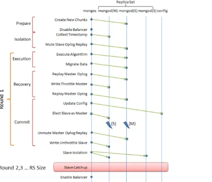
Figure 2.1: Morphus Phases. Arrows represent RPCs. M stands for Master, S for Slave.
2.2.1 MongoDB System Model
We have chosen to incorporate Morphus into a popular sharded key-value store, Mon-goDB [11] v2.4. Beside its popularity, our choice of MonMon-goDB is also driven by its clean documentation, strong user base, and significant development and discussion around it.
A MongoDB deployment consists of three types of servers. The mongod servers store the data chunks themselves – typically, they are grouped into disjoint replica sets. Each replica set contains the same number of (typically 3) servers which are exact replicas of each other, with one of the servers marked as a primary (master), and others acting as secondaries (slaves). The configuration parameters of the database are stored at the config servers. Clients send CRUD (Create, Read, Update, Delete) queries to a front-end server, called mongos. The mongos servers also cache some of the configuration information from the config servers, e.g., in order to route queries they cache mappings from each chunk range to a replica set.
A single database table in MongoDB is called a collection. Thus, a single MongoDB deployment consists of several collections.
2.2.2 Reconfiguration Phases in Morphus
Section 2.3 will describe how new chunks can be allocated to servers in an optimal way. Given such an allocation, we now describe how to i) migrate data, while ii) concurrently supporting operations on this data.
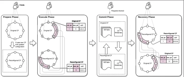
Overview: Morphus allows a reconfiguration operation to be initiated by a system admin-istrator on any collection. Morphus executes the reconfiguration via five sequential phases, as shown in Figure 3.1.
First Morphus prepares for the reconfiguration by creating partitions (with empty new chunks) using the new shard key (Prepare phase). Second, Morphus isolates one secondary server from each replica set (Isolation phase). In the third Execution phase, these secon-daries exchange data based on the placement plan decided by mongos. In the meantime, further operations may have arrived at the primary servers – these are now replayed at the secondaries in the fourth Recovery phase. When the reconfigured secondaries are caught up, they swap places with their primaries (Commit phase).
At this point, the database has been reconfigured and can start serving queries with the new configuration. However, other secondaries in all replica sets need to reconfigure as well – this slave catchup is done in multiple rounds, with the number of rounds equal to the size of the replica set.
Next we discuss the individual phases in detail.
Prepare: The first phase is the Prepare phase, which runs at the mongos front-end. Reads and writes are not affected in this phase, and can continue normally. Concretely, for the shard key change reconfiguration, there are two important steps in this phase:
• Create New Chunks: Morphus queries one of the mongod servers and sets split points for new chunks by using MongoDB’s internal splitting algorithm (for modularity). • Disable Background Processes: We disable background processes of the NoSQL
system which may interfere with the reconfiguration transfer. This includes the MongoDB Balancer, a background thread that periodically checks and balances the number of chunks across replica sets.
Isolation: In order to continue serving operations while the data is being reconfigured, Morphus first performs reconfiguration transfers only among secondary servers, one from each replica set. It prepares by performing two steps:
• Mute Slave Oplog Replay: Normally, the primary server forwards the operation log (called oplog) of all the write operations it receives to the secondary, which then replays it. In the Isolation phase, this oplog replay is disabled at the selected secondaries, but only for the collection being reconfigured – other collections still perform oplog replay.
We chose to keep the secondaries isolated, rather than removed, because the latter would make Recovery more challenging by involving collections not being resharded.
• Collect Timestamp: In order to know where to restart replaying the oplog in the future, the latest timestamp from the oplog is stored in memory by mongos.
Execution: This phase is responsible for making placement decisions (which we will describe in Section 2.3) and executing the resultant data transfer among the secondaries. In the meantime, the primary servers concurrently continue to serve client CRUD operations. Since the selected secondaries are isolated, a consistent snapshot of the collection can be used to run the placement algorithms (Section 2.3) at a mongos server.
Assigning a new chunk to a mongod server implies migrating data in that chunk range from several other mongod servers to the assigned server. For each new chunk, the assigned server creates a separate TCP connection to each source server, “pulls” data from the appropriate old chunks, and commits it locally. All these migrations occur in parallel. We call this scheme of assigning a single socket to each migration as “chunk-based”. The chunk-based strategy can create stragglers, and Section 2.4.1 addresses this problem.
Recovery: At the end of the Execution phase, the secondary servers have data stored according to the new configuration. However, any write (create, update or delete) operations that had been received by a primary server, since the time its secondary was isolated, now need to be communicated to the secondary.
Each primary forwards each item in the oplog to its appropriate new secondary, based on the new chunk ranges. This secondary can be located from our placement plan in the Execution phase, if the operation involved the new shard key. If the operation does not involve the new shard key, it is multicast to all secondaries, and each in turn checks whether it needs to apply it. This mirrors the way MongoDB typically routes queries among replica sets.
However, oplog replay is an iterative process – during the above oplog replay, further write operations may arrive at the primary oplogs. Thus, in the next iteration this delta oplog will need to be replayed. If the collection is hot, then these iterations may take very long to converge. To ensure convergence, we adopt two techniques: i) cap the replay at 2 iterations, and ii) enforce a write throttle before the last iteration. The write throttle is required because of the atomic commit phase that follows right afterwards. The write throttle rejects any writes received during the final iteration of oplog replay. An alternative was to buffer these writes temporarily at the primary and apply them later – however, this would have created another oplog and reinstated the original problem. In any case, the next phase (Commit) requires a write throttle anyway, and thus our approach dovetails with the Commit phase. Read operations remain unaffected and continue normally.
Commit: Finally, we bring the new configuration to the forefront and install it as the default configuration for the collection. This is done in one atomic step by continuing the write throttle from the Recovery phase.
This atomic step consists of two substeps:
• Update Config: The mongos server updates the config database with the new shard key and chunk ranges. Subsequent CRUD operations use the new configuration.
• Elect Slave As Master: Now the reconfigured secondary servers become the new primaries. The old primary steps down and Morphus ensures the secondary wins the subsequent leader election inside each replica set.
To end this phase, the new primaries (old secondaries, now reconfigured) unmute their oplog and the new secondaries (old primaries for each replica set, not yet reconfigured) unthrottle their writes.
Read-Write Behavior: The end of the Commit phase marks the switch to the new shard key. Until this point, all queries with old shard key were routed to the mapped server and all queries with new shard key were multicast to all the servers (normal MongoDB behavior). After the Commit phase, a query with the new shard key is routed to the appropriate server (new primary). Queries which do not use the new shard key are handled with a multicast, which is again normal MongoDB behavior.
Reads in MongoDB offer per-key sequential consistency. Morphus is designed so that it continues to offer the same consistency model for data under migration.
Slave Isolation & Catchup: After the Commit phase, the secondaries have data in the old configuration, while the primaries receive writes in the new configuration. As a result, normal oplog replay cannot be done from a primary to its secondaries. Thus, Morphus isolates all the remaining secondaries simultaneously.
The isolated secondaries catch up to the new configuration via (replica set size - 1) se-quential rounds. Each round consists of the Execution, Recovery and Commit phases shown in Figure 3.1. However, some steps in these phases are skipped – these include the leader election protocol and config database update. Each replica set numbers its secondaries and in the ith round (2≤i≤ replica set size), its ith secondary participates in the reconfigura-tion. The group of ith secondaries reuses the old placement decisions from the first round’s Execution phase – we do so because secondaries need to mirror primaries.
After the last round, all background processes (such as the Balancer) that had been previously disabled are now re-enabled. The reconfiguration is now complete.
Fault-Tolerance: When there is no reconfiguration, Morphus is as fault-tolerant as Mon-goDB. Under ongoing reconfiguration, when there is one failure, Morphus provides similar fault-tolerance as MongoDB – in a nutshell, Morphus does not lose data, but in some cases
the reconfiguration may need to be restarted partially or completely.
Consider the single failure case in detail. Consider a replica set size ofrs≥3. Right after isolating the first secondary in the first round, the old data configuration is still present at (rs−1) servers: current primary and identical (rs−2) idle secondaries. If the primary or an idle secondary fails, reconfiguration remains unaffected. If the currently-reconfiguring sec-ondary fails, then the reconfiguration can be continued using one of the idle secondaries (from that replica set) instead; when the failed secondary recovers it participates in a subsequent reconfiguration round.
In a subsequent round (≥2), if one of the non-reconfigured replicas fails, it recovers and catches up directly with the reconfigured primary. Only in the second round, if the already-reconfigured primary fails, does the entire reconfiguration need to be restarted as this server was not replicated yet. Writes between the new primary election (Round 1 Commit phase) up to its failure, before the second round completes, may be lost. This is similar to the loss of a normal MongoDB write which happens when a primary fails before replicating the data to the secondary. The vulnerability window is longer in Morphus, although this can be reduced by using a backup Morphus server.
With multiple failures, Morphus is fault-tolerant under some combinations. For instance, if all replica sets have at least one new-configuration replica left, or if all replica sets have at least one old-configuration replica left. In the former case, failed replicas can catch up. In the latter case, reconfiguration can be restarted using the surviving replicas.
2.3 ALGORITHMS FOR EFFICIENT SHARD KEY RECONFIGURATIONS
A reconfiguration operation entails the data present in shards across multiple servers to be resharded. The new shards need to be placed at the servers in such a way as to: 1) reduce the total network transfer volume during reconfiguration, and 2) achieve load balance. This section presents optimal algorithms for this planning problem.
We present two algorithms for placement of the new chunks in the cluster. Our first algorithm is greedy and is optimal in the total network transfer volume. However, it may create bottlenecks by clustering many new chunks at a few servers. Our second algorithm, based on bipartite matching, is optimal in network transfer volume among all those strategies that ensure load balance.
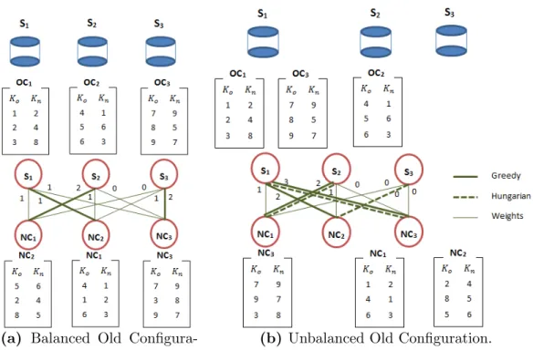
(a) Balanced Old Configura-tion.
(b) Unbalanced Old Configuration.
Figure 2.2: Greedy and Hungarian strategy for shard key change using: (a) Balanced, (b) Unbalanced old chunk configuration. S1 - S3 represent servers. OC1 - OC3 andN C1 - N C3 are old and new chunks respectively. Ko and Kn are old and new shard keys
respectively. Edges are annotated with WN Ci,Sj weights.
2.3.1 Greedy Assignment
The greedy approach considers each new chunk independently. For each new chunk N Ci,
the approach evaluates all the N servers. For each server Sj, it calculates the number of
data items WN Ci,Sj of chunk N Ci that are already present in old chunks at server Sj. The
approach then allocates each new chunkN Ci to that serverSj which has the maximum value
of WN Ci,Sj, i.e.,argmaxS∗(WN Ci,Sj). As chunks are considered independently, the algorithm
produces the same output irrespective of the order in which chunks are considered by it. The calculation of WN Ci,Sj values can be performed in parallel at each server Sj, after
servers are made aware of the new chunk ranges. A centralized server collects all theWN Ci,Sj
values, runs the greedy algorithm, and informs the servers of the allocation decisions. Lemma 2.1 The greedy algorithm is optimal in total network transfer volume.
Proof: The proof is by contradiction. Consider an alternative optimal strategy A that assigns at least one new chunk N Ci to a server Sk different from S0 = argmaxS∗(WN Ci,Sj),
such that WN Ci,S0 > WN Ci,Sk – if there is no such N Ci, then A produces the same total
re-assigned toS0, one can achieve a reconfiguration that has a lower network transfer volume than A, a contradiction.
For each of them new chunks, this algorithm iterates through all theN servers. Thus its complexity is O(m.N), linear in the number of new chunks and cluster size.
To illustrate the greedy scheme in action, Fig. 2.2 provides two examples for the shard key change operation. In each example, the database has 3 old chunks OC1 −OC3 each containing 3 data items. For each data item, we show the old shard key Ko and the new
shard key Kn (both in the ranges 1-9). The new configuration splits the new key range
evenly across 3 chunks shown as N C1−N C3.
In Fig. 2.2a, the old chunks are spread evenly across servers S1−S3. The edge weights in the bipartite graph show the number of data items of N Ci that are local at Sj, i.e.,WN Ci,Sj
values. Thick lines show the greedy assignment.
However, the greedy approach may produce an unbalanced chunk assignment for skewed bipartite graphs, as in Fig. 2.2b. While the greedy approach minimizes network transfer volume, it assigns new chunks N C2 and N C3 to server S1, while leaving server S3 empty.
2.3.2 Load Balance via Bipartite Matching
Load balancing chunks across servers is important for several reasons: i) it improves read/write latencies for clients by spreading data and queries across more servers; ii) it re-duces read/write bottlenecks; iii) it rere-duces the tail of the reconfiguration time, by preventing allocation of too many chunks to any one server.
Our second strategy achieves load balance by capping the number of new chunks allocated to each server. With m new chunks, this per-server cap is dm/Ne chunks. We then create a bipartite graph with two sets of vertices – top and bottom. The top set consists of dm/Ne vertices for each of the N servers in the system; denote the vertices for server Sj as
S1
j −S
dm/Ne
j . The bottom set of vertices consist of the new chunks. All edges between a top
vertex Sk
j and a bottom vertex N Ci have an edge cost equal to |N Ci| −WN Ci,Sj i.e., the
number of data items that will move to server Sj if new chunkN Ci were allocated to it.
Assigning new chunks to servers in order to minimize data transfer volume now becomes a bipartite matching problem. Thus, we find the minimum weight matching by using the classical Hungarian algorithm [53]. The complexity of this algorithm isO((N.V+m).N.V.m) where V = dm/Ne chunks. This reduces to O(m3). The greedy strategy of Section 2.3.1 becomes a special case of this algorithm with V =m.
Lemma 2.2 Among all load-balanced strategies that assign at most V =dm/Ne new chunks to any server, the Hungarian algorithm is optimal in total network transfer volume.
Proof: The proof follows from the optimality of the Hungarian algorithm [53].
Fig. 2.2b shows the outcome of the bipartite matching algorithm using dotted lines in the graph. While it incurs the same overall cost as the greedy approach, it additionally provides the benefit of a load-balanced new configuration, where each server is allocated exactly one new chunk.
While we focus on the shard key change, this technique can also be used for other recon-figurations like changing shard size, or cluster scale out and scale in. The bipartite graph would be drawn appropriately (depending on the reconfiguration operation), and the same matching algorithm used. For purpose of concreteness, the rest of the chapter focuses on shard key change.
Finally, although we have used datasize (number of key-value pairs) as the main cost metric. Instead we could use traffic to key-value pairs as the cost metric, and derive edge weights in the bipartite graph (Fig. 2.2) from these traffic estimates. Hungarian approach on this new graph would balance out traffic load, while trading off optimality – further exploration of this variant is beyond our scope in this chapter.
2.4 NETWORK-AWARENESS
In this section, we describe how we augment the design of Section 2.2 in order to handle two important concerns: awareness to the topology of a datacenter, and geo-distributed settings.
Figure 2.3: Execution phase CDF for chunk-based strategy on Amazon 500 MB database in tree network topology with 9 mongod servers spread evenly across 3 racks.
2.4.1 Awareness to Datacenter Topology
Datacenters use a wide variety of topologies, the most popular being hierarchical, e.g., a typical two-level topology consists of a core switch and multiple rack switches. Others that
are commonly used in practice include fat-trees [54], CLOS [55], and butterfly [56].
Our first-cut data migration strategy discussed in Section 2.2 waschunk-based: it assigned as many sockets (TCP streams) to a new chunk C at its destination server as there are source servers for C i.e., it assign one TCP stream per server pair. Using multiple TCP streams per server pair has been shown to better utilize the available network bandwidth [57]. Further, the chunk-based approach also results instragglersin the execution phase as shown in Figure 2.3. Particularly, we observe that 60% of the chunks finish quickly, followed by a 40% cluster of chunks that finish late.
To address these two issues, we propose a weighted fair sharing (WFS) scheme that takes both data transfer size and network latency into account. Consider a pair of servers i and j, where i is sending some data to j during the reconfiguration. Let Di,j denote the total
amount of data that i needs to transfer to j, and Li,j denote the latency in the shortest
network path from i to j. Then, we set Xi,j, the weight for the flow from server i to j, as
follows:
Xi,j ∝Di,j ×Li,j (2.1)
In our implementation, the weights determine the number of sockets that we assign to each flow. We assign each destination serverj a total number of sockets Xj =K×
P iDi,j P
i,jDi,j,
where K is the total number of sockets throughout the system. Thereafter each destination server j assigns each source server i a number of sockets, Xi,j =Xj ×PCi,j
iCi,j.
However,Xi,j may be different from the number of new chunks that j needs to fetch from
i. If Xi,j is larger, we treat each new chunk as a data slice, and iteratively split the largest
slice into smaller slices untilXi,j equals the total number of slices. Similarly, ifXi,j is smaller,
we use iterative merging of the smallest slices. Finally, each slice is assigned a socket for data transfer. Splitting or merging slices is only for the purpose of socket assignment and to speed up data transfer; it does not affect the final chunk configuration which was computed in the Prepare phase.
Our approach above could have used estimates of available bandwidth instead of latency estimates. We chose the latter because: i) they can be measured with a lower overhead, ii) they are more predictable over time, and iii) they are correlated to the effective bandwidth.
2.4.2 Geo-Distributed Settings
So far, Morphus has assumed that all its servers reside in one datacenter. However, typical NoSQL configurations split servers across geo-distributed datacenters for fault-tolerance. Naively using the Morphus system would result in bulk transfers across the wide-area network and prolong reconfiguration time.
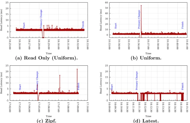
(a) Read Only (Uniform). (b) Uniform.
(c) Zipf. (d) Latest.
Figure 2.4: Read Latency for: (a) Read only operations (no writes), and three read-write workloads modeled after YCSB: (b) Uniform, (c) Zipf, and (d) Latest. Times shown are hh:mm:ss. Failed reads are shown as negative latencies. Annotated “Pri-mary Change” point marks the start of the leader election protocol in the first round.
To address this, we localize each stage of the data transfer to occur within a datacenter. We leverage MongoDB’s server tags [58] to tag each replica set member with its datacenter identifier. Morphus then uses this information to select replicas, which are to be reconfigured together in each given round, in such a way that they reside within the same datacenter. If wide-area transfers cannot be eliminated at all, Morphus warns the database admin.
One of MongoDB’s invariants for partition-tolerance requires each replica set to have a voting majority at some datacenter [58]. In a three-member replica set, two members (primary and secondary-1) must be at one site while the third member (secondary-2) could be at a different site. Morphus obeys this requirement by selecting that secondary for the first round which is co-located with the current primary. In the above example, Morphus would select the secondary-1 replicas for the first round of reconfiguration. In this way, the invariant stays true even after the leader election in the Commit phase.
2.5 EVALUATION
• How much does Morphus affect read and write operations during reconfiguration? • For shard key change, how do the Greedy and Hungarian algorithms of Section 2.3
compare?
• How does Morphus scale with data size, operation injection rate, and cluster size? • How much benefit can we expect to get from the network-aware (datacenter topology
and geo-distributed) strategies?
2.5.1 Setup
Data Set: We use the dataset of Amazon reviews as our default collection [59]. Each data item has 10 fields. We chooseproductID as the old shard key,userIDas the new shard key, while update operations use these two fields and a price field. Our default database size is 1 GB (we later show scalability with data size).
Cluster: The default Morphus cluster uses 10 machines. These consist of one mongos (front-end), and 3 replica sets, each containing a primary and two secondaries. There are 3 config servers, each co-located on a physical machine with a replica set primary – this is an allowed MongoDB installation. All physical machines are d710 Emulab nodes [60] with a 2.4 GHz processor, 4 cores, 12 GB RAM, 2 hard disks of 250 GB and 500 GB, 64 bit CentOS 5.5, and connected to a 100 Mbps LAN switch.
Workload Generator: We implemented a custom workload generator that injects YCSB-like workloads via MongoDB’s pymongo interface. Our default injection rate is 100 ops/s with 40% reads, 40% updates, and 20% inserts. To model realistic key access patterns, we select keys for each operation via one of three YCSB-like [61] distributions: 1) Uniform (de-fault), 2) Zipf, and 3) Latest. For Zipf and Latest distributions we employ a shape parameter α = 1.5. The workload generator runs on a dedicated pc3000 node in Emulab running a 3GHz processor, 2GB RAM, two 146 GB SCSI disks, 64 bit Ubuntu 12.04 LTS.
Morphus default settings: Morphus was implemented in about 4000 lines of C++ code. The code is publicly available at http://dprg.cs.uiuc.edu/downloads. A demo of Mor-phus can be found at https://youtu.be/0rO2oQyyg0o. For the evaluation, each plotted datapoint is an average of at least 3 experimental trials, shown along with standard deviation bars.
2.5.2 Read Latency
Fig. 2.4 shows the timelines for four different workloads during the reconfiguration, lasting between 6.5 minutes to 8 minutes. The figure depicts the read latencies for the reconfigured
database table (collection), with failed reads shown as negative latencies. We found that read latencies for collections not being reconfigured were not affected and we do not plot these.
Fig. 2.4a shows the read latencies when there are no writes (Uniform read workload). We observe unavailability for a few seconds (from time t =18:28:21 to t =18:28:29) during the Commit phase when the primaries are being changed. This unavailability lasts only about 2% of the total reconfiguration time. After the change, read latencies spike slightly for a few reads but then settle down. Figs. 2.4b to 2.4d plot the YCSB-like read-write workloads. We observe similar behavior as Fig. 2.4a.
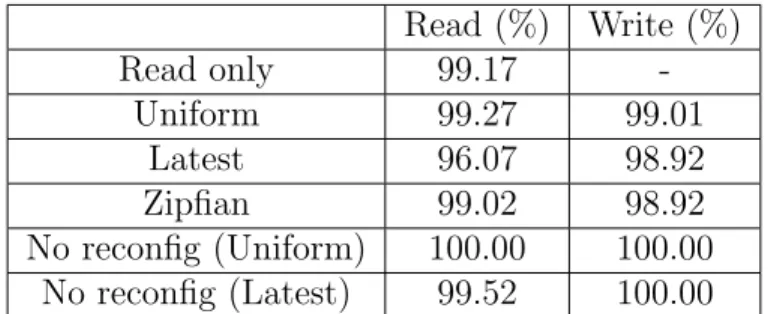
Read Write Read Only 99.9
-Uniform 99.9 98.5 Latest 97.2 96.8 Zipf 99.9 98.3
Table 2.1: Percentage of Reads and Writes that Succeed under Reconfiguration. (Figs. 2.4 and 2.6)
Fig. 2.4d indicates that the Latest workload incurs a lot more failed reads. This is because the keys that are being inserted and updated are the ones more likely to be read. However, since some of the insertions fail due to the write throttles at various points during the reconfiguration process (t=14:11:20 to t=14:11:30, t=14:13:15 tot =14:13:20, t=14:15:00 to t =14:15:05 from Fig. 2.6c), this causes subsequent reads to also fail. However, these lost reads only account for 2.8% of the total reads during the reconfiguration time – in particular, Table 2.1 (middle column) shows that 97.2% of the reads succeed under the Latest workload. The availability numbers are higher at three-9’s for Uniform and Zipf workload, and these are comparable to the case when there are no insertions. We conclude that unless there is temporal and spatial (key-wise) correlation between writes and reads (i.e., Latest workloads), the read latency is not affected much by concurrent writes. When there is correlation, Morphus mildly reduces the offered availability.
To flesh this out further, we plot in Fig. 2.5 the CDF of read latencies for these four settings, and when there is no reconfiguration (Uniform workload). Notice that the horizontal axis is logarithmic scale. We only consider latencies for successful reads. We observe that the 96th percentile latencies for all workloads are within a range of 2 ms. The median (50th percentile) latency for No Reconfiguration is 1.4 ms, and this median holds for both the Read only (No Write) and Uniform workloads. The medians for Zipf and Latest workloads are lower at 0.95 ms. This lowered latency is due to two reasons: caching at the mongod servers for the frequently-accessed keys, and in the case of Latest the lower percentage of
Figure 2.5: CDF of Read Latency. Read latencies under no reconfiguration (No Reconf ), and four under-reconfiguration workloads.
successful reads.
We conclude that under reconfiguration, the read availability provided by Morphus is high (two to three 9’s of availability), while the latencies of successful read operations do not degrade compared to the scenario when there is no reconfiguration in progress.
2.5.3 Write Latency
We next plot the data for write operations, i.e., inserts, updates and deletes.
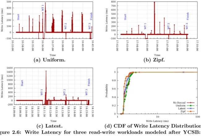
Figs. 2.6a to 2.6c show writes in the same timelines as Figs. 2.4b to 2.4d. We observe that many of the failed writes occur during one of the write throttling periods (annotated as “WT”). Recall from Section 2.2.2 that there are as many write throttling periods as the replica set size, with one throttle period at the end of each reconfiguration round.
Yet, the number of writes that fail is low: Table 2.1 (last column) shows that for the Uniform and Zipf workloads, fewer than 2% writes fail. The Latest workload again has a slightly higher failure rate since a key that was attempted to be written (unsuccessfully) is more likely to be attempted to be written again in the near future. Yet, the write failure rate of 3.2% is reasonably low.
To flesh this out further, the CDF of the write latencies (ignoring failed writes) is shown in Fig. 2.6d. The median for writes when there is no reconfiguration (Uniform workload) in progress is 1.45 ms. The Zipf and Latest workloads have a similar median latency. Uni-form has a slightly higher median latency at 1.6 ms – this is because 18% of the updates experience high latencies. This is due to Greedy’s skewed chunk assignment plan (discussed and improved in Section 2.5.4). Greedy assigns a large percentage of new chunks to a single replica set, which thus receives most of the new write traffic. This causes MongoDB’s peri-odic write journal flushes4 to take longer. This in turn delays the new writes arriving around
(a) Uniform. (b) Zipf.
(c) Latest. (d) CDF of Write Latency Distribution. Figure 2.6: Write Latency for three read-write workloads modeled after YCSB: (a) Uniform, (b) Zipf, and (c) Latest. Times shown are hh:mm:ss. Failed writes are shown as negative latencies. Annotations marked “WT” indicate the start of each write throttle phase. (d) CDF of Write Latency Distribution for no reconfiguration (No Reconf ) and three under-reconfiguration workloads.
the journal flush timepoints. Many of the latency spikes observed in Figs. 2.6a to 2.6c arise from this journaling behavior.
We conclude that under reconfiguration, the write availability provided by Morphus is high (close to two 9’s), while latencies of successful writes degrade only mildly compared to when there is no reconfiguration in progress.
2.5.4 Hungarian vs. Greedy Reconfiguration
Section 2.3 outlined two algorithms for the shard key change reconfiguration – Hungarian and Greedy. We implemented both these techniques into Morphus – we call these variants as Morphus-H and Morphus-G respectively. For comparison, we also implemented a random chunk assignment scheme called Morphus-R.
Fig. 2.7 compares these three variants under two scenarios. The uncorrelated scenario (left pair of bars) uses a synthetic 1 GB dataset where for each data item, the value for its new shard key is selected at random and uncorrelated to its old shard key’s value. The plot shows
Figure 2.7: Greedy (Morphus-G) vs. Hungarian (Morphus-H) Strategies for shard key change. Uncorrelated: random old and new shard key. Correlated: new shard key is reverse of old shard key.
the total reconfiguration time including all the Morphus phases. Morphus-G is 15% worse than Morphus-H and Morphus-R. This is because Morphus-G ends up assigning 90% new chunks to a single replica set which results in stragglers during the Execution and Recovery phases. The underlying reason for the skewed assignment can be attributed to MongoDBs split algorithm which we use modularly. The algorithm partitions the total data size instead of total record count. When partitioning the data using the old shard key, this results in some replica sets getting a larger number of records than others. Morphus-R performs as well as Morphus-H because by randomly assigning chunks to servers, it also achieves load balance
The correlated scenario in Fig. 2.7 (right pair of bars) shows the case where new shard keys have a reversed order compared to old shard keys. That is, with M data items, old shard keys are integers in the range [1, M], and the new shard key for each data item is set as =M−old shard key. This results in data items that appeared together in chunks continuing to do so (because chunks are sorted by key). Morphus-R is 5x slower than both Morphus-G and Morphus-H. Randomly assigning chunks can lead to unnecessary data movement. In the correlated case, this effect is accentuated. Morphus-G is 31% faster than Morphus-H. This is because the total transfer volume is low anyway in Morphus-G due to the correlation, while Morphus-H additionally attempts to load-balance.
We conclude that i) the algorithms of Section 3 give an advantage over random assignment, especially when old and new keys are correlated, and ii) Morphus-H performs reasonably well in both the correlated and uncorrelated scenario and should be preferred over Morphus-G and Morphus-R.
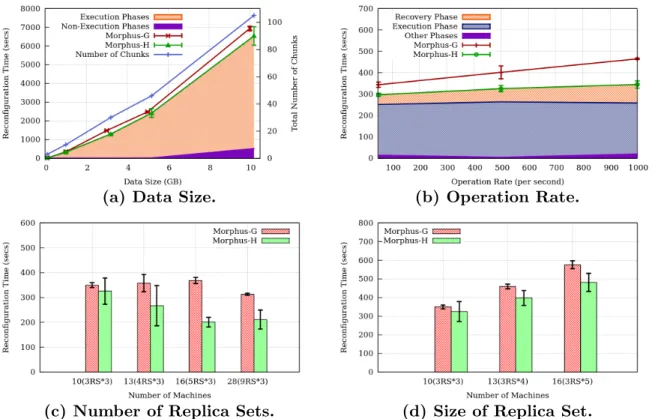
(a) Data Size. (b) Operation Rate.
(c) Number of Replica Sets. (d) Size of Replica Set.
Figure 2.8: Morphus Scalability with: (a) Data Size, also showing Morphus-H phases, (b) Operation injection rate, also showing Morphus-H phases, (c) Number of replica sets, and (d) Replica set size.
2.5.5 Scalability
We explore scalability of Morphus along three axes – database size, operation injection rate, and size of cluster. These experiments use the Amazon dataset.
Database Size: Fig. 2.8a shows the reconfiguration time at various data sizes from 1 GB to 10 GB. There were no reads or writes injected. For clarity, the plotted data points are perturbed slightly horizontally.
Firstly, Fig. 2.8a shows that Morphus-H performs slightly better than Morphus-G for the real-life Amazon dataset. This is consistent with our observations in Section 2.5.4 since the Amazon workload is closer to the uncorrelated end of the spectrum.
Secondly, the total reconfiguration time appears to increase superlinearly beyond 5 GB. This can be attributed to two factors. First, reconfiguration time grows with the number of chunks – this number is also plotted, and we observe that it grows superlinearly with datasize. This is again caused by MongoDB’s splitting code 5. Second, we have reused MongoDB’s data transfer code, which relies on cursors (i.e., iterators), which are not the best approach for bulk transfers. We believe this can be optimized further by writing a
module for bulk data transfer – yet, we reiterate that this is orthogonal to our contributions: even during the (long) data transfer time, reads and writes are still supported with several 9s of availability (Table 1). Today’s existing approach of exporting/reimporting data with the database shut down, leads to long unavailability periods – at least 30 minutes for 10 GB of data (assuming 100% bandwidth utilization). In comparison, Morphus is unavailable in the worst-case (from Table 1) for 3.2% ×2 hours = 3.84 minutes, which is an improvement of about 10x.
Fig. 2.8a also illustrates that a significant fraction of the reconfiguration time is spent migrating data, and this fraction grows with increasing data size – at 10 GB, the data transfer occupies 90% of the total reconfiguration time. This indicates that Morphus’ overheads fall and will become relatively small at large data sizes.
We conclude that the reconfiguration time incurred by Morphus scales linearly with the number of chunks in the system and that the overhead of Morphus falls with increasing data size.
Operation Injection Rate: An important concern with Morphus is how fast it plays “catch up” when there are concurrent writes during the reconfiguration. Fig. 2.8b plots the reconfiguration time against the write rate on 1 GB of Amazon data. In both Morphus-G and Morphus-H, we observe a linear increase. More concurrent reads and writes slow down the overall reconfiguration process because of two reasons: limited bandwidth available for the reconfiguration data transfers, and a longer oplog that needs to be replayed during the Recovery Phase. However, this increase is slow and small. A 20-fold increase in operation rate from 50 ops/s to 1000 ops/s results in only a 35% increase in reconfiguration time for Morphus-G and a 16% increase for Morphus-H.
To illustrate this further, the plot shows the phase breakdown for Morphus-H. The Recov-ery phase grows as more operations need to be replayed. Morphus-H has only a sublinear growth in reconfiguration time. This is because of two factors. First Morphus-H balances the chunks out more than Morphus-G, and as a result the oplog replay has a shorter tail. Second, there is an overhead in Morphus-H associated with fetching the oplog via the Mon-goDB cursors (iterators) – at small write rates, this overhead dominates but as the write rate increases, the contribution of this overhead drops off. This second factor is present in Morphus-G as well, however it is offset by the unbalanced distribution of new chunks.
We conclude that Morphus catches up quickly when there are concurrent writes, and that its reconfiguration time scales linearly with write operation injection rate.
Cluster Size: We investigate cluster size scalability along two angles: number of replica sets, and replica set size. Fig. 2.8c shows that as the number of replica sets increases from 3 to 9 (10 to 28 servers), both Morphus-G and Morphus-H eventually become faster with
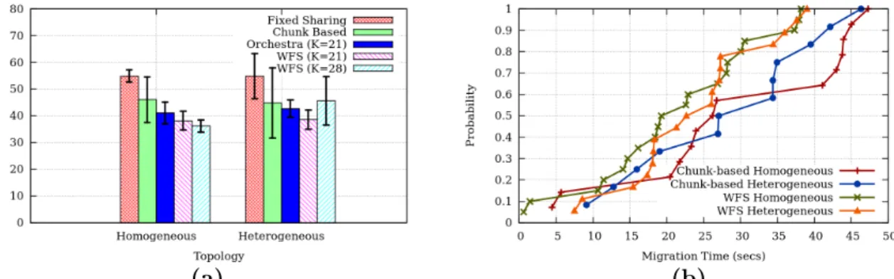
(a) (b)
Figure 2.9: (a) Execution Phase Migration time for five strategies: (i) Fixed Sharing (FS), (ii) Chunk-based strategy, (iii) Orchestra with K = 21, (iv) WFS with K = 21, and (v) WFS with K = 28. (b) CDF of total reconfiguration time in chunk-based strategy vs. WFS with K = 28.
scale. This is primarily because of increasing parallelism in the data transfer, while the amount of data migrating over the network grows much slower – with N replica sets, this latter quantity is approximately a fraction N−1
N of data. While Morphus-G’s completion time
is high at a medium cluster size (16 servers) due to its unbalanced assignment, Morphus-H shows a steady improvement with scale and eventually starts to plateau as expected.
Next, Fig. 2.8d shows the effect of increasing replica set size. We observe a linear increase for both Morphus-G and Morphus-H. This is primarily because there are as many rounds inside a reconfiguration run as there are machines in a replica set.
We conclude that Morphus scales reasonably with cluster size – in particular, an increase in number of replica sets improves its performance.
2.5.6 Effect of Network Awareness
Datacenter Topology-Awareness: First, Fig. 2.9a shows the length of the Execution phase (using a 500 MB Amazon collection) for two hierarchical topologies, and five migration strategies. The topologies are: i) homogeneous: 9 servers distributed evenly across 3 racks, and ii) heterogeneous: 3 racks contain 6, 2, and 1 servers respectively. The switches are Emulab pc3000 nodes and all links are 100 Mbps. The inter-rack and intra-rack latencies are 2 ms and 1 ms respectively. The five strategies are: a) Fixed sharing, with one socket assigned to each destination node, b) chunk-based approach (Section 2.4.1), c) Orchestra [57] with K = 21, d) WFS with K = 21 (Section 2.4.1), and e) WFS with K = 28.
We observe that in the homogeneous clusters, WFS strategy with K = 28 is 30% faster than fixed sharing, and 20% faster than the chunk-based strategy. Compared to Orchestra which only weights flows by their data size, taking the network into account results in a 9%
improvement in WFS with K = 21. IncreasingK from 21 to 28 improves completion time in the homogeneous cluster, but causes degradation in the heterogeneous cluster. This is because a higher K results in more TCP connections, and at K = 28 this begins to cause congestion at the rack switch of 6 servers. Second, Fig. 2.9b shows that compared to Fig. 2.3 (from Section 2.4), Morphus’ network-aware WFS strategy has a shorter tail and finishes earlier. Network-awareness lowers the median chunk finish time by around 20% in both the homogeneous and heterogeneous networks.
We conclude that WFS strategy improves performance compared to existing approaches, and K should be chosen high enough but without causing congestion.
Geo-Distributed Setting: Table 2.2 shows the benefit of the tag-aware approach of Mor-phus (Section 2.4.2). The setup has two datacenters with 6 and 3 servers, with intra- and inter-datacenter latencies of 0.07 ms and 2.5 ms respectively (based on [62]) and links with 100 Mbps bandwidth. For 100 ops/s workload on 100 MB of reconfigured data, tag-aware Morphus improves performance by over 2x when there are no operations and almost 3x when there are reads and writes concurrent with the reconfiguration.
Without With
Read/Write Read/Write Tag-Unaware 49.074s 64.789s
Tag-Aware 21.772s 23.923s
Table 2.2: Reconfiguration Time in the Geo-distributed setting.
2.5.7 Large Scale Experiment
In this experiment, we increase data and cluster size simultaneously such that the amount of data per replica set is constant. We ran this experiment on Google Cloud [63]. We used n1-standard-4 VMs each with 4 virtual CPUs and 15 GB of memory. The disk capacity was 1 GB and the VMs were running Debian 7. We generated a synthetic dataset similar to the one used in Section 2.5.4. Morphus-H was used for reconfiguration with WFS migration scheme and K = number of old chunks.
Fig. 2.10 shows a sublinear increase in reconfiguration time as data and cluster size in-creases. Note that x-axis uses log scale. In the Execution phase, all replica sets communicate among each other for migrating data. As the number of replica sets increases with cluster size, the total number of connections increases leading to network congestion. Thus, the Execution phase takes longer.
The amount of data per replica set affects reconfiguration time super-linearly. On the contrary, cluster size has a sublinear impact. In this experiment, the latter dominates as the