Dictionary Compression in Point Cloud Data Management

(1)

Anastasia Ailamaki

EPFL & RAW Labs SA [email protected]

ABSTRACT

Nowadays, massive amounts of point cloud data can be collected thanks to advances in data acquisition and processing technologies like dense image matching and airborne LiDAR (Light Detection and Ranging) scanning. With the increase in volume and preci-sion, point cloud data offers a useful source of information for natural resource management, urban planning, self-driving cars and more. At the same time, the scale at which point cloud data is produced, introduces management challenges: it is important to achieve efficiency both in terms of querying performance and space requirements. Traditional file-based solutions to point cloud management offer space efficiency, however, cannot scale to such massive data and provide the same declarative power as a database management system (DBMS).

In this paper, we propose a time- and space-efficient solution to storing and managing point cloud data in main memory column-store DBMS. Our solution, Space-Filling Curve Dictionary-Based Compression (SFC-DBC), employs dictionary-based compression in the spatial data management domain and enhances it with indexing capabilities by using space-filling curves. It does so by constructing the space-filling curve over a compressed, artificially introduced 3D dictionary space. Consequently, SFC-DBC significantly optimizes query execution, and yet it does not require additional storage resources, compared to traditional dictionary-based compression. With respect to space-filling curve-based approaches, it minimizes storage footprint and increases resilience to skew. As a proof of concept, we develop and evaluate our approach as a research pro-totype in the context of SAP HANA. SFC-DBC outperforms other dictionary-based compression schemes by up to 61% in terms of space and up to 9.4x in terms of query performance.

CCS CONCEPTS

•Information systems→Data compression;Multidimensional range search;Main memory engines; Data analytics;

Permission to make digital or hard copies of all or part of this work for personal or classroom use is granted without fee provided that copies are not made or distributed for profit or commercial advantage and that copies bear this notice and the full citation on the first page. Copyrights for components of this work owned by others than ACM must be honored. Abstracting with credit is permitted. To copy otherwise, or republish, to post on servers or to redistribute to lists, requires prior specific permission and/or a fee. Request permissions from [email protected].

SIGSPATIAL’17, November 7–10, 2017, Los Angeles Area, CA, USA

KEYWORDS

Point Cloud, Multidimensional Data Access Methods, Data Com-pression, Spatial Data Management

ACM Reference format:

Mirjana Pavlovic, Kai-Niklas Bastian, Hinnerk Gildhoff, and Anastasia Aila-maki. 2017. Dictionary Compression in Point Cloud Data Management. In

Proceedings of SIGSPATIAL’17, Los Angeles Area, CA, USA, November 7–10, 2017,10 pages.

https://doi.org/10.1145/3139958.3139969

1 INTRODUCTION

Recent advances in laser technology [30] and image processing [8] have evolved the importance of point cloud data and challenges considering its management. The ease of gathering 3D point cloud data, together with its public availability, have made it more attrac-tive to users. During recent years, many datasets have been released as open data. These datasets offer a useful source of information for natural resource management, urban planning and more, by modeling point data through up to 26 properties such asx,y, andz coordinates, angle of scan, and color. One such prominent dataset is the second national height map of the Netherlands (AHN2) [18], which was acquired through airborne and terrestrial scanning and contains 640 billion points.

Given the massive amounts of point cloud data, it is important to achieve efficiency in terms of both querying performance and storage footprint. Traditional solutions to point cloud data manage-ment are file-based: points are stored in files in a predefined format and processed by application-specific algorithms. These solutions typically employ efficient compression schemes, but 1) face scala-bility problems with respect to the increasing number and size of files to process and 2) lack the declarative power of a DBMS [1, 29]. Therefore, research in this area has recently shifted towards DBMSs, as many of the data management challenges encountered with the increasing point cloud data size have already been addressed in DBMS solutions [29]. Recent work [1, 6, 12, 29] illustrates the po-tential of column-store DBMSs to meet point cloud management requirements, but focuses mostly on processing performance and ignores storage considerations.

This paper presents a design for storing and managing point cloud data in the context of column-store DBMSs, that is driven both by time and space efficiency requirements. More specifically, we employ dictionary-based compression (DBC) – a compression method frequently used in main-memory column stores [5, 13] – in the spatial domain and enhance it with indexing capabilities, mini-mizing both space and time requirements. The resulting technique,

(2)

Space-Filling Curve Dictionary-Based Compression (SFC-DBC), compresses point cloud data using DBC, leveraging the frequent repetition of the values forx,y, andzcoordinates across point cloud entries; this property is particularly evident for data obtained through image matching processing as it inherits the grid-like struc-ture of images. DBC significantly minimizes space requirements. However, it is agnostic to spatial data properties. To preserve and exploit spatial data properties and thus optimize further for query execution, we combine DBC with Space-Filling Curve (SFC) order to design a new compression scheme.

According to our compression scheme, a point cloud entry is represented through its position in an artificially introduced 3D dictionary space and indexed using a SFC order. As we illustrate in our experimental results, SFC-DBC does not require additional space resources, and yet significantly optimizes query execution, compared to traditional DBC. With respect to the traditional space-filling curve-based approaches, it minimizes storage footprint and increases resilience to skew.

In particular, our contributions are:

•We explore different solutions to store and manage point

cloud data, having dictionary-based compression as a first-class citizen.

•We develop SFC-DBC, a novel encoding scheme that

em-ploys dictionary-based compression in the spatial domain, enhancing it with indexing capabilities to provide time and space efficiency properties.

•We develop and evaluate our approach as a research

proto-type in the context of SAP HANA [5]. SFC-DBC outperforms other dictionary-based compression schemes by up to 61% in terms of space and up to 9.4x in terms of query performance. The remainder of the paper is structured as follows. We provide the background of our work, i.e., discuss DBC and SFC order in the context of point cloud data management in Section 2. We introduce our approach in Section 3 and discuss experimental evaluation in Section 4. Finally, we give an overview of related work in Section 5 and draw conclusions in Section 6.

2 BACKGROUND

Our proposed solution combines dictionary-based compression (DBC) and space-filling curve (SFC) order to efficiently store and manage point cloud data. Therefore, in this section we discuss the choice of DBC and SFC order, describe traditional approaches to these techniques and outline their shortcoming and challenges when it comes to point cloud data management.

2.1 Dictionary-based Compression

Two major technologies that are used for point cloud data acqui-sition are LiDAR [30] and dense image matching [8]. LiDAR is fundamentally a distance technology that uses an emitted laser pulse to determine an object’s distance from a sensor, while image processing technology acquires point cloud data through dense image matching of multiple overlapping aerial images. With recent technological advancements, dense image matching has gained popularity as it offers the same capabilities as LiDAR, at a lower price and finer resolution [8]. Whether the point cloud data is ob-tained through LiDAR or image matching technology, the values

value vid 0.3 0 0.5 1 1.2 2 2.3 3 10.1 4 . . . vid 4 1 7 3 4 2 9 … X IVz binary search scan value vid 0.3 0 0.5 1 0.9 2 2.3 3 2.4 4 . . . vid 5 1 4 3 4 3 1 … Z value vid 0.1 0 1.5 1 1.2 2 3.3 3 20.1 4 . . . vid 9 2 6 2 4 5 0 … Y IVx IVy 7 dictionary index vector

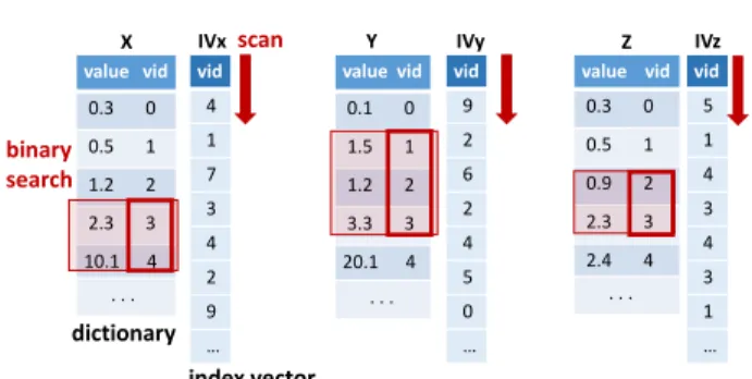
Figure 1: An example of range query execution over a dictionary-based representation of point cloud data.

forx,y, andzcoordinates (not the points themselves) repeat across point cloud entries frequently. The data obtained through image matching processing by default has these properties as it inherits the grid-like structure of images, while LiDAR data obtains these characteristics as the result of typically employed post-processing steps (e.g., thinning-out of data) [25, 30]. We take advantage of these patterns in data distribution by employing DBC, a method frequently used in main-memory column stores [5, 13].

Dictionary-based Compression.DBC compresses a column

by mapping its domain to a list of continuous integer values, i.e., replacing wide values in the attribute domain with smaller codes. Its simplest form consists of a dictionary and an index vector (IV). The dictionary stores the sorted distinct values of the column domain, while theIVmaps each point to its position in the dictionary.

When naively applied in the context of point clouds, DBC rep-resents point cloud data as three independent columns – one for each dimension of the 3D space – composed of a dictionary and an IV. The dictionary stores the sorted distinct values for the corre-sponding dimension and theIVmaps the point to its corresponding position in the dictionary, as illustrated in Figure 1. A 3D range query is executed by performing binary search on the dictionary of each dimension to identify values and their corresponding posi-tions in dictionaries that intersect with the query range. The binary search is followed by a scan of the correspondingIVto identify the records that match the identified dictionary position.

Challenges.Although the baseline DBC solution to store and

query point cloud data is a straightforward one, it wastes com-putational resources as it does not leverage the spatial properties of data. More precisely, it treats and consequently processes the dimensions and points independently, leading to a full scan of the IVsfor each dimension. As we illustrate in our experiments (Section 4), even optimized scans of vector data require considerable time when processing massive point cloud datasets.

Therefore, to optimize this strategy we leverage a correlation within and across point cloud entries. A point cloud entry is rep-resented withx,y, andzcoordinates that are correlated, i.e., they describe a point in 3D space. Moreover, there is a correlation across the points: points close in 3D space will be frequently processed (e.g., queried) together. Therefore, we take advantage of this property and organize data to persevere spatial proximity. Consequently, we can restrict a search range using an index structure (that combines all 3 dimensions) and improve the data access patterns. However, a challenge is to achieve this in both time and space-efficient manner, as an index-like structure normally increases the storage footprint.

(3)

Y 72 70.7 55 37.2 17 1.7 1.5 0.1 0.1 1 1.2 2 26 72 88 99 3 Y dictionary X dictionary P(0.1, 1.5) SFCcodes (0, 0) 0 1 2 3 Y 3 2 1 0 0 1 0 1 0 1 0 1 Y 11 0 1 0 1 0 1 0 + offsets(0, 1) dictionary space SFC_IV

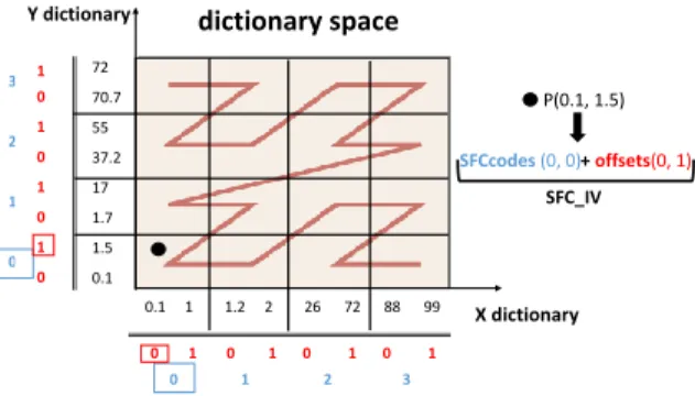
Figure 2: Dictionary space, 2D illustration.

2.2 Space-filling Curves

A common way to preserve and exploit spatial data properties is by using Space-filling Curves (SFC) [14–16, 21, 29]. SFC-based organization transforms data from a multi- to a one-dimensional domain using a SFC to impose a total, 1D order by visiting all the points in ad-dimensional grid exactly once. The Hilbert curve [10], the Gray-code curve [3], and the Z-order [20] are examples of SFC curves that are effective in preserving spatial proximity [4, 10, 17]. We opt to use a SFC-based organization to preserve and exploit spatial data properties due to its suitability for column-store DBMS. By transforming data to a 1D domain, we do not preserve spatial proximity to the same extent as with multi-dimensional data structures, however, we retain the ability to employ efficient scans of vector data. Simplicity and efficiency in the preprocessing step are additional benefits of this approach. In the following we describe the traditional approach to organize and query data using SFC. We focus on range queries as they are broadly used in many applications and are also the fundamental building block for many other spatial queries (e.g.,k-nearest neighbor queries [11]).

SFC Organization.SFC order reorganizes data in three steps:

(1) Partition the dataset’s universe with a uniform grid and assign to each cell a value on the space-filling curve (SFCcode), (2) Assign SFCcodeto every point cloud entry according to the grid cell they belong to, where multiple point cloud entries can map to the same SFCcodevalue, and (3) Sort the points based on the assignedSFCcode. Range query execution is composed of two steps. 1) Transform a query to the 1D domain according to the SFC-order and perform binary search on theSFCcodesdata structure based on the trans-formed ranges. 2) As aSFCcodeis assigned per cell and not per point basis, all the points whoseSFCcodematches the result of the binary search have to be additionally checked whether they belong to the query range in order to remove false positives. Techniques that partition the curve into multiple sub-intervals, each of which is fully contained in the original range [28], are used in order to minimize the number of checks in the second step.

Challenges.SFC-based organization offers a simple and efficient

way to preserve and exploit spatial proximity. However, it does so by constructing a SFC order that is stored in addition to the data model. Therefore, whether we preserve data in the initial form (uncompressed 3D points) or use dictionary-based representation (Section 2.1), theSFCcodesstructure requires additional storage resources. Consequently, applying the traditional scheme improves

Y 72 70.7 55 37.2 17 1.7 1.5 0.1 0.1 1 1.2 2 26 72 88 100 6 X Y Y 0 18 36 54 72 0 25 50 75 100 SFC-DBC traditional p1 p1 p2 p3 p4 p5 pn p2 p3 p4 p5 pn p1(0.1, 1.5) p2(0.1, 1.7) p3(1, 17) p4(1.2, 0.1) p5(1.2, 17) pn(100, 72) …

Figure 3: SFC-DBC (data-oriented) and SFC-based (space-oriented) partitioning strategy.

querying performance, however, it hurts space efficiency (as we illustrate in our experiments, Section 4).

3 SPACE-FILLING CURVE

DICTIONARY-BASED COMPRESSION

To efficiently employ DBC in the spatial domain, we develop Space-Filling Curve Dictionary-Based Compression (SFC-DBC), a solution for storing and managing point cloud data that is driven both by time and space efficiency requirements. SFC-DBC combines DBC with SFC order to ensure space efficiency and preserve spatial prox-imity, thus optimizing for query execution. Our approach ultimately applies DBC in the spatial domain and enhances it with indexing capabilities without introducing additional storage requirements.

SFC-DBC represents a point cloud entry through its position in an artificially introduced 3Ddictionary spaceand indexes it using a SFC order. Thedictionary spaceis a compressed 3D space that we reconstruct fromx,y, andzdictionaries. To do so, we exploit the fact that the dictionaries resemble the dataset space (universe) when combined, since each of them is sorted according to the corresponding dimension. SFC-DBC represents and indexes a point cloud entry using a SFC order constructed over this 3D space.

Figure 2 illustrates thedictionary spacewhere, for the sake of simplicity, we use a 2D illustration. The SFC order (Z-order in our example) is constructed over thedictionary space, by partitioning it into four cells per dimension. SFC-DBC represents and indexes a point cloud entry with its position in the SFC order, i.e., with the assignedSFCcodewhich identifies thedictionary spacecell that the point belongs to. As multiple points can map to the sameSFCcode, to uniquely represent the position of the point in thedictionary space (and thus its value), SFC-DBC additionally captures the position within the cell that the point belongs to. For instance, in Figure 2 a pointP(0.1,1.5)is represented through our encoding scheme with aSFCcodethat encodes the cell ids that P maps to (0 and 0 value for xandycoordinate, indicated with blue color) and with theoffsets that store the position of P within a cell (0 and 1 value forxandy coordinate, indicated with red color).

Improvement over DBC.With respect to traditional DBC,

SFC-DBC significantly optimizes query execution, and yet it does not require additional storage resources, as we illustrate in Section 3.3. The key insight is that a SFC order is integrated into the dictionary space model. Consequently, the SFC order plays the role of theIV data structure (Section 2.1) while preserving spatial data proximity and low storage footprint.

(4)

value 0.3 0.5 1.2 10 26 72 88.1 … 100 points (x, y, z) 1.2, 55, 0.5 0.3, 0.1, 0.1 72, 1.7, 11.2 . . . n X=2000, BPD=10 cell 0 1 2 3 … offset 0 1 0 1 0 1 0 1 … Y=3000, BPD=10 Z=1500, BPD=10 value 0.1 1.5 1.7 17 37.2 55 70.7 … 72 cell 0 1 2 … offset 0 1 2 0 1 2 0 1 … value 0.1 0.5 1.7 3.3 11.2 22.1 37.1 … 59 cell 0 1 2 3 … offset 0 1 0 1 0 1 0 1 … value 0.1 0.5 1.7 3.3 11.2 22.1 37.1 … 59 value 0.3 0.5 1.2 10 26 72 88.1 … 100 value 0.1 1.5 1.7 17 37.2 55 70.7 … 72 dictionary space dimension X dimension Y dimension Z

X Y Z SFC_IV

SFCcodes X offsets Y offsets Z offsets

SFC(1,1,0) 0 2 1

SFC(0,0,0) 0 0 0

SFC(2,0,2) 1 2 0

… … … …

SFC(n) Offsetx(n) Offsety(n) Offsetz(n)

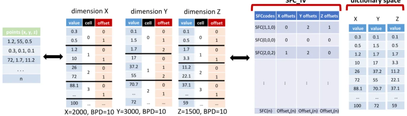
Figure 4: Point cloud data organized according to SFC-DBC Encoding. Improvement over SFC.Compared to traditional SFC-based

approaches, SFC-DBC minimizes storage footprint and increases resilience to skew. SFC-DBC achieves this by constructing a space-filling curve over a reduceddictionary space, instead of the original data space (universe). This partitioning strategy has a twofold ef-fect on SFC-DBC. First, it enables the integration of SFC into the dictionary model. This consequently lowers the storage footprint and assigns two roles to the SFC: the role of spatial index andIV in DBC. Second, it enables a better adjustment ofSFCcodesto the distribution of the data.

Figure 3 illustrates an example of data partitioning using both SFC-DBC and traditional SFC-based strategy. We use the subset of a dataset represented with six points p1-p5 & pn and assume that each dimension is divided into four cells. The SFC order, constructed ac-cording to the traditional encoding scheme, follows space-oriented partitioning, i.e., it uses uniform partitioning of the space, regard-less of data distribution. As opposed to this, SFC order in SFC-DBC is defined in a driven way. As illustrated in the example, data-driven partitioning improves skew handling, since it is done based on the actual points values. Data-partitioning also restricts the number of distinct points per cell, additionally improving skew resilience. In the example, SFC-DBC can have at most four distinct points per cell, while space-oriented partitioning does not have these guaranties.

In the following subsections we discuss necessary data structures and describe how to build and use them in the preprocessing and querying step. Finally, we conclude with the benefits and scope of our approach.

3.1 Preprocessing & Data Structures

The SFC-DBC approach represents a point cloud entry through its position in an artificially introduced 3Ddictionary spaceand indexes it using a SFC order. Consequently, the preprocessing step results in two types of data structures: dictionary- and index-like structures. In the following we describe these structures and the preprocessing step that produces them.

Data Structures.SFC-DBC operates on adictionary spaceand aspace-filling curve index vector (SFC_IV) data structures, as il-lustrated in Figure 2 and Figure 4. Thedictionary spaceis a 3-dimensional space reconstructed fromx,y, andzdictionaries that captures the distinct values of point cloud entries in each dimension.

SFC_IVmaps each point to its position in thedictionary spaceand thereby its value. At the same time, it plays the role of a spatial index by encoding the point through its position in the SFC order constructed on top of thedictionary space.

To uniquely identify the position of a point indictionary space, SFC_IV further consists of theSFCcodesandoffsetsvectors. The SFCcodesvector maps the point to its position in the SFC order based on the assignedSFCcode. The correspondingSFCcodedoes not uniquely identify the position of the point in thedictionary space but rather the cell it is in, as we assume that a point cloud entry does not have a unique representation in the SFC order. Therefore, we additionally capture the position of the point within the cell using theoffsetsvector data structure. TheSFCcodesstructure is ad-ditionally compressed to minimize the storage requirements. More precisely, considering that multiple points map to the sameSFCcode, we store just the distinctSFCcodesvalues and their corresponding starting positions in the input.

Preprocessing.The preprocessing step consists of four tasks

that we describe through an example illustrated in Figure 4. First, we begin by producing a 3Ddictionary spaceand a grid on top of it. More precisely, we produce a dictionary per dimension and divide them into cells, for each dimension independently. The number of cells is determined by the number of bits assigned per dimension (BPD) in theSFCcodeand it corresponds to2BPD. For instance, in the example (Figure 4), thexdictionary is divided into 1024 cells as BPD corresponds to 10. Consequently, every cell has two dictionary entries, given that the number of entries in thexdictionary is 2000. Notice that the number of entries per cell (EPC) differs betweenx,y, andzdimensions as the dictionaries have different sizes (depending on the number of distinct values per dimension).

Second, once thedictionary spaceis partitioned, we assign a SFC-codeto every point according to the dictionary cells they belong to. For instance, the first pointP(1.2,55,0.5)in the example (Figure 4, points) belongs to the cells with ids 1, 1 and 0 for thex,y, andz dimension respectively, and thus theSFCcodeencodes these ids. The ids, however, do not uniquely identify the position of the point in the dictionaries. To do so, in the third step we additionally store the position of the point within the cells (Figure 4,offsets) – therefore, for the first point we store 0, 2 and 1 values according tox,y, andz dimensions. Lastly, once the final structures are produced, we sort them according to the assignedSFCcode.

(5)

Algorithm 1:Query Execution: produce candidate results set Input:q: range query - defined with two coordinates Output:minDQ, maxDQ: min and max position in dictionary

that corresponds to query range

Output:candidateSet: candidate result set

//transforms query to 1D:

ford=0todimensionsdo

minDQ[d]=binaryS(dictionary[d],q.low[d]) maxDQ[d]=binaryS(dictionary[d],q.hiдh[d])

end

qSFCcodes=calcSFCcode(q,minDQ,maxDQ) candidateSet=binaryS(qSFCcodes,SFCcodes)

returncandidateSet

3.2 Query Execution

Similar to the traditional SFC-based approach, the query execution is composed of two steps. In the first step, theSFCcodesvector restricts search space by producing the candidate results set, while in the second step we additionally prune, i.e., remove false positive results.

The first step is illustrated in Algorithm 1. The query execution first transforms the query range to the 1D domain, by determining its position in thedictionary spaceand calculating the correspond-ingqSFCcodes. Based on the produced codes, we determine the candidate result set by performing binary search on theSFCcodes vector. The resulting candidate set may contain false positive re-sults considering that theSFCcodeis assigned per cell and not per point. Therefore, in the second step we check if the identified points indeed belong to the query range.

To do so, we reconstruct the position of the point in the dictio-nary (and thus its value) for the points identified in the candidate results set and check if they belong to the query range. We perform this algorithm for all three dimensions in parallel, as illustrated in Algorithm 2. More precisely, the position is reconstructed by combining the decodedSFCcodeandoffsetvalues, i.e., applying the following formula for the corresponding dimension:

position=cell_id×#EPC+of f sets (1)

wherecell_idrepresents the dictionary cell id obtained by decod-ing theSFCcodefor the corresponding dimension andEPCstands for the number of entries per cell in the corresponding dictionary. Once the position is reconstructed, we check if it belongs to the query range <minDQ,maxDQ>, which corresponds to the mini-mum and maximini-mum position in the dictionary that the query maps to (obtained in Algorithm 1).

Filtering.The time consuming operations in this process are

the scan of theoffsetsvector and the decoding of theSFCcode. As the decoding is done once per distinctSFCcodevalue (once a value is decoded it is reused for all the points that have the sameSFCcode), the scan of theoffsetsvector dominates the total execution time, as illustrated in Section 4.2. Therefore, to optimize theoffsetsvector scan, SFC-DBC minimizes the number of the offset entries neces-sary to be examined by skipping the entries that are completely enclosed by the query range. This can be done by checking the enclosedByQuerycondition in Algorithm 2, which requires just the decodedSFCcodeandEPCvalues in order to calculate the minimum

Algorithm 2:Query Execution: produce final results set Input:q: range query - defined with two coordinates Input:candidateSet: candidate result set

Input:minDQ, maxDQ: min and max position in dictionary

that corresponds to query range

Input:EPC: number of entries per cell, d - dimension Output:pOut: point cloud result set

fori=value incandidateSetdo cell_id=decode(SFCCodes[i],d) base=cell_id∗EPC[d]

//retrieve the positions of the points for the given SFCcode <inputMin, inputMax> = mapSFCcodeToInputPosition(i) //enclosedByQuery condition

ifminDQ[d]<baseAND(base+EPC[d])<maxDQ[d]

then

pOut.setRanдe(inputMin,inputMax) continue

end

//not enclosedByQuery - retrieve offsets

forj=inputMin;j<inputMaxdo

position = base + offests[j];

ifminDQ<position<maxDQthen pOut.set(j)

end end end returnpOut

and maximum position in dictionary that the points with a given SFCcodecan map to. Intuitively, this optimization is more beneficial for the non-selective queries, as illustrated in Section 4.5.

3.3 Discussion

SFC-DBC enhances dictionary-based compression with indexing capabilities, optimizing for query execution without introducing additional space requirements. Therefore, in the following we ana-lyze the space requirements of the baseline DBC and SFC-DBC. We conclude the section discussing the scope of our approach.

3×(DS×de+n×loд₂DS) (2)

Space Requirements.As illustrated in Section 2.1, the baseline

DBC operates based ondictionariesandIV. Therefore, its total space requirements correspond to Equation 2, where for the sake of simplicity we assume that each dictionary in 3D space has the same length. More precisely, 3×DS×derepresents the space requirements

of thedictionaries, whereDSanddeare the number of entries and the size of an entry in the corresponding dictionary respectively. IVscorresponds to 3×n×loд₂DS, wherenis the number of points andloд₂DSis the number of bits perIVentry (which corresponds to the number of bits necessary to represent the maximum position in the corresponding dictionary).

On the other hand, the SFC-DBC approach storesdictionaries, off-setsandSFCcodesvectors, resulting in the total space requirements illustrated in Equation 3. More precisely, thedictionariesare repre-sented with 3×DS×de, theoffsetsvectors with 3×n×loд₂⌈DS/2BP D⌉

(6)

SFCcodesvector corresponds to #SFCcode×3×BPDwhere

#SFC-code represents the number of distinctSFCcodevalues. Compared to the space requirements of the baseline DBC – thedictionariesare identical,offsetsvector minimizes the resources ofIVsince an offset entry indexes the values within a dictionary cell as opposed to the entire dictionary, whileSFCcodesvector introduces additional space requirements.

3×(DS×de+n×loд₂⌈DS/2BP D⌉+#SFCcode×BPD)

≡3×(DS×de+n×loд₂DS−n×BPD+#SFCcode×BPD) (3) Therefore, comparing the requirements of both approaches (ac-cording to Equation 2 and Equation 3), the SFC-DBC approach subtracts 3×n×BPD, while at the same time it introduces an

addi-tional overhead in the form of 3×#SFCcode×BPD. Considering

thatn ⩾#SFCcode, the benefit is higher than the overhead and thus, the space requirements of SFC-DBC are always smaller or equal to the requirements of DBC.

Scope.As discussed, DBC is a good approach for point cloud

data representation, because of the repetition of values for thex,y, andzcoordinates. A limitation for such dictionary-based solutions is that this property cannot be guaranteed for raw (unprocessed) point cloud data obtained through LiDAR technology, as it results in unstructured form. However, LiDAR data typically obtains these characteristics as the result of post-processing steps (e.g., thinning-out of data) [25, 30].

Additionally, our solution is primarily designed for a static use case, due to the static nature of point cloud data. An insertion/update into our encoding scheme is a possible, yet costly operation as the whole preprocessing might need to be redone. However, this limi-tation does not hurt this scheme in the context of SAP HANA. As we discuss in section 4, HANA has segments of storage that do not need to provide cheap single-insert or update operations due to the Delta/Main concept.

4 EXPERIMENTAL EVALUATION

In this section we first describe the experimental setup and method-ology and then evaluate the performance of the proposed approaches over real-world datasets.

Hardware Configuration.We run experiments on a SuSE Linux

Enterprise Server 12 SP1 machine equipped with 4 Intel Xeon CPU E7-4880v2 processors at 2.50GHz and 512GB of RAM. Each proces-sor has 15 cores with private L1 (32KB) and L2 (256KB) caches, as well as 37,5MB of shared L3 cache.

SAP HANA.HANA is an in-memory database that offers the

pos-sibility to store data in either a row-oriented or a column-oriented fashion. It has a unique way of handling inserts and updates. More precisely, each column partition has two segments, a read-optimized Main segment and a write-optimized Delta segment. Updates and inserts are written to the Delta segment, while Main segments are created by an asynchronous background task. As this process has access to all the column fragment’s data, it can make an optimal decision on the type of the Main segment (such as our SFC-DBC container) to be created and its properties. The column store’s de-sign is centered around SIMD operations to speed up scans of vector data [31]. This design choice is reflected in our proposed encoding scheme. It is necessary to notice that SAP HANA is the system that we used as a proof of concept to develop and evaluate our approach,

however, the proposed solution can be integrated in other main memory column-store DBMS.

Implementation.All indexing techniques are implemented in

C++ and compiled withGCC 4.8.5. The list below summarizes the

implementations that we study experimentally.

Baselinecorresponds to the baseline dictionary-based

compres-sion approach described in Section 2.1.

SFC-DBCrepresents our approach, introduced in Section 3. We

use the Z-order as a SFC order, due to its simplicity and the huge body of work on its efficient range query algorithms (e.g., [2, 27, 28]). In our approach, azcodeencodes the cell ids (forx,y, and zdimension) that a point cloud entry maps to in a uniform grid built over thedictionary spaceand, therefore, we represent azcode as an integer. TheBPDin azcodedetermines the total number of cells (per corresponding dimension) in the uniform grid and, consequently, the maximum number of point cloud entries that can qualify for the second step in the query execution of our approach, i.e., removing false positives. We representzcodewith 32 bits (10 bits per dimension —BPD) as a trade-off between memory resources and precision (number of false positives to be filtered).

SFCstands for the Space-Filling Curve-based approach, which

we implemented as a middle ground solution between the Base-line approach and SFC-DBC. The SFC approach does not require decoding ofSFCcode, however, it needs additional space for its stor-age. Therefore, we use SFC to evaluate SFC-DBC: the overhead introduced with its decoding step, but also the storage benefits.

More precisely, the SFC approach corresponds to the traditional approach described in Section 2.2 with one modification. To have a fair comparison in terms of space requirements, we build a SFC order as an addition to the DBC model. Therefore, the SFC ap-proach extends the Baseline apap-proach with a SFC order, using space-oriented partitioning of the dataset universe. Consequently, it stores theSFCcodesvector in addition to the structures used in the Baseline approach ( Section 2.1). Like in the SFC-DBC approach, we use the Z-order and compress theSFCcodes, each represented with 32 bits. The query execution is adjusted to the DBC model. We first execute a query on theSFCcodesproducing acandidate results set, while in the second step we remove false positive results by examining the actual points. Similar to the Baseline approach, the points are examined by combining the information from dictionar-iesandIVs. However, the scan ofIVis restricted, as we examine just the ranges detected by thecandidate results set.

Datasets. We use two types of datasets, obtained using dense

image matching and LiDAR technologies. "Senatsverwaltung für Wirtschaft, Technologie und Forschung" and "Europäischer Fonds für regionale Entwicklung (EFRE)" provided the datasets that are generated using dense image matching. Berlin aerial scan has reg-ular point distribution with 100 points per square meter, while terrestrial castle scan represents irregular point distribution and a varying point density. We also use AHN2 dataset [18], obtained using LiDAR technology. To evaluate the scalability of approaches, we sample the datasets uniformly, increasing the dataset size from 125 million points to 1 billion points.

Queries.We produce one hundred 2D and 3D range queries that

follow uniform distribution. We vary selectivity by increasing the queries’ volume: 10−2_{%, 10}−1_{%, 1%, 10%, 20%, and 40%.}

(7)

0 2 4 6 8 10 125 250 500 1000 Re la tiv e sp ac e re qu ire m en ts

a) #points in datasets (millions) SFC-DBC Baseline SFC Uncompressed 0 1 2 3 4 SFC -DB C Ba se lin e SFC SFC -DB C Ba se lin e SFC 125 1000 Re la tiv e sp ac e re qu ire m en ts

b) #points in datasets (millions) Dictionary

SFCCode Index

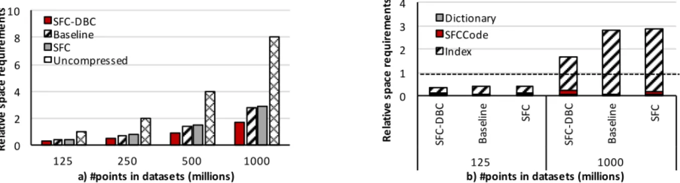
Figure 5: Berlin aerial dataset, space requirements: a) total and b) breakdown.

a) #points in datasets (millions) SFC-DBC Baseline SFC Uncompressed 0 2 4 6 8 10 0 200 400 600 800 1000 Re la tiv e ex ec ut io n tim e

b) #points in datasets (millions)

Baseline SFC SFC-DBC

Figure 6: AHN2 dataset: a) space requirements and b) query execution time (3D queries).

Experimental Results.In all the experiments we illustrate

rela-tive numbers. More precisely, the execution time is relarela-tive to the Baseline approach, i.e., its execution time obtained when process-ing the smallest dataset (125M elements). Followprocess-ing the same logic, the space requirements results are relative to the Uncompressed storage model (considering the smallest dataset).

4.1 Space Requirements

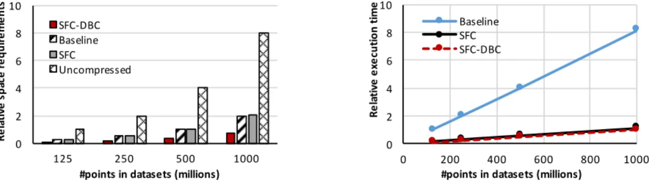
In this set of experiments we evaluate the space requirements of the aforementioned approaches when processing the Berlin aerial and AHN2 datasets. We measure the requirements ofdictionariesand IVsfor the Baseline approach, considering additionally the size of SFCcodesfor the SFC-based approaches. Furthermore, we measure the size of uncompressed data, i.e., when using a straightforward approach of storing all three coordinates. Figure 5a) presents the rel-ative space requirements, while Figure 5b) illustrates the breakdown for the smallest and the biggest point cloud size when processing the Berlin aerial dataset. The horizontal line corresponds to the requirements of the Uncompressed model, for the smallest dataset. Dictionary-based compression significantly reduces the space requirements: the Baseline approach reduces the space necessary to represent uncompressed data by up to 65%. SFC-DBC additionally minimizes the requirements, reducing the Baseline approach stor-age footprint by up to 40%. On the other hand, the SFC approach requires up to 13% more storage compared to the Baseline approach. The observed trends are similar for the AHN2 dataset, as illustrated in Figure 6a).

According to Figure 5b) all dictionary-based approaches have dictionaries of the same size, while the Index (i.e.,IV/offsets) and the SFCcodesrequirements vary. SFC-DBC has the smallest Index size, where the space reduction over the SFC and Baseline approaches is constant - 46%. On the other hand, it produces more distinct SFCcodesvalues compared to the SFC approach due to data-oriented partitioning (as discussed in Section 3). Consequently, it increases the space quota, but it also improves skew handling by enabling a better adjustment ofSFCcodesto the distribution of the data.

4.2 Query Performance

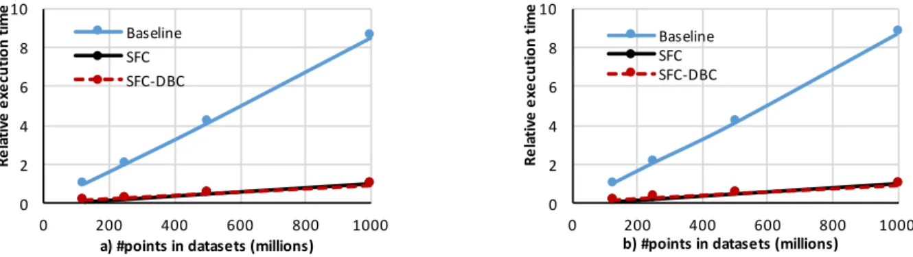
To experimentally evaluate the query performance of SFC-DBC we execute 100 uniformly distributed 3D and 2D range queries with a selectivity of 1% on the Berlin aerial and AHN2 datasets.

Figure 7 illustrates the relative execution time when executing 3D and 2D queries on the Berlin aerial dataset. As the experiment il-lustrates, the Baseline approach requires substantially more time be-cause it scans the completeIVs, whereas the SFC-based approaches scan just the intervals detected by the candidate result set. There-fore, the SFC-DBC approach outperforms the Baseline approach with speedup of 7.5 - 8.9 and 6.8 - 9.4x, when executing 3D and 2D queries respectively. SFC-DBC achieves performance comparable to that of the SFC approach considering that 1) decoding is done once per distinctSFCcodevalue, and 2) the decoded value was suffi-cient to decide whether a point satisfies a range query for 86% of the candidate result set values (i.e., the filtering step was applied, Section 3.2). Therefore, SFC-DBC compensates for the decoding

(8)

0 2 4 6 8 10 0 200 400 600 800 1000 Re la tiv e ex ec ut io n tim e

a) #points in datasets (millions) Baseline SFC SFC-DBC 0 2 4 6 8 10 0 200 400 600 800 1000 Re la tiv e ex ec ut io n tim e

b) #points in datasets (millions)

Baseline SFC SFC-DBC

Figure 7: Berlin aerial dataset, query execution time: a) 3D and b) 2D range queries.

0 0.2 0.4 0.6 0.8 1 1.2 125 1000 Re la tiv e ex ec ut io n tim e

#points in datasets (millions)

Decoding Binary Search&Scan

Figure 8: SFC-DBC: execution time breakdown.

step by its ability to avoid theoffsetsvector scan. The observed trends are similar for the AHN2 dataset, as illustrated in Figure 6b). Figure 8 presents the execution time breakdown for the SFC-DBC approach when processing the smallest and the biggest point cloud datasets. Decoding represents the time necessary to perform decoding ofSFCcodeand the Binary Search&Scan measures the time necessary to perform binary search (onSFCcodesanddictionaries) and the scan of the correspondingoffsets. As the small dataset (125M points) is produced by uniformly sampling the biggest dataset (1000M points), the number of distinctSFCcodevalues does not differ significantly between two datasets – the 1000M dataset has x1.32 more distinctSFCcodes. Therefore, the decoding time takes 71% and 13% of the total execution time, since the number of distinct SFCcodescorresponds to 29% and 5% of the point cloud entries in the smallest and biggest datasets respectively.

4.3 Impact of Skew

In the following set of experiments we analyze the impact of skew on the space requirements and query performance of SFC-based approaches. We execute 100 uniformly distributed 3D queries (1% selectivity) on the Terrestrial castle scan that has irregular point distribution and a varying point density. Figure 9a) measures space requirements, while Figure 9b) illustrates the execution time.

Due to skew in data distribution and density, the space require-ments of the dictionary-based approaches are minimized compared to their requirements when processing data with uniform distribu-tion (Secdistribu-tion 4.1). As the number of distinct values per coordinate decreases, the space requirements ofdictionariesandIVs/offsetsalso

decrease and therefore, the Baseline approach reduces the space necessary to represent uncompressed data by up to 75%. Skew addi-tionally reduces the number of distinctSFCcodesand thus, SFC-DBC reduces the Baseline approach storage footprint by up to 61%.

On the other hand, skew in data distribution and density reflects toSFCcodesdistribution and thus penalizes query performance. More specifically, having fewer distinctSFCcodesincreases the num-ber of point cloud entries needed to be checked for intersection per SFCcode. Therefore, the speedup of SFC-DBC and SFC approaches over the Baseline approach drops up to 10% and 16% compared to the speedup achieved when processing the data with uniform distribution. SFC-DBC incurs smaller performance penalties as the decrease in the number of distinctSFCcodeshas a twofold effect on performance. On one hand, it hurts performance since the number of points necessary to be scanned increases. On the other hand, it decreases the number ofSFCcodesnecessary to be decoded.

4.4 Impact of Selectivity

To evaluate the impact of selectivity on query performance we execute one hundred 3D queries on the Berlin aerial dataset (500 million points) varying selectivity from 10−2_{% to 40%. Figure 10} illustrates the total execution time.

As expected, SFC-based approaches benefit from queries with high selectivity. They minimize the number ofIV/offsetsentries necessary to be scanned using a SFC order as an index, while the Baseline approach performs a fullIVscan. On the other hand, less selective queries (e.g., 40% selectivity) favour the Baseline approach considering that they touch significant amount of data. Thus, the speedup of the SFC-DBC approach drops from 8.4x to 2.8x when decreasing query selectivity.

4.5 Impact of Filtering

To evaluate the impact of filtering (introduced in Section 3.2) on the performance of SFC-DBC, we execute one hundred 3D queries on the Berlin aerial dataset (500 million points) varying selectivity from 10−2_{% to 10%. Figure 11 illustrates the relative execution time} for the SFC-DBC approach, when we enable and disable filtering.

The filtering step minimizes the range that has to be scanned in theoffsetsvector. Since the length of the range is determined by the query selectivity, the impact of filtering depends on the selectivity.

(9)

#points in datasets (millions)

SFC-DBC Baseline SFC Uncompressed 0 2 4 6 8 10 0 200 400 600 800 1000 Re la tiv e ex ec ut io n tim e

#points in datasets (millions) Baseline

SFC SFC-DBC

Figure 9: The impact of skew: space requirements and query execution time.

0 0.5 1 1.5 2 0.01 0.1 1 10 20 40 Re la tiv e ex ec ut io n tim e Query selectivity Baseline SFC SFC-DBC

Figure 10: Execution time when varying query selectivity.

As illustrated in the Figure 11, the filtering step significantly im-proves the execution time for low selectivity queries, considering that it filters more data (e.g., the improvement in the execution time is 38% for 10% selectivity). On the other hand, filtering does not have a significant impact on performance when executing high se-lectivity queries (e.g., for 10−2_{% selectivity queries the improvement} in the execution time is 0.6%).

5 RELATED WORK

In this section we first give a general overview of existing point cloud management systems, following up with compression and indexing capabilities of current systems.

General.File-based solutions (e.g., LAStools [23]) represent a

traditional approach to point cloud data management: points are stored in files in a predefined format and processed by application-specific algorithms. The typical file format is LAS, alongside with compressed alternatives, e.g., Rapidlasso’s LAZ [24] and ESRI’s ZLAS. File-based solutions have been widely used, however, as point cloud data increases in size and popularity, it becomes more challenging for them to fulfill recent data management require-ments. First, file-based solutions have limited functionality in terms of declarative power and multi-user support [29]. Second, they face scalability problems with respect to the increasing number of files to process and their size [1, 29]. A recent benchmark [29] proposes a hybrid solution to address the scalability problem, employing a DBMS to manage the meta-data of a file-based solution.

0 0.5 1 1.5 2 2.5 0.01 1 10 Re la tiv e ex ec ut io n tim e Query selectivity Filtering No Filtering

Figure 11: SFC-DBC: impact of filtering.

Research in this area has recently shifted towards DBMS as many of the data management challenges, encountered with the increas-ing point cloud data size, have already been addressed in DBMS solutions. Current DBMSs support point cloud data management in the form of extensions and specific data types, distinguishing between blocks and the flat table model. The blocks model groups spatially collocated points into blocks, preserving spatial proximity. Although the blocks organization offers basic compression capa-bilities, it also requires blocks to be unpacked when executing queries. This introduces significant overhead when executing high selectivity queries [29]. On the other hand, the flat model uses the straightforward approach of storing one point per row, which makes it efficient when executing less complex queries, however, it requires significant storage resources [29]. A recent benchmark [29] evaluates the performance of these models, experimenting with various systems, including both file-based solutions and DBMSs. More precisely, the blocks storage model was tested through Oracle and PostgreSQL (their point cloud extensions [19, 22]), while the flat model was used in MonetDB, but also in Oracle and PostgreSQL. Recent work [1, 12, 29] illustrates the potential of column-store DBMSs to meet point cloud management requirements. The Mon-etDB demo [1] showcases the declarative power of DBMS when managing point cloud data that is enriched with semantics from different sources. The solution proposed in [12] focuses on imple-mentation details of existing algorithms for spatial selections and joins on modern hardware, and does not address space efficiency.

Compression.The blocks model offers basic compression

(10)

instance, PostgreSQL and LAS take advantage of this by represent-ing the point cloud entries within each block as 32 bit integers with a scale and offset value. An alternative option in PostgreSQL is dimensional compression where each dimension is separately com-pressed using algorithms such as run-length encoding. In [15], the authors propose a compression scheme for the flat storage model in MonetDB. Morton-replacedXY [15] compresses data by repre-senting a point with azcoordinate and Morton code that replaces thexandycoordinates.

Indexing.Both file-based solutions and DBMSs (based on the

blocks model) by default organize data to preserve spatial prox-imity information and thus optimize query execution. This has been mostly done by using space-filling curves, such as the Hilbert curve [10] and the Z-order [20]. To further optimize performance, they use various spatial index structures such as R-Tree [7], oc-tree [9], quadoc-tree [26] etc. The flat model does not preserve spa-tial data properties by default, as it stores thex,y, andz coor-dinates independently. Therefore, one option is to treat data as non-spatial and thus use indexes not tailored to spatial data, such as a B+-Tree [29]. The alternative is to organize data to preserve spatial proximity information, which has been explored both in MonetDB [15] and PostreSQL [29] by using the Morton order.

The majority of the proposed solutions are traditional spatial index structures built in addition to the data model. Therefore, they require additional space resources which can introduce signif-icant overhead, particularly for solutions based on the flat storage model [29]. An exception is the previously introduced Morton-replacedXY approach [15]. However, although the proposed solu-tion integrates Morton order into the flat model, it still requires significant space resources, as Morton code andzvalue are stored per point cloud entry.

6 CONCLUSIONS

With the recent increase in the volume of point cloud data produced, existing data management solutions face two challenges: time and space efficiency. In this work we investigate how the efficiency requirements can be met in main memory column-store DBMSs.

We propose Space-Filling Curve Dictionary-Based Compression (SFC-DBC), a time and space-efficient solution to storing and man-aging point cloud data. Our solution employs dictionary-based compression in the spatial data management domain, enhancing it with indexing capabilities without introducing additional storage overhead. The SFC-DBC approach represents and indexes a point cloud entry through its position in an artificially introduced 3D dictionary space, taking advantage of space-filling curve properties for indexing purposes. We evaluate our approach in the context of SAP HANA and show space efficiency gains of up to 61% and query performance gains of up to 9.4x compared to other dictionary-based compression schemes.

ACKNOWLEDGEMENTS

We would like to thank the reviewers, the DIAS laboratory mem-bers, and Georgios Chatzopoulos for their valuable comments and suggestions on how to improve the paper. We thank "Senatsverwal-tung für Wirtschaft, Technologie und Forschung" and "Europäischer Fonds für regionale Entwicklung (EFRE)" for the provided data. This

work is partially funded by the EU FP7 programme (ERC-2013-CoG), Grant No 617508 (ViDa).

REFERENCES

[1] Foteini Alvanaki, Romulo Goncalves, Milena Ivanova, Martin L. Kersten, and Kostis Kyzirakos. 2015. GIS Navigation Boosted by Column Stores.PVLDB8, 12 (2015), 1956–1959.

[2] Rudolf Bayer. 1997. The Universal B-Tree for Multidimensional Indexing: general Concepts. InWWCA. 198–209.

[3] Christos Faloutsos. 1988. Gray Codes for Partial Match and Range Queries.IEEE Trans. Software Eng.14, 10 (1988), 1381–1393.

[4] Christos Faloutsos and Shari Roseman. 1989. Fractals for Secondary Key Retrieval. InPODS. 247–252.

[5] Franz Färber, Norman May, Wolfgang Lehner, Philipp Große, Ingo Müller, Hannes Rauhe, and Jonathan Dees. 2012. The SAP HANA Database – An Architecture Overview.IEEE Data Eng. Bull.35, 1 (2012), 28–33.

[6] Romulo Goncalves, Tom van Tilburg, Kostis Kyzirakos, Foteini Alvanaki, Panagi-otis Koutsourakis, Ben van Werkhoven, and Willem Robert van Hage. 2016. A spatial column-store to triangulate the Netherlands on the fly. InSIGSPATIAL.

80.

[7] Antonin Guttman. 1984. R-trees: a dynamic index structure for spatial searching. InSIGMOD. 47–57.

[8] Norbert Haala. 2011. Multiray photogrammetry and dense image matching. In

Photogrammetric Week, Vol. 11.

[9] Chris L Jackins and Steven L Tanimoto. 1980. Oct-trees and their use in repre-senting three-dimensional objects.Computer Graphics and Image Processing14, 3

(1980), 249–270.

[10] H. V. Jagadish. 1990. Linear Clustering of Objects with Multiple Atributes. In

SIGMOD. 332–342.

[11] Christian S. Jensen, Dan Lin, and Beng Chin Ooi. 2004. Query and Update Efficient B+-Tree Based Indexing of Moving Objects. InPVLDB. 768–779.

[12] Kostis Kyzirakos, Foteini Alvanaki, and Martin L. Kersten. 2016. In memory processing of massive point clouds for multi-core systems. InDaMoN. 7:1–7:10. [13] Per-Åke Larson, Cipri Clinciu, Eric N. Hanson, Artem Oks, Susan L. Price,

Sriku-mar Rangarajan, Aleksandras Surna, and Qingqing Zhou. 2011. SQL server column store indexes. InSIGMOD. 1177–1184.

[14] Robert Laurini. 1985. Graphics databases built on Peano space-filling curves. In

EUROGRAPHICS, Vol. 85.

[15] Oscar Martinez-Rubi, Peter van Oosterom, Romulo Goncalves, Theo Tijssen, Milena Ivanova, Martin L. Kersten, and Foteini Alvanaki. 2014. Benchmarking and improving point cloud data management in MonetDB.SIGSPATIAL Special

6, 2 (2014), 11–18.

[16] Mohamed F. Mokbel and Walid G. Aref. 2009. Space-Filling Curves for Query Processing. InEncyclopedia of Database Systems. 2675–2680.

[17] Bongki Moon, Hosagrahar V Jagadish, Christos Faloutsos, and Joel H Saltz. 2001. Analysis of the clustering properties of the Hilbert space-filling curve.TKDE13,

1 (2001), 124–141.

[18] Actueel Hoogte Bestand Nederland. 2017.AHN datasets. http://www.ahn.nl.

[19] Oracle. 2017. Spatial and Graph Developer’s Guide. https://docs.oracle.com/

database/121/SPATL/.

[20] Jack A Orenstein and Tim H Merrett. 1984. A class of data structures for associa-tive searching. InPODS. 181–190.

[21] Giuseppe Peano. 1890. Sur une courbe, qui remplit toute une aire plane. In

Mathematische Annalen. 157–160.

[22] PostgreSQL. 2017.A PostgreSQL extension for storing point cloud (LiDAR) data.

https://github.com/pgpointcloud/pointcloud.

[23] rapidlasso GmbH. 2017.LAStools. https://rapidlasso.com/lastools/.

[24] rapidlasso GmbH. 2017.LAZ format. https://rapidlasso.com/category/laz/.

[25] Rico Richter and Jürgen Döllner. 2010. Out-of-core real-time visualization of massive 3D point clouds. InAfrigraph. 121–128.

[26] Hanan Samet. 1984. The Quadtree and Related Hierarchical Data Structures.

CSUR16, 2 (1984), 187–260.

[27] Tomás Skopal, Michal Krátký, Jaroslav Pokorný, and Václav Snásel. 2006. A new range query algorithm for Universal B-trees.Information Systems31, 6 (2006), 489–511.

[28] Herbert Tropf and H Herzog. 1981. Multidimensional Range Search in Dynami-cally Balanced Trees.ANGEWANDTE INFO.2 (1981), 71–77.

[29] Peter van Oosterom, Oscar Martinez-Rubi, Milena Ivanova, Mike Hörhammer, Daniel Geringer, Siva Ravada, Theo Tijssen, Martin Kodde, and Romulo Goncalves. 2015. Massive point cloud data management: Design, implementation and execu-tion of a point cloud benchmark.Computers & Graphics49 (2015), 92–125.

[30] Aloysius Wehr and Uwe Lohr. 1999. Airborne laser scanning - an introduction and overview.P&RS54, 2 (1999), 68–82.

[31] Thomas Willhalm, Nicolae Popovici, Yazan Boshmaf, Hasso Plattner, Alexander Zeier, and Jan Schaffner. 2009. SIMD-Scan: Ultra Fast in-Memory Table Scan using on-Chip Vector Processing Units.PVLDB2, 1 (2009), 385–394.