binaural cues using temporal context and
convolutional neural networks
Alfredo Zermini, Qiuqiang Kong, Yong Xu, Mark D. Plumbley, Wenwu Wang Centre for Vision, Speech and Signal Processing, University of Surrey
Guildford, Surrey, GU2 7XH, UK
{a.zermini,q.kong,yong.xu,m.plumbley,w.wang}@surrey.ac.uk
Abstract. Given binaural features as input, such as interaural level dif-ference and interaural phase difdif-ference, Deep Neural Networks (DNNs) have been recently used to localize sound sources in a mixture of speech signals and/or noise, and to create time-frequency masks for the esti-mation of the sound sources in reverberant rooms. Here, we explore a more advanced system, where feed-forward DNNs are replaced by Con-volutional Neural Networks (CNNs). In addition, the adjacent frames of each time frame (occurring before and after this frame) are used to exploit contextual information, thus improving the localization and sep-aration for each source. The quality of the sepsep-aration results is evaluated in terms of Signal to Distortion Ratio (SDR).
Keywords: convolutional neural networks, binaural cues, reverberant rooms, speech separation, contextual information
1
Introduction
Sound source separation has been studied for a long time, with implement-ing methodologies such as independent component analysis [1], computational auditory scene analysis [2], and non-negative matrix factorization [3]. More re-cently, Deep Neural Networks (DNNs) [4] and Convolutional Neural Networks (CNNs) [5] have shown state-of-the-art performance in source separation [6–8]. This paper studies the problem of separating two speakers in rooms with differ-ent reverberation, which is a common scenario in real life. A target speech signal, corresponding to the main speaker, is disturbed by an interferer speaker, located in variable positions. This problem has already been studied in [8], where the target speech is separated by generating a time-frequency (T-F) mask, which is obtained by training a DNN by using binaural spatial cues such as mixing vectors (MV), interaural level difference (ILD) and interaural phase difference (IPD). The methods have limitations for more reverberant rooms, in particular when the training room used is different from the room used in the testing set. In recent years, different types of approaches have been developed to overcome these issues. In [9], the introduction of spectral features such as the Log-Power
channels) and contain convolutional and pooling layers [5]. CNNs have been used to estimate the DOA for speech separation in [12] and trained using synthesized noise signals, but recorded with a four-microphones array.
In this paper, we present a system that is able to perform source localization and source separation. Here, the relatively simple system of DNNs already intro-duced by Yu et al. in [8] is upgraded to a deeper system based on CNNs, in order to exploit the increased computational power available in modern GPUs, aiming for a better separation quality. In addition, contextual frame expanding [10] is introduced, which uses the information from neighbouring time frames before and after a given time frame. This gives a better estimation of each T-F point of the soft-mask because the DOA is estimated by checking if a speaker is still active in the time frames around the one that has been estimated.
The remainder of the paper is organized as follows. Section 2 introduces the pro-posed method, including the overall CNN architecture employed, the low-level feature extraction for the CNN input, and the output in the training stage and the system implementation. Section 3 describes how the soft-masks are gener-ated starting from the output of each CNN. Experimental results are presented in Section 4, where evaluations are performed and analyses are given, followed by conclusions of our findings and insights for future work in Section 5.
2
Proposed Method
2.1 System overview
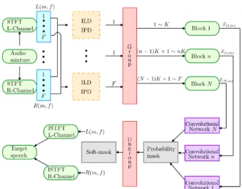
A system of CNNs, shown in Figure 1, is used to localize the direction of one or more speakers in a speech mixture. This system integrates the information from several CNNs, each one trained with the information from a narrow fre-quency band. The outputs are then merged together to get soft-masks, which are used to retrieve the speech source from the audio mixture, as shown in Figure 1. The Short-Time Fourier Transform (STFT) on the left and right channels is calculated. The results are two spectrogramsXL(m, f)andXR(m, f), where
m= 1,· · · , M and f = 1,· · ·, F are the time frame and frequency bin indices respectively. For each T-F point, low-level features (i.e. ILD and IPD) are cal-culated and used to train the CNNs. These features will be introduced in more detail in Section 2.2. The low-level features are arranged intoN blocks, each one containing the information from a small group of frequency bins and the output is a probability mask containing the information from just a narrow frequency band. Each of theN = 128blocks, labelledn, includesK= 8frequency bins in the range ((n−1)K+ 1,· · · , nK), small enough to reduce losses in resolution
Figure 1: Diagram of the system architecture using CNNs.
in the resulting probability output mask, whereK=F/N andN is the number of CNNs. Each block is used as the input of a different CNN for the training stage, each output is a softmax classifier, which gives the probability for a sound source to come from one of the possibleJ DOAs, so it containsJ values between 0 and 1. As explained in section 3, a series of soft-masks can be generated by stacking all the CNNs outputs, one for each test setj and by ungrouping each block into8frequency bins. The binaural soft-masks are multiplied element-wise by the mixture spectrograms and, after applying the inverse STFT (ISTFT), the target source can be recovered.
2.2 Low-level features
The binaural features used are IPD and ILD, have been already introduced for sound localization in [9] [10]. They are used to derive high-level features which are easy to classify. IPD and ILD are the phase and the amplitude difference between the left and the right channels. By putting them in one vector, one can obtain, for each T-F unit:
x(m, f) = [ILD(m, f), IP D(m, f)]T.
Eachu˜(m, f)is grouped intoN blocks along the frequency bins, which represents the input vector of each CNN:
x(n,m)=
xT(m,(n−1)K+ 1),· · ·,xT(m, nK)T.
3
Soft-masks construction
An output mask is created by exploiting the contextual time frame information from the neighbouring frames. A number of time frames τ is selected before
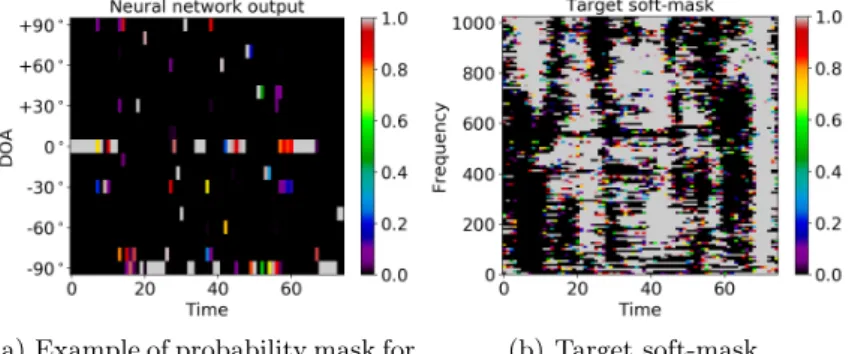
probability as a function of the time frame. By averaging over all the time frames and the frequency bands, the highest value indicates the most probable DOA. The next step is selecting the entire row corresponding to the highest DOA probability. This row represents the target soft-mask for that specific frequency band. As last step, all the probability masks are stacked in order to build the T-F soft-mask for the target speech, shown in Figure 2(b).
(a) Example of probability mask for one of the128CNNs.
(b) Target soft-mask.
Figure 2: Probability mask and soft-mask.
4
Experiments
4.1 Experimental setup
Binaural audio recordings are created by convolving a speech recording with Binaural Room Impulse Responses (BRIRs), captured in real echoic rooms [13]. The BRIRs dataset was recorded around a half-circular grid, ranging from−90◦
to 90◦ with steps of 10◦, for a total of J = 19 DOAs. A dummy head located at the center of a given reverberant room has been used, with left and right microphones, as shown in Figure 3. The training set has been produced by using speech samples from the TIMIT dataset, containing recordings of sentences from different male and female speakers, sampled at f s = 16kHz, high enough for our task. The training samples are randomly selected single reverberant speech recordings,8 males and8 female speakers, recorded at19different DOAs, each one being ≈ 2.3 s long. For the testing set, the same experimental setup and parameters as in [8] have been used. Two different speakers, named the target and
Figure 3: The experimental setup.
the interferer, have been randomly selected from the TIMIT database for the two genders and mixed, for a total of15reverberant speech mixtures for each DOA,≈ 2.3slong each. The experimental setup is shown in Figure 3. Both the target and interferer are located 1.5 maway from the dummy head, and the three objects have the same height. The amount of reverberation depends on the parameters of the room selected, listed in Table 1, where room ‘A’ is less reverberant and ‘D’ more reverberant. The STFT is performed where the Hann window is set to2048(128ms) samples with75% overlap between the neighbouring windows, so the resulting training and testing samples are75time frames long each. The
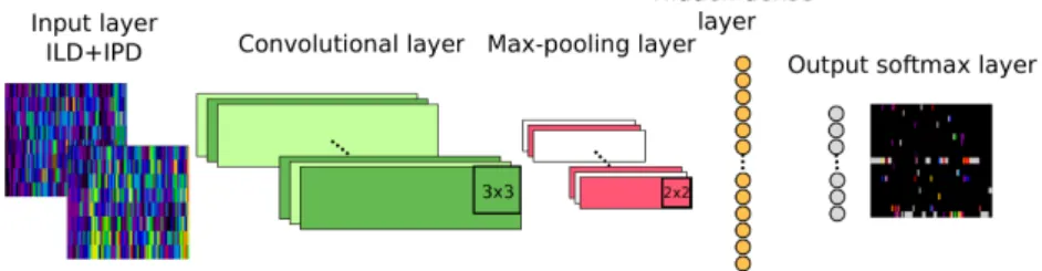
Figure 4: Structure of a CNN.
parameters for each CNN in Figure 4, are found empirically and gave the best performance in our experiments. The first part of the CNN is used for features learning. There is a convolutional input layer with 32feature maps, kernel size (3,3), batch normalization, followed by a max pooling layer with pooling size (2,2) (or (1,1) for τ = 0, to keep the right dimensions) and a 10% dropout layer. The second part is for classification. We used a1024neurons dense layer, with batch normalization and 10% dropout. The output is another dense layer with19neurons. The rectified linear activation function has been used for both the convolutional and the hidden dense layer, while the softmax is used in the output. The number of epochs is set between60 and 200, the batch size is set to200 and the cost-function is the categorical cross-entropy.
Room Type ITDG(ms) DRR(dB)T60(s) A Medium office 8.73 6.09 0.32
D Large seminar room 21.6 6.12 0.89
(a) SDRs evaluation: train room A, test room A, target at0◦.
(b) SDRs evaluation: train room D, test room D, target at0◦.
(c) SDRs evaluation: train room A, test room D, target at0◦.
(d) SDRs evaluation: train room D, test room A, target at0◦. Figure 5: SDR plotted against the DOA, target at0◦.
(a) SDRs evaluation: train room A, test room A, target at−90◦.
(b) SDRs evaluation: train room D, test room D, target at−90◦.
(c) SDRs evaluation: train room A, test room D, target at−90◦.
(d) SDRs evaluation: train room D, test room A, target at−90◦. Figure 6: SDR plotted against the DOA, target at−90◦.
visualization of the plots. When target and interferer are aligned (i.e. from the same direction), it is virtually impossible to separate the two speakers by using spatial features only, so they have been excluded from the plots as well. In Figures 5 and 6, the system named CNNsτ= 0 has been trained and tested without using any contextual information from the neighbouring time frames, while CNNs with τ= 1and τ= 3 includeτ contextual frames before and after each time frame. The last system, named DNNs, is a three dense layers DNNs system, similar to the one tested by Yu et al. in [8], here included as a baseline. The average improvement over all the DOAs compared to the baseline system,
∆SDR, is shown in Table 2.
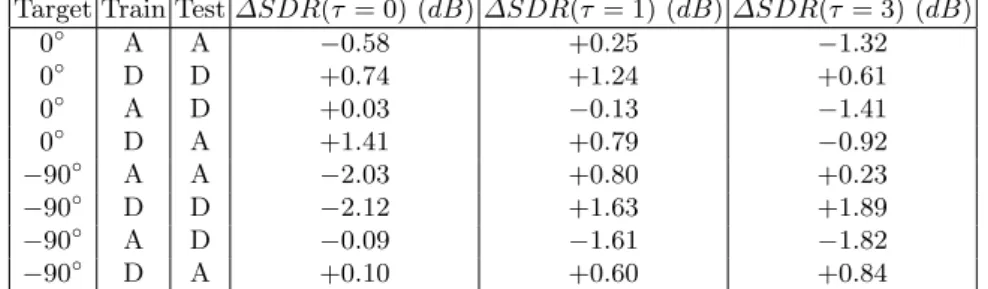
Figures 5(a) and 5(b) show the cases in which the room used for training Target Train Test∆SDR(τ = 0)(dB)∆SDR(τ = 1)(dB)∆SDR(τ= 3)(dB)
0◦ A A −0.58 +0.25 −1.32 0◦ D D +0.74 +1.24 +0.61 0◦ A D +0.03 −0.13 −1.41 0◦ D A +1.41 +0.79 −0.92 −90◦ A A −2.03 +0.80 +0.23 −90◦ D D −2.12 +1.63 +1.89 −90◦ A D −0.09 −1.61 −1.82 −90◦ D A +0.10 +0.60 +0.84
Table 2: Average improvement on the SDRs for the CNNs at differentτcompared to the DNNs baseline.
and testing is the same. For room ‘A’, the CNNs with τ = 1system performs the best among the four systems tested, with ∆SDR ≈ 0.25 dB. The SDRs are in the range ≈ [10,13] dB in Figure 5(a) for τ = 1, giving a very good separation quality on the listening tests. The SDRs decrease while the interferer approaches0◦, because the binaural features contain less information when the differences in level and phase between left and right microphones are small. For room ‘D’, the CNNs withτ = 1 give optimal results, as shown in Figure 5(b), with∆SDR≈1.23dB. The SDRs are in≈[6,10]dB, a good separation quality for a room with such a high reverberation level. The standard deviation, which is on average ≈3dB, highly depends on the gender selection of the mixtures. In fact, where the speech recordings are from speakers of different genders, the frequency overlap is less compared to the case of same gender speakers, which means they are easier for the CNNs to localize.
Figures 5(c) and 5(d) show the cases where the training and testing room do not match. In this case, all the four systems perform slightly worse than the case in which training and testing rooms are the same, as they need to adapt to a type of reverberation that was not included in the training data. Figure 5(c) shows
that DNNs and the CNNs with τ = 0 and τ = 1 have similar performances. Instead, in Figure 5(d), theτ = 0CNNs system has the best separation quality, with ∆SDR ≈1.41 dB. Both in Figure 5(c) and 5(d), the CNNs with τ = 3 give by far the worst performance.
In all the Figures 6 the target is fixed at−90◦. In Figures 6(a) and 6(b), training
and testing rooms are the same. In Figure 6(a) again, the case withτ= 1shows the best performance, with∆SDR≈0.71dBand SDRs in≈[3,6]dB. In Figure 6(b), unlike Figure 6(a), the caseτ= 3performs slightly better thanτ= 1, with
∆SDR≈1.68dBand SDRs in≈[0,3]dB. In both cases,τ= 0gives by far the worst separation results, suggesting that the contextual information improves the system in the localization task, especially in challenging scenarios when the target is located at wide angles. In the cases of room mismatch, plotted in Figures 6(c) and 6(d), all the four systems have difficulty in retrieving the target, with SDRs on average below0 dB.
5
Conclusions and future work
We presented a system of CNNs trained with binaural features and contextual information from the neighbouring time frames, where we used the outputs to build T-F masks. We applied these masks to speech mixtures to retrieve a target speaker. A system with a three dense layers DNNs had already been successfully tested for the same task in [8], showing some limitations, especially when the reverberation time of the testing room is long. As can be seen in Table 2, the sys-tems of DNNs and CNNs with no contextual information, can be considerered complementary, the separation quality depending on the training and testing rooms parameters. In general, when some contextual information is introduced, the CNNs outperform the DNNs baseline. In particular, when a smallτis chosen, optimal results can be obtained, as summarized in Table 2. A possible expla-nation could be that introducing a large amount of contextual frames might include frames belonging to the interferer speaker, resulting in degradation in separation performance. Other works, such as [11], where a DNN is used for speech enhancement, suggest the use of a larger amount of contextual informa-tion, but they show how this is strictly related to the amount of training data, the neural network used and the task at hand. We have also tested the CNNs in more extreme conditions. In particular, when the target is fixed at−90◦, its
contribution arriving at the far-side ear is attenuated as compared to that of the near-side ear, which makes the separation task more challenging. Moreover, testing the networks in mismatched conditions, where the CNNs have to adapt to a new type of reverberation, in addition to the target located at wider angles, is a very challenging scenario, as shown in Figures 6(c) and 6(d). Listening tests indicate that the target source is not separated, suggesting that none of the four systems tested has been effective.
As a future work, we believe that introducing the information from a regression model, along with the classification model presented in this paper, could further improve the separation perfomance, especially in rooms with longer
reverbera-agreement no 607290 SpaRTaN.
References
1. P. Comon and C. Jutten, editors.Handbook of Blind Source Separation : Indepen-dent Component Analysis and Applications. Elsevier, Amsterdam, Boston (Mass.), 2010.
2. D. Wang and G. J. Brown. Computational Auditory Scene Analysis: Principles, Algorithms, and Applications. Wiley-IEEE Press, 2006.
3. D. D. Lee and S. H. Sebastian. Algorithms for non-negative matrix factorization. In T. K. Leen, T.G. Dietterich, and V. Tresp, editors,Advances in Neural Information Processing Systems 13, pages 556–562. MIT Press, 2001.
4. G. E. Hinton and R. R. Salakhutdinov. Reducing the dimensionality of data with neural networks. Science, 313(5786):504–507, July 2006.
5. Y. LeCun, Y. Bengio, and Hinton G. Deep learning. Nature, 521:436, may 2015. 6. Y. Jiang, D. Wang, R. Liu, and Z. Feng. Binaural classification for reverberant
speech segregation using deep neural networks. IEEE/ACM Transactions on Au-dio, Speech & Language Processing, 22(12):2112–2121, December 2014.
7. P.-S. Huang, M. Kim, M. Hasegawa-Johnson, and P. Smaragdis. Joint optimiza-tion of masks and deep recurrent neural networks for monaural source separaoptimiza-tion. IEEE/ACM Transactions on Audio, Speech & Language Processing, 23(12):2136– 2147, December 2015.
8. Y. Yu, W. Wang, and P. Han. Localization based stereo speech source separation using probabilistic time-frequency masking and deep neural networks. EURASIP Journal on Audio, Speech, and Music Processing, 2016(1):7, Mar 2016.
9. A. Zermini, Q. Liu, Y. Xu, M. D. Plumbley, D. Betts, and W. Wang. Binaural and log-power spectra features with deep neural networks for speech-noise separa-tion. In MMSP 2017 - IEEE 19th International Workshop on Multimedia Signal Processing, pages 1–6. IEEE, October 2017.
10. Y. Xu, J. Du, L. Dai, and C. Lee. A regression approach to speech enhancement based on deep neural networks. IEEE/ACM Transactions on Audio, Speech & Language Processing, 23(1):7–19, January 2015.
11. Y. Xu, J. Du, L. R. Dai, and C. H. Lee. An experimental study on speech enhance-ment based on deep neural networks.IEEE Signal Processing Letters, 21(1):65–68, Jan 2014.
12. S Chakrabarty and E. A. P. Habets. Multi-speaker localization using convolutional neural network trained with noise. In 31st Conference on Neural Information Processing Systems (NIPS 2017), 2017.
13. C. Hummersone. A psychoacoustic engineering approach to machine sound source separation in reverberant environments. https://github.com/IoSR-Surrey/ RealRoomBRIRs/, 2011.