Real-Time Prefetching on Shared-Memory Multi-Core Systems

real-time prefetching on

shared-memory multi-core systems

jamie garside

doctor of philosophy university of york

computer science

Abstract

In recent years, there has been a growing trend towards using multi-core pro-cessors in real-time systems to cope with the rising computation requirements of real-time tasks. Coupled with this, the rising memory requirements of these tasks pushes demand beyond what can be provided by small, private on-chip caches, re-quiring the use of larger, slower off-chip memories such as DRAM. Due to the cost, power requirements and complexity of these memories, they are typically shared between all of the tasks within the system.

In order for the execution time of these tasks to be bounded, the response time of the memory and the interference from other tasks also needs to be bounded. While there is a great amount of current research on bounding this interference, one popular method is to effectively partition the available memory bandwidth between the processors in the system. Of course, as the number of processors increases, so does the worst-case blocking, and worst-case blocking times quickly increase with the number of processors.

It is difficult to further optimise the arbitration scheme; instead, this scaling prob-lem needs to be approached from another angle. Prefetching has previously been shown to improve the execution time of tasks by speculatively issuing memory accesses ahead of time for items which may be useful in the near future, although these prefetchers are typically not used in real-time systems due to their unpre-dictable nature. Instead, this work presents a framework by which a prefetcher can be safely used alongside a composable memory arbiter, a predictable prefetch-ing scheme, and finally a method by which this predictable prefetcher can be used to improve the worst-case execution time of a running task.

C O N T E N T S

2 background & related work 31 2.1 Predictability . . . 31

2.1.1 Deriving Predictability Estimates and Bounds . . . 32

2.1.2 Response Time . . . 35

2.1.3 Priority Ceiling Protocol . . . 37

2.2 Memory . . . 38

2.2.1 Predictable DRAM Access . . . 42

2.2.2 Summary . . . 46

2.3 The Move to Multi-Core . . . 47

2.3.1 Memory Arbitration . . . 49

2.3.2 Distributed Memory Arbitration . . . 55

2.3.3 Summary . . . 58 2.4 Prefetching . . . 60 2.4.1 Adaptive Techniques . . . 64 2.4.2 Memory-Side Prefetching . . . 65 2.4.3 Multi-core Prefetch . . . 66 2.4.4 Summary . . . 68 2.5 Summary . . . 68 3 real-time prefetching 71 3.1 Memory Arbitration . . . 72 3.2 Prefetching . . . 74

3.3 Real-Time Prefetching . . . 77

3.3.1 Requesters . . . 79

3.3.2 Arbiter . . . 80

3.3.3 Memory & Memory Controller . . . 81

3.3.4 Prefetcher . . . 82

3.3.5 Discussion . . . 83

4 real-time prefetching on multicore 89 4.1 Introduction . . . 89 4.2 System Architecture . . . 89 4.2.1 Arbitration Scheme . . . 90 4.2.2 Requesters . . . 99 4.2.3 Prefetcher . . . 101 4.2.4 Memory Controller . . . 108 4.3 Evaluation Methodology . . . 109 4.3.1 Hardware Setup . . . 109 4.3.2 Workload Generation . . . 111

4.4 Results - Low Priority Prefetching . . . 112

4.4.1 Worst-Case Conditions . . . 112

4.4.2 Average-Case Conditions . . . 113

4.5 Results - High Priority Prefetching . . . 116

4.5.1 Worst-Case Conditions . . . 117

4.5.2 Average-Case Conditions . . . 124

4.6 Summary . . . 126

5 worst-case aware prefetching 129 5.1 Prefetching Safely . . . 129

5.1.1 Task Model . . . 129

5.1.2 Prefetching Methods . . . 131

5.2 System Design . . . 135

5.2.1 Updated System Model . . . 135

5.2.2 Updated Bluetree Multiplexers . . . 137

5.2.3 Updated Prefetcher . . . 140

5.3 System Evaluation . . . 145

5.3.1 Evaluation Methodology . . . 145

5.3.2 Software Traffic Generators . . . 146

5.3.3 Real-World Benchmarks . . . 150

5.4 Summary . . . 152

6 wcet improving prefetch 153 6.1 Improving the Worst-Case . . . 153

6.1.2 A Better Prefetching Approach . . . 156

6.1.3 Improving the Worst Case . . . 161

6.2 Evaluation . . . 163

6.2.1 Static Analysis . . . 163

6.2.2 Worst-Case Hardware System . . . 166

6.3 Summary . . . 169

7 conclusions and future work 171 7.1 Contributions . . . 171

7.2 Conclusions . . . 172

7.3 Further Work . . . 174

7.4 Closing Remarks . . . 175

L I S T O F F I G U R E S

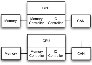
Fig. 1.1 Example multi-CPU system, comprised of two independent CPUs

with private memories. . . 23

Fig. 1.2 Example multi-core system, comprised of a dual-core CPU with a single shared memory. . . 23

Fig. 1.3 Example multi-core system, comprised of a dual-core CPU with a single arbitrated shared memory. . . 25

Fig. 1.4 The growing gap between CPU and memory performance [1] . . . 26

Fig. 2.1 Graphical view of the execuiton times of a task, along with the relevant bounds [2]. . . 34

Fig. 2.2 Comparison of SRAM and DRAM designs, adapted from [3] . . . 39

Fig. 2.3 Internal organisation of DRAM cells, from [4] . . . 40

Fig. 2.4 Example timing diagram for a DRAM read cycle, adapted from [5]. It is assumed that all commands are latched on the rising clock edge. 41 Fig. 2.5 An example of a Manhattan-grid based network-on-chip [6]. . . . 48

Fig. 2.6 Example block diagram of Intel’s Knight’s Corner platform. Adapted from [7]. . . 49

Fig. 2.7 Graphical representation of the service provided by an LR ar-biter [8]. . . 50

Fig. 2.8 Example9-slot TDM schedule for four requestors. . . 52

Fig. 2.9 Example of accounting when using a CCSP arbiter [9]. . . 53

Fig. 2.10 Conceptual view of Distributed TDM [10] . . . 56

Fig. 3.1 Graphical view of a system with four processors and a hardware memory arbiter. . . 71

Fig. 3.2 Access timings for benchmarks with varying cache sizes. . . 73

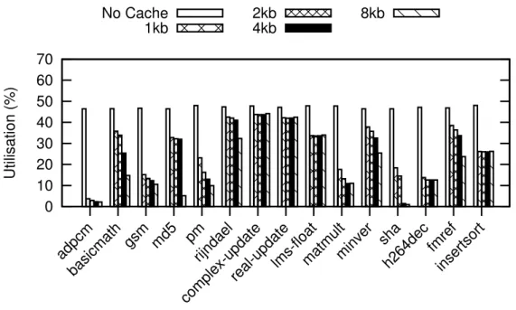
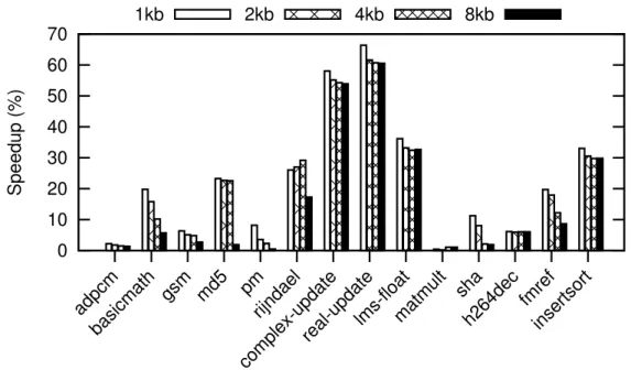
Fig. 3.3 Memory utilisation for a number of benchmarks and cache sizes. 75 Fig. 3.4 Performance increase when using basic prefetching on various benchmarks . . . 76

Fig. 3.5 Block diagram of the system model. . . 78

Fig. 3.6 Timing diagram showing the time taken for a requestω₁ to cross each functional unit in the system. . . 84

Fig. 3.7 The relationships between the inter-request times (e.g. δmem) for two requests,ω1 andω2 from the same requester. . . 84

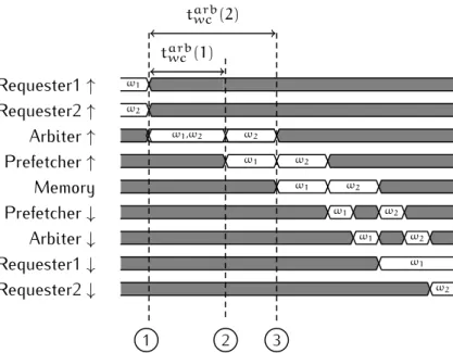
Fig. 3.8 Timing diagram showing two requests ω₁ and ω₂ dispatched from two different requesters simultaneously. . . 85

Fig. 4.1 Example Bluetree structure for an8-core system. . . 92

Fig. 4.3 Bluetree Client Packet Format. . . 93 Fig. 4.4 A timing diagram to show the blocking behaviour of a Bluetree

multiplexer for two inputs. Numbered packets (i.e. ω1) are from

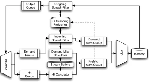
requester 1, lettered packets (i.e. ω_A) are from requester 2. This assumes a blocking factorm=3. . . 94 Fig. 4.5 Block diagram of the internals of the prefetcher. . . 102 Fig. 4.6 Timing diagram showing a single request, ω_hit, transiting the

prefetcher. This also causes a prefetch, ω_pf to be initiated. . . 105 Fig. 4.7 Timing diagram showing a single prefetch hit feedback request,

ω₁, transiting the prefetcher. This also causes a prefetch,ω_pf to be initiated. . . 105 Fig. 4.8 Timing diagram showing how a prefetch, ω_pf can be coaleasced

to a demand accessω₁ . . . 107 Fig. 4.9 Graphical view of “processor index” on Bluetree. . . 110 Fig. 4.10 Graph of execution time of a software traffic generator with and

without the prefetcher in a “worst-case” system. . . 113 Fig. 4.11 Graph of execution time of sixteen traffic generators running on

sixteen processors with the prefetcher both enabled and disabled. 114 Fig. 4.12 Change to the average-case execution time of a set of benchmarks

when the prefetcher was enabled or disabled. . . 115 Fig. 4.13 Execution times with the prefetcher enabled and disabled in the

worst-case conditions when prefetching for a single processor, and for all processors. . . 117 Fig. 4.14 Execution times with the prefetcher enabled and disabled in the

worst-case conditions, for a non-prefetchable task. . . 120 Fig. 4.15 Improvements seen by using a prefetcher on a number of

TACLe-Bench benchmarks, prefetching for only the core running the bench-mark. . . 121 Fig. 4.16 Improvements seen by using a prefetcher on a number of

TACLe-Bench benchmarks, prefetching for all cores. . . 123 Fig. 4.17 Graph of execution time of sixteen traffic generators running on

sixteen processors with the prefetcher both enabled and disabled. 124 Fig. 4.18 Change to the average-case execution time of a set of benchmarks

when the prefetcher was enabled or disabled. . . 125 Fig. 5.1 Example execution time breakdown of a hypothetical task and

architecture. . . 130 Fig. 5.2 Example execution time for a task from the memory subsystem. . 130 Fig. 5.3 Example of replacing the “missing” memory access caused by

suc-cessfully prefetching data with another memory access. In this ex-ample, access M2was successfully prefetched ahead of time and can be replaced with another prefetch, PF. . . 131

Fig. 5.4 Internals of the modified Bluetree multiplexer. . . 137 Fig. 5.5 Example of a Bluetree multiplexer relaying prefetch slots (ω_slot)

in lieu of a request. Numbered requests (i.e. ω1) are initiated

by requester 1, and lettered requests (i.e. ω_A) are initiated by requester2. This assumes a blocking counterm=3. . . 138 Fig. 5.6 Internal block diagram of the modified prefetcher. . . 141 Fig. 5.7 Timing diagram showing a standard demand read access, ω₁

transiting through the prefetcher. . . 142 Fig. 5.8 Timing diagram showing a prefetch hit request, ω_hit transiting

the prefetcher. Because there is an available candidate prefetch

ω_pf∈P₁, a prefetch can be initiated. . . 143 Fig. 5.9 Location of the small prefetch cache relative to the processor’s

own caches. . . 144 Fig. 5.10 Execution times with the prefetcher enabled and disabled in the

worst-case conditions. . . 146 Fig. 5.11 Execution times with the prefetcher enabled and disabled in the

worst-case conditions. . . 148 Fig. 5.12 Execution times with the prefetcher enabled and disabled when

an unprefetchable traffic generator is used. . . 150 Fig. 5.13 Observed execution time improvement by utilising a prefetcher

with the TACLeBench benchmarks. . . 151 Fig. 6.1 Example call graph for a hypothetical task. . . 154 Fig. 6.2 Comparison of an example data access and instruction access. . . 157 Fig. 6.3 Diagram of the internals of the intermediate stream cache. . . 158 Fig. 6.4 Example memory access scheduling with the prefetcher enabled. . 162 Fig. 6.5 Example memory access scheduling with the prefetcher enabled,

where the prefetch overlaps the demand access. . . 162 Fig. 6.6 Improvement in the WCET for a number of benchmarks when the

processor at index0was left un-connected. . . 165 Fig. 6.7 Improvement in the WCET for a number of benchmarks when the

processor at index1was left un-connected. . . 166 Fig. 6.8 Improvement in the WCET for a number of benchmarks when the

processor at index2was left un-connected. . . 167 Fig. 6.9 The performance improvement from the prefetcher being enabled

under “worst-case” conditions. . . 168 Fig. 6.10 The performance improvement from the prefetcher being enabled

L I S T O F T A B L E S

Table 2.1 Example values for t_RCD, t_CAS, t_RP and t_RAS for a variety of DDR3devices. Adapted from [11]. . . 42 Table 2.2 Area and maximum frequency for a distributed arbiter (GSMT)

versus monolithic TDM and CCSP [12]. . . 59 Table 4.1 Worst-Case blocking across a 16-core tree, measured in number

of blocks. . . 98 Table 6.1 Potential WCET savings within the analysis by using the prefetcher,

for varying numbers of cache lines in each basic block each with a given number of loads. Each cache line is assumed to be four words long. . . 164

L I S T O F L I S T I N G S

Listing 4.1 Pseudocode description of how the prefetcher handles a de-mand miss. . . 104 Listing 4.2 Pseudocode description of how the prefetcher handles a prefetch

hit. . . 106 Listing 6.1 Pseudocode description of how the stream cache inserts

incom-ing data. . . 159 Listing 6.2 Pseudocode description of how the stream cache performs a

Acknowledgements

Firstly, I’d like to thank my supervisor Neil Audsley for his help and guidance over the last four years, and for the opportunity to work on interesting projects and attend numerous conferences throughout; your help and support has been invaluable while doing my PhD. I’d also like to thank my assessors, Leandro In-drusiak, Stratis Viglas and Wim Vanderbauwhede for an enjoyable and interesting viva.

Huge thanks also go out to my friends and colleagues in CSE/120 over the past few years - Ian Gray, Gary Plumbridge, Jack Whitham, David George, Gareth Lloyd and Russell Joyce. Thanks for making a fun and welcoming, albeit at times unproductive, work environment and for your help over the course of this PhD. Thanks also to the rest of my friends in the Computer Science department and further afield throughout my time at York.

Finally, thanks go out to my family and to my partner Ione for their love and support throughout the highs, and especially the lows of the past four years - I could not have done it without you.

Declaration

I declare that all work contained within this thesis is a result of my own investiga-tions, except where explicit attribution has been given. The content of some of the chapters has already been published within the following publications:

• Jamie Garside and Neil C. Audsley: Prefetching Across a Shared Memory Tree within a Network-on-Chip Architecture. International Symposium on

System-on-Chip,2013.

• Jamie Garside and Neil C. Audsley: Investigating Shared Memory Tree Prefetch-ing within Multimedia NoC Architectures. Memory Architecture and

Organisa-tion Workshop,2013.

• Jamie Garside and Neil C. Audsley: WCET Preserving Hardware Prefetch for Many-Core Real-Time Systems. 22nd International Conference on Real-Time

Networks and Systems,2014.

This work has not previously been presented for an award at this, or any other, University.

1

I N T R O D U C T I O N

Within recent years, the breakdown of Dennard scaling [13] has limited the ability for processor designers to improve system performance by increasing the overall system clock speed. Instead, to maintain expected year-on-year performance in-creases, system designers have instead turned to scaling the number of cores on a chip rather than the core speed. Today, eight-core processor designs are becoming commonplace, and multi-core scaling is set only to continue; EZChip [14] are cur-rently creating72-core designs, Parallela are creating64-core designs which can be connected together for a maximum of 256 cores and Intel are aiming for over 60 cores on the Knight’s Landing platform [15].

While these systems are allowing apparent processor performance to meet ex-pected year-on-year improvements, they are beginning to run into an important problem. The “memory gap” has been known for the last couple of decades [16], that is, that the memory subsystem simply cannot cope with the memory band-width requirements of modern tasks. As the number of cores accessing a single memory increase, this effect is only going to worsen, and memory latencies are only going to increase.

This causes significant problems within the field of real-time systems, which by their very nature need to know the worst-case response time of all the components within a system. This rising memory latency causes the estimate for the worst-case time to execute an instruction which accesses memory to significantly increase and hence, the worst-case time to execute the task as a whole increases. As the number of cores sharing memory increases, this effect will only worsen further to potentially unacceptable levels.

There are many techniques by which some of this latency can be alleviated, one of which being prefetching. This attempts to utilise spare bandwidth to specula-tively fetch data ahead of time, although it is generally not used within real-time systems because the behaviour of the prefetcher is difficult to predict and may actu-ally cause the worst-case execution time of a task toworsen. That said, a controlled and predictable form of prefetching is an attractive prospect to try and reduce this ever-increasing memory delay by using any “spare” system bandwidth to try and reduce the execution time of other tasks.

This thesis will attempt to investigate the effects of prefetching on real-time multi-core systems, and attempt to create a prefetching scheme under which the worst-case execution time of a task can be improved. Firstly though, the remainder of this chapter will explain the background behind the move to multi-core systems

and the effects this has on real-time systems to provide the intuition behind the work in the remainder of this thesis. It will then provide a research hypothesis which this thesis will attempt to prove, before closing with a plan for the remainder of this thesis.

1.1

background

Up until the last decade, two observations managed to adequately capture the trends within computer architectures. Moore’s Law [17] states that, in effect, the number of transistors on an integrated circuit for which the cost per transistor is optimal doubles around every 18 months. Dennard Scaling [13] then states that as the feature size of transistors falls, the powerdensityof transistors remains constant and thus the power required for two identically sized dies should be the same, regardless of feature size. In effect, Moore’s Law provides extra transistors for new features, and Dennard Scaling combined with improved manufacturing processors allow the transistors to be used within a similar power budget.

While Moore’s observations are still relevant today, Dennard Scaling has begun to break down [18]. To maintain the same power density as the number of tran-sistors in a unit area increases, the power utilised per transistor naturally must decrease, for which one realisation is to reduce the operating voltage of the tran-sistor. Within recent years, this operating voltage has been lowered so far that sub-threshold leakage1

becomes a real issue and begins to limit the voltage scaling of transistors. As transistors are made smaller, the power density can no longer re-main constant and hence heat dissipation begins to become a real problem within systems.

As clock frequency increases also require more power, this led to clock frequency scaling of microprocessors to plateau around2003 [20], mainly because it is diffi-cult to dissipate the heat generated by both more transistors and faster transis-tors. This problem is then combined with increasing wire delays caused by using smaller wires [21]; as wire diameter decreases, the resistance of the wire increases and hence the time taken to switch the state of the wire between “off” and “on” increases because of the capacitor time constantτ=RC. The combination of these factors, amongst others, makes it difficult to increase the clock speed further. In-stead, to use the transistors provided by Moore’s Law and to provide the expected year-on-year performance increases, system designers instead turned to using mul-tiple cores on a single die.

1 Field Effect Transistors (FETs) used within computer circuits are effectively used as digital switches.

When there is a sufficient positive voltage between the “gate” and “source” pins of the FET (called the threshold voltage), it will allow current to flow between the “source” and the “drain” pins. Sub-threshold leakage is the current which can flow when this condition has not yet been met. This leakage is inversely proportional to the threshold voltage [19], which Dennard Scaling assumes can be lowered with transistor size in order to maintain constant power density.

CPU Memory Controller IO Controller Memory CAN CPU Memory Controller IO Controller Memory CAN

Figure 1.1:Example multi-CPU system, comprised of two independent CPUs with private memories.

While increasing the number of cores on a single chip allows for good perfor-mance increases, it does cause a new problem. Single-core processors typically contained their own memory controller, and were connected to their own memory. Any communication between processors then had to take place using a given sys-tem bus, for example, Ethernet or CAN. An example of such a syssys-tem is shown in Figure 1.1, where there are two single-core processors with exclusive access to their attached memory. If data must be shared between these processors, it must be done explicitly through the attached CAN interface.

CPU Memory Controller IO Controller CPU Memory CAN

Figure 1.2:Example multi-core system, comprised of a dual-core CPU with a single shared memory.

Due to many factors, allowing each core to retain its own private, software man-aged memory is infeasible in multi-core processors. Constraints such as die area, power utilisation and the number of package pins [16] limit the number of memory modules that can be connected to a chip and hence make it impossible for each processing core to have its own large, private memory. Instead, each core must

share the global system resources, creating a system such as that shown in Fig-ure1.2. Within this system, both cores share a single common memory controller and I/O controller. For the aforementioned reasons, these controllers are rarely multi-channel and hence if both cores want to access memory at the same time, there will be contention and one of the cores will be granted access to memory, causing the other to have to wait.

This contention causes significant issues within the field of real-time systems. A real-time task is typically characterised by the fact that it must respond to an input stimulus with a set period of time for the output to be valid. There are various examples of such systems; flight control systems must process the pilot’s inputs quickly and update the state of the aircraft’s control surfaces quickly enough to be responsive, video decoders must emit a new frame with a set deadline to ensure smooth video playback. To make such guarantees, a real-time task can be evalu-ated against a model of the system to ascertain a worst-case execution time for a portion of the task’s code. Given that the execution time of a block of code can be bounded, it is then possible to assert that a task can respond to a given input in a given period of time.

To construct this system model, it must be possible to determine how long each component in the system will take to respond in the worst-case. For a task which uses external memory, it must therefore be possible to ascertain the worst-case time to access memory in order to create a worst-case bound on the task as a whole. For a system using single-core processors such as that in Figure 1.1, the worst-case response time of the memory is simply the worst-case time for the memory controller to operate. In a multi-core system such as that in Figure 1.2 with a shared memory controller, however, the problem is much more complex. Not only does the response time of the memory controller need to be known, but it must also be possible to ascertain what the other processors are doing at that point in time to determine if any of their memory accesses will block any given memory access.

Analysing how these tasks will interfere is possible [22,23], but difficult; if the tasks running on each processor can be started and stopped at will, the blocking caused between each set of tasks which may execute together must be considered, a problem which is exponential in nature [24] and hence soon becomes infeasible as the number of tasks grows.

A method by which this complexity can be alleviated is to assign each task a partition of the available system bandwidth which describes the portion of the system bandwidth which can be given to a task, and the maximum latency between issuing a request and the request being given service. These constraints are then enforced using a hardware arbiter sitting between the processors and memory, which ensures that no processor can cause any other processor to receive less than its defined bandwidth. A revised version of the system design with an arbiter is

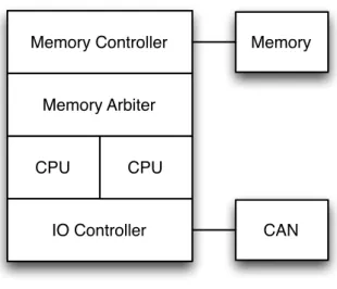
CPU Memory Controller IO Controller CPU Memory CAN Memory Arbiter

Figure 1.3:Example multi-core system, comprised of a dual-core CPU with a single arbi-trated shared memory.

shown in Figure1.3. By splitting the system bandwidth like this, the system model can use the given constraints of the assigned partition when determining the worst-case response time for a memory access. Because the bandwidth partitioning is enforced by the arbiter, the interference caused by other processors need not be considered when analysing the execution time of a task, since the arbiter will ensure that the task receives the level of service defined by the partition.

While this approach makes the worst-case analysis of the system simpler, and can provide additional safety guarantees, it does have its problems. This approach effectively places a static bound on the amount of blocking that any memory re-quest can experience, and thus assumes that all other processors are fully utilising their bandwidth bound (or even that all available system bandwidth has been allo-cated). If this is not the case, then there will be “spare” system bandwidth available. Moreover, because the estimate for the worst-case response time of a memory ac-cess assumes a request will be blocked by many other proac-cessors issuing memory accesses, the worst-case response time of a memory access increases as the number of processors increases.

This problem is being further exaggerated by another issue. While processors have seen bountiful year-on-year performance increases, seeing year-on-year per-formance increases of 1.25x to1.52x, the memory side of things has not been so lucky. Memory performance scaling has only been growing year-on-year at a rate of around 1.07x [1], leading to the so called “memory gap” as seen in Figure 1.4. As processor speeds increase and the degree of memory sharing increases, as will the apparent cost of accessing memory.

There has been some improvements in memory technology to alleviate this per-formance gap; modern DDR memories contain multiple “banks” of memory which can be accessed in parallel to attempt to alleviate contention issues when sharing

5.1 Introduction

289

block

(or

line

), are moved for efficiency reasons. Each cache block includes a

tag

to see which memory address it corresponds to.

A key design decision is where blocks (or lines) can be placed in a cache. The

most popular scheme is

set associative

, where a

set

is a group of blocks in the

cache. A block is first mapped onto a set, and then the block can be placed

any-where within that set. Finding a block consists of first mapping the block address

to the set, and then searching the set—usually in parallel—to find the block. The

set is chosen by the address of the data:

(Block address)

(Number of sets in cache)

If there are

n

blocks in a set, the cache placement is called

n-way set associative

.

The end points of set associativity have their own names. A

direct-mapped

cache

has just one block per set (so a block is always placed in the same location), and a

fully associative

cache has just one set (so a block can be placed anywhere).

Caching data that is only read is easy, since the copy in the cache and

mem-ory will be identical. Caching writes is more difficult: how can the copy in the

cache and memory be kept consistent? There are two main strategies. A

write-through

cache updates the item in the cache

and

writes through to update main

memory. A

write-back

cache only updates the copy in the cache. When the block

is about to be replaced, it is copied back to memory. Both write strategies can use

a

write buffer

to allow the cache to proceed as soon as the data is placed in the

buffer rather than wait the full latency to write the data into memory.

Figure 5.2 Starting with 1980 performance as a baseline, the gap in performance between memory and processors is plotted over time. Note that the vertical axis must be on a logarithmic scale to record the size of the processor-DRAM performance gap. The memory baseline is 64 KB DRAM in 1980, with a 1.07 per year performance improvement in latency (see Figure 5.13 on page 313). The processor line assumes a 1.25 improvement per year until 1986, and a 1.52 improvement until 2004, and a 1.20 improvement thereafter; see Figure 1.1 in Chapter 1.

1 100 10 1,000 P erf or mance 10,000 100,000 1980 1995 2000 2005 2010 Year Processor Memory 1990 1985

Figure 1.4:The growing gap between CPU and memory performance [1]

a single DDR memory. As an example, Micron’s1Gb DDR3modules are arranged as eight banks [11], with newer DDR4memories containing up to sixteen banks of memory [25]. Of course though, each bank can only be accessed by one requester at once, hence the system designer must ensure that all banks are being utilised in a uniform manner by all requesters to ensure optimal system performance. While this reduces the interference which a task may experience when accessing memory, there is still the very real problem of contention within the banks, and the actual rising latency of a single memory request to deal with.

Of course, this rising memory latency has spawned much work to attempt to mask these latencies. One of these methods is caching [26], which attempts to store recently used data close to the processor to attempt to drastically reduce the latency of accessing frequently used data. Examples of where this is useful are loops, where the same code will be executed many times, or for a few data items which are frequently accessed (e.g. counters or state variables). While this technique can mask the latency of frequently accessed items, it does nothing to attempt to mask the latency of the “initial” load of a data item. Caching therefore does not have much of a positive effect on a task which accesses each member of a data set only once, or has very large, straight blocks of code since every memory access will cause a cache miss (i.e. the required data will never be resident in cache).

As mentioned earlier, systems which use partitioned bandwidth may not fully utilise the available bandwidth, leading to some “spare” bandwidth within the system. Another method to alleviate the rising worst-case cost that can also use some of this spare bandwidth is prefetching. A prefetcher is a functional unit within the system which attempts to predict what a requester will soon require,

and issue a memory request on behalf of that requester ahead of time. As an example, if a requester accesses addresses A,A+1andA+2in sequence, it will probably require the data at address A+3 in the near future. This is a rather naïve metric; other, smarter metrics are explored further within Section 2.4. If the prefetcher was accurate, it will reduce the latency of a memory access vastly, because the required data will already have been delivered to the processor ahead of time. This method can also be combined with caching; caching can reduce the latency of repeatedly accessed data, and prefetching can attempt to fetch the “next” data into cache ahead of time to reduce the cost when data has not been previously accessed.

Ultimately, however, both techniques cause issues when used within real-time systems as they modify thecontextunder which a task is being executed. In order to determine the latency of a memory access when a cache is used, the system model must also consider all other memory accesses which have previously taken place to determine whether the required data is resident in cache. While this is simple for single path tasks, it is generally undecidable if a task’s control flow de-pends on its input data [27]. As the memory access pattern then depends upon the path taken through the program, a static analysis tool cannot accurately de-termine what data has been fetched and hence what is stored in cache unless the input data is known a priori. This leads to an estimate for the worst-case execution time which is lowerdue to the inclusion of the cache, but pessimistic because the behaviour of the cache cannot be predicted with perfect accuracy.

Prefetching also suffers from a similar problem: the state of the prefetcher is context sensitive depending on what accesses the prefetcher has observed where again, the run-time behaviour of a task based upon its inputs will change the be-haviour of the prefetcher. Moreover, the accesses which the prefetcher observes are based upon the behaviour of the cache. If the system analysis cannot deter-mine for definite whether a requested data item is resident in cache, then it cannot also determine whether the prefetcher observes said data access and hence cannot make any guarantees about the state of the prefetcher. Because the cache analy-sis is undecidable, the prefetcher’s state is hence undecidable and thus the set of memory accesses issued by the prefetcher are undecidable. On top of this, many prefetchers fetch directly into the processor’s cache rather than any form of hold-ing buffer, hence caushold-ing further unpredictability regardhold-ing the contents of the processor’s cache; the prefetcher may have fetched useful data, but could well also have displaced useful data already resident in cache, hence invalidating much of the existing cache analysis.

Despite these problems, something needs to be done to slow down the rising memory latencies in real-time systems. This work explores using prefetching within the context of a real-time system to attempt to improve the time which an executing task is blocked waiting for memory accesses to complete. This

chap-ter will first further explore the reasons for moving to shared-memory multi-core systems, before using this information to form a research hypothesis for the re-mainder of this thesis and finally providing a structure for the rere-mainder of this thesis.

1.2

research hypothesis

As introduced in Section 1.1, caching is a good way to hide some of this memory latency. The problem is, caching does not actually reduce memory latency, only hides the latency involved with fetching repeated data, which it does by moving recently accessed data closer to the processor into faster storage. Caches also typ-ically fetch data on the granularity of an entire cache line (of the order of 16-32 bytes of data), hence also hide the latency of accessing some subsequent mem-ory locations to the one originally accessed. While this optimises the number of memory accesses that take place though, it does not actually optimise how these memory accesses take place; even if some memory accesses no longer take place, those that do will still incur large latency costs.

It is clear that if memory delays are to increase along this trajectory for the foreseeable future, the memory system must be optimised as a whole. Moreover, something needs to be done about the growing pessimism within real-time sys-tem analysis brought about by the memory subsyssys-tem. Prefetching is an attractive optimisation to use for this; by pushing data out from memory to the processors speculatively, the costs involved with memory access can be reduced, or even re-moved entirely.

Of course though, this causes problems for real-time systems. A prefetch unit within the system speculatively requesting data from memory can cause extra interference for running tasks, and since prefetchers normally deliver data directly into the cache of the target processor, it may also invalidate any cache analysis. For the most part however, these limitations are simply because prefetching, as of yet, has not been considered under the constraints of a real-time system. If the prefetcher can be constrained in a way such that it is possible to predictwhatit will do andwhen, there is no real reason why it cannot be used in a real-time system.

This thesis will therefore explore the following hypothesis:

A prefetcher can be constructed so that it can be used within a real-time system in a predictable way, such that it does not cause any detriment to the worst-case execution time of the tasks running within that sys-tem. Furthermore, it is possible under certain circumstances to predict when the prefetcher will operate, allowing it to utilise “spare” or unallo-cated bandwidth within the system to actively improve the worst-case execution time estimate of a task running in a real-time system.

1.3

thesis structure

From this, the remainder of the thesis will be structured as follows:

chapter 2 will detail the related literature in the subjects of multi-core systems,

including how to predict the behaviour of DRAM, how to arbitrate multiple requesters fairly for DRAM, and current work related to prefetching on both single and multi-core systems.

chapter 3 will, given the related literature, further concrete the chosen research

avenue and provide a research hypothesis

chapter 4 demonstrates the effects brought about by using a traditional,

non-arbitrated prefetcher and the potential system analysis issues it brings about. chapter 5 will provide a framework by which a prefetcher can be integrated

into a real-time system without affecting the worst-case execution time of the system.

chapter 6 will then provide a method by which a prefetcher can be used in order

to improve the calculated worst-case execution time.

chapter 7 will then, finally, provide the major conclusions identified and outline

2

B A C K G R O U N D & R E L A T E D W O R K

This chapter will provide a concise overview of the related literature within the fields of work associated with real-time prefetching. This will first give an overview on the operation of memory within systems, the problems it poses within a real-time system, and how these issues are handled within the current state of the art. It will then provide an overview of current caching and prefetching schemes, before detailing how shared resources are arbitrated in both monolithic and dis-tributed fashions. It will then give a brief overview of scheduling theory and how predictability is asserted, before summing up by outlining the methods by which a program can be analysed and a worst-case bound ascertained.

2.1

predictability

There are many variations on the definition of a real-time system. The common definition is effectively that “a system which must, by a defined time period, be able to react to an external stimulus from the environment”. An external stim-ulus may be anything from a user pressing a button on the system to a video transcoder receiving video to a nuclear reactor reaching the point of no return before meltdown.

Of course, each of these scenarios are vastly different in terms of scale. A user will only be slightly inconvenienced if a system takes a while to respond to the play button being pushed. If a video encoder fails, there might be some frame skip. If a reactor goes critical or an aircraft fails to respond to input, it could lead to loss of life. For this reason, the real-time community tends to split up the definition of real time between hard real-time, firm real-time and soft real-time (HRT, FRT and SRT, respectively). These are defined by Burns and Wellings [28] as follows: hard real-time Where it is absolutely imperative that the system reacts within

its given time frame, else there may be disastrous consequences.

firm real-time Where the deadline may be missed occasionally, but there is no benefit from it being late.

soft real-time Where the deadline may be missed occasionally, or that a service can occasionally be delivered late.

In the case of both FRT and SRT tasks, there may be an upper limit on the num-ber of times there can be a deadline miss. To quote the video encoder example again, a couple of late frames is nottoo bad; it just leads to a slightly poor expe-rience. Many late frames within a short interval, on the other hand, renders the video almost unwatchable. Additionally, as stated also by Burns and Wellings, a system may have both HRT and SRT requirements, for example, a warning system may have a SRT deadline of50ms for optimal response, while a HRT deadline of 200ms also exists to prevent damage.

For this task, it is vital to determine the range of times in which a task may execute for in order to prove that a task may meet these constraints. As noted by Wilhelm et al. in their review of worst-case execution time prediction methods [2], this is generally done by observing the execution of a task under a variety of test cases and recording the monitored best and worst case execution times. Of course, this will overstate the best case and understate the worst case, as an exhaustive analysis can be difficult to perform and as such, is not applicable for HRT tasks. Standard techniques in industry for predicting the real worst case execution time (WCET) may place constraints on the activities that can be performed within a program (e.g. forbidding recursion).

Of course, there are a vast number of ways to arrive at a WCET estimate or bound, and the remainder of this section shall attempt to provide an overview of the techniques which can be used. Again, this is to attempt to bring the reader up to speed with the terminology and techniques used, nor explain each method in great depth and does not attempt to be an exhaustive search through the liter-ature surrounding time predictability, which would be another review in itself. If desired, there are many reviews in existence, such as the2000review by Puschner and Burns [29] and a review from2008by Wilhelm et al. [2].

2.1.1 Deriving Predictability Estimates and Bounds

There are two main classes of approaches used to derive a predictability bound and/or estimate. In this context, a boundcannotbe exceeded, else the analysis is wrong. An estimate, on the other hand, is not100% guaranteed to be correct, but should be accompanied with an error margin.

Static Analysis

Static analysis is typically an offline technqiue which attempts to ascertain a worst-case bound of a given section of a task by using a model of the target architec-ture [30]. This is performed in a number of steps [31]:

flow analysis, using the source and the final output, reconstructs all the possi-ble paths through a program. For this, certain constructs, e.g. recursion, may not be permitted due to their ambiguity in analysis, or may have to be manu-ally constrainted by the programmer to assert facts about them, for example, maximum loop iterations or recursion depth.

global low-level analysis computes the factors affecting a task on a certain machine from the machine’s global constructs, for example, cache.

local low-level analysis computes the same factors as above, but localised to a single task and code segment, for example, pipeline stalls and branch prediction.

The end result is then calculated from these three components. There may also be other inputs in order to make the task easier, for example, value analysis, as detailed by Ferdinand et al. [32] approximates the state that each processor register can be in at run time. This can then be used to compute the range of possible memory addresses that can occur at run time and thus aid in cache analysis.

Of course though, in order for this technique to be sound, it requires an ex-tremely accurate model of the processor. This is simple for a basic architecture (for example, Z80); each instruction takes a fixed number of cycles and all memory accesses are single-cycle. Of course, modern architectures are much more com-plex than this. For example, in order to ascertain what the effect of a cache on the worst-case execution time is, the analysis must attempt ascertain what the con-tents of cache will be at any point in time. Persistence analysis is typically used for this [33], which for each memory access classifies if it is definitely not in cache (e.g. for the cases where analysis cannot definitely ascertain that the same cache line has already been loaded and not evicted), or those whichmayreside in cache (e.g. an earlier access in the flow analysis accessed the same line).

As will be explored further in Section2.2, the unpredictability of memory also adds difficulty to the static analysis of a given task. The access time to a given location in memory depends upon the previous pattern of accesses; if an access is accessing the same DRAM line as the previous access, the memory access will be much faster than for a different row. Moreover, as multi-core systems become more prevalent, static analysis must ascertain how long an access to a shared memory resource takes given the interference from other tasks in the system. Techniques to derive this will be explored further in Section2.3.

These factors lead to problems with pessimism in static analysis. As it is diffi-cult to soundly assert conditions on the state of the system, many static analysis techniques must assert case conditions on each access. As an example, worst-case memory access latencies are normally assumed and worst-worst-case initial cache conditions must be assumed. Moreover, in order to make the problem feasible to solve, many analysis tools will limit the number of blocks that the state of caches is

asserted over, and hence may assume that cache blocks are missing when they will definitely reside in cache. Despite this pessimism, static analysis should always be able to find the worst-case path, assuming that the model of the processor is sound and is hence typically regarded as safer than measurement-based approaches.

Measurement-based Analysis

Rather on relying upon an accurate model of the processor, measurement-based analysis instead uses the behaviour of the processor itself to model the execution times [34], after all, “the best model of the processor is the processor itself”. As with static analysis, measurement based techniques begin by re-constructing a flow graph of the program, where each block in the graph typically corresponds to a single-entry single-exit block of instructions which are executed sequentially, typ-ically known as a basic block. The tool then executes the program a number of times under a set of inputs and environmental conditions, then times how long each of these blocks takes to execute to derive a distribution of probabilities for each block.

After this has taken place for each block, the execution times for each block can be combined according to the flow graph. If blocks are connected in a sequential fashion, then the execution times of each are summed, if they appear in parallel (e.g. in an if/then/else construct), then the maximum execution time of all of the parallel blocks is selected. The combination of all of these basic blocks then forms an estimate of the worst-case execution time of the entire task.The Worst-Case Execution-Time Problem • 36:3

Fig. 1. Basic notions concerning timing analysis of systems. The lower curve represents a subset

of measured executions. Its minimum and maximum are theminimalandmaximal observed

exe-cution times, respectively. The darker curve, an envelope of the former, represents the times of all

executions. Its minimum and maximum are thebest-andworst-case execution times, respectively,

abbreviated BCET and WCET.

exhaustively explore all possible executions and thereby determine the exact worst- and best-case execution times.

Today, in most parts of industry, the common method to estimate execution-time bounds is to measure theend-to-endexecution time of the task for a subset of the possible executions—test cases. This determines the minimal observed andmaximal observed execution times. These will, in general, overestimate the BCET and underestimate the WCET and so are not safe for hard real-time systems. This method is often calleddynamic timing analysis.

Newer measurement-based approaches make more detailed measurements of the execution time of different parts of the task and combine them to give better estimates of the BCET and WCET for the whole task. Still, these methods are rarely guaranteed to give bounds on the execution time.

Bounds on the execution time of a task can be computed only by methods that consider all possible execution times, that is, all possible executions of the task. These methods use abstraction of the task to make timing analysis of the task feasible. Abstraction loses information, so the computed WCET bound usually overestimates the exact WCET and vice versa for the BCET. The WCET bound represents the worst-case guarantee the method or tool can give. How much is lost depends both on the methods used for timing analysis and on overall system properties, such as the hardware architecture and characteristics of the software. These system properties can be subsumed under the notion oftiming predictability.

The two main criteria for evaluating a method or tool for timing analysis are thussafety—does it produce bounds or estimates?— andprecision—are the bounds or estimates close to the exact values?

Performance prediction is also required for application domains that do not have hard real-time characteristics. There, systems may have deadlines, but

Figure 2.1:Graphical view of the execuiton times of a task, along with the relevant bounds [2].

In order to be sound, this approach must be able to assert that it has actually observed the worst-case path through the task and the worst-case conditions of the system. An example of this is shown in Figure2.1, where the meaning of each item is explained as follows:

measured execution times: Observed maximum/minimum execution times for the task. These may not be accurate, as the actual maximum/minimum exe-cution times may not have been observed.

bcet/wcet: Actual best and worst-case execution times. These may occur very infrequently and hence were never observed.

upper/lower timing bound: Best and worst case execution times with a safety margin added.

measured execution times: The set of all execution times observed when eval-uating the worst-case behaviour of the task.

possible execution times: The set of all possible execution times for all differ-ent program paths, inputs and initial hardware conditions.

timing predictability: The possible range of execution times after the safety margin has been added.

In this example, the actual highest execution time may have been observed as “maximal observed execution time”, but the actual worst-case under a different set of conditions may be much higher at the “WCET” line. The first solution is the observe the flow graph in order to assert that full program coverage has been achieved. If this cannot be asserted, then it is possible that a block of code has been missed with an extremely high actual execution time. The second solution is to exhaustively test all possible inputs, and execute the code with a sufficient number of iterations such that all possible system states haveprobablytaken place. While simpler than static analysis techniques, it is much more difficult to assert that a measurement-based analysis is sound because of the unpredictability of sys-tem compontents such as caches and shared memory. While dynamic anaysis does work on multi-core system, it does have to be constrained such that the memory arbiter is also operating in worst-case conditions in order for the actual worst-case execution time to be observed, which may again be difficult without modifying the arbiter itself.

2.1.2 Response Time

The predictability of a system is also not only dependant upon the worst case execution time of a single task. In general, the WCET of a task assumes a sole task running with no interference. Clearly, on a system, interrupts can arrive, a process can be pre-empted to make way for a higher priority task, or a required resource may not be available as another task it currently using it. For this reason, the deadline of a task is normally much longer than the actual WCET of a task. In general, the worst case response time Rof a taskiis denoted as R_i=B_i+C_i+I_i

as outlined by Burns and Wellings [28]. C_iis the WCET of process iandI_i is the interference processireceives, be it pre-emption, locked resources, or anything else influenced by other processes within the system. Bi is the blocking factor which

the maximum time spent on acquiring shared resources and critical sections. This analysis goes on to detail the blocking factor I as follows, given fixed priority scheduling:

InterferenceI_i

Given all tasks in the system with a higher priority,hp(i), the maximum amount of interference is as follows, given thatT_iis the period of taski.

I_i= X j∈hp(i) R_i T_j C_j

This equation can be extended to include the time taken to perform a context switch [28], the time to overcome a polluted cache from the pre-empting pro-cess [35], and generally the time to recover the state of the system at the time the process was pre-empted. An example extension to this is as follows:

I_i= X j∈hp(i) R_i T_j (CS1+CS2+C_j+γ_j)

Where CS1 and CS2 are the times taken by the operating system to context switch away from and back to a task, respectively. γ_jis then the delay imposed on taskiby the cache pollution introduced by taskj.

BlockingBi

The blocking factor B is a much simpler factor to compute. Assuming a priority inheritance protocol [36], where a task utilising a shared resource assumes the priority of the highest consumer of that resource when using it, the blocking factor is the sum of the time taken in all critical sections where said critical section is used by a process with lower priority than process i, and also by a process with equal or higher priority toi.

This blocking term exists solely because it is possible for a lower priority task to lock a resource used by a higher priority task (as the normal execution time with the lock is accounted for byI_i. Since priority inheritance ensures that each critical section can only be blocked by a lower priority task once for each critical section, for the duration of that critical section [36]. Hence, given K critical sections, that

task priority i(and0otherwise), and thatC(k)is the WCET of the critical section k: Bi= K X k=1 usage(k,i)C(k)

2.1.3 Priority Ceiling Protocol

The model detailed previously assumes a priority inheritance protocol is used, where a user of resource assumes the priority of the job it blocks with the highest priority. This is to prevent “priority inversion” from occurring, where a low prior-ity taskaobtains a shared resource, then is preempted. If a higher priority taskb

attempts to use the shared resourcewithouta priority inheritance protocol, it will be blocked until taskahas finished with the resource. If there are also other tasks with their priorities in between tasksaandb, taskawill still have to wait for those tasks to complete (or block), and as such, have to wait much longer to execute its critical section, thus further blocking taskb.

Another protocol is the Priority Ceiling Protocol, also suggested by Sha et al [36]. This was designed to address some of the flaws in priority inheritance, for example, that it is possible for transitive blocking to occur (high priority taskcblocked byb

blocked by low priority taska), and that deadlock is possible (e.g. a high priority task c wanting to lock a resource owned by a, which in turn wants to lock a resource owned by c). This takes two forms: the original ceiling priority protocol and the simpler immediate ceiling priority protocol.

From Burns and Wellings [28], the original priority ceiling protocol takes the following form.

1. Each task has a static default priority

2. Each resource has a static ceiling value defined, which is the maximum pri-ority of the tasks which use it.

3. Each task has a dynamic priority, which is the higher of its own priority, and any inherited from blocking higher priority tasks (same as priority inheri-tance).

4. A task can only lock a resource if its dynamic priority is higher than the ceiling of any locked resource (unless those resources belong to that task). Clause 4 prevents some of the properties listed above. Taking the deadlock example, when the higher priority task attempts to lock something which the lower priority task would require, since its dynamic priority is not strictly greater than

the current system ceiling. It would then not be allowed to access the resource and would be blocked by the lower priority task until said lower priority task had finished with the shared resource, and the system ceiling was again lowered.

The immediate ceiling priority protocol is similar, but much easier to implement. In this case, when a task acquires a shared resource, its priority is raised to the priority ceiling of the shared resource (that is, immediately assumes the priority of the highest priority task which could utilise the resource).

Within both priority ceiling protocols, the blocking factorB_iis changed to [28]:

B_i=maxK

k=1 usage(k,i)C(k)

This is, simply enough, the length of the longest critical section in any lower priority task which is shared with the current task. This holds because when a low priority task obtains a lock on a resource which could be used by a high priority task, no other tasks may lock any resource which can be used by the high priority task. Given that, a high priority task may be blocked by a single lower priority task. Assuming nested locks, a task may be blocked multiple times, but it may only be blocked by a single task.

2.2

memory

Of course, in order for a processor to be able to perform any useful computation, it needs access to some form of memory. Traditionally, this would have been some form of static-RAM (SRAM) device, and is effectively implemented as a flip-flop connected to two transistors to control access to the cell. In a typical implemen-tation, this utilises approxamately six transistors, as can be seen in Figure2.2. In order to access SRAM, W line of the word to read is asserted by an address de-coder based upon the input address, then the data stored in the flip-flop is sensed through theBlines.

This design leads to a chip which consumes reasonably little power and is fast. More importantly, however, is the fact that it is predictable; since the device is effectively a set of flip-flops connected to a multiplexer, the access time is related to the propogation delay of the internal logic, and both reads and writes typically take the same amount of time to complete.

While SRAM performs well and is simple to predict, the design of each cell makes it infeasible to use for large-scale shared memories typically required on modern systems. The number of components in each cell makes each cell large in silicon, hence it suffers from poor density and as a result it is expensive to create large SRAM chips. In a world dictated by cost, this makes DRAM an attractive

Word Line

Bit Line

Transistor Capacitor Plate

Source: ICE, "Memory 1997" 19941

+V W B B To Sense Amps 18471A Source: ICE , "Memory 1997"

SRAM DRAM

Figure 2.2:Comparison of SRAM and DRAM designs, adapted from [3] .

alternative. Each DRAM cell is implemented using a capacitor connected to a single access transistor, as can be seen in the first half of Figure 2.2, giving each DRAM cell a much smaller footprint than the SRAM equivalent and hence allow-ing devices to have much higher storage densities. This makes DRAM attractive to any situation where large amounts of storage are required (e.g. external memory), leaving SRAM to be used for smaller amounts of faster storage, such as processor caches and scratchpads.

These density gains are not without any cost, however; DRAM has many flaws stemming from the usage of capacitors as a storage medium [5]. The first of these is that capacitors leak charge over time. In order to mitigate this issue, the DRAM controller must periodically refresh the contents of these capacitors in order to maintain the charge stored within and prevent bit flips from occuring. This takes a period of time within which the memory cannot accept any other memory requests, as the refresh cycle effectively reads an entire DRAM row out and writes it back again. As an example, a modern 1Gb Micron DDR4 module requires a refresh which takes 260ns every 7.8µs [25]. This both slows down the potential access time, and makes DRAM less predictable; the total access time now depends on whether a refresh cycle needs to take place first.

As RAM sizes increase, it is not practical to simply carry on adding more and more rows to the RAM chip; the resulting die would be extremely long and very narrow. To alleviate this, denser SRAM and DRAM cells add more DRAM rows, but also make each row longer; as an example, a single 256Mb DDR3 module has a row size of 2Kb [11]. Due to physical and electrical constraints, it is clearly impossible to transmit all2048of these bits from the package at once (to contrast,

Chapter 7 OVERVIEW OF DRAMS 321

the bitline voltages all the way to logic level 0 or 1. Bringing the voltage on the bitlines to fully high or fully low, as opposed to the precharged state between high and low, actually recharges the capacitors as long as the transistors remain on.

Returning to the steps in handling the read request. The memory controller must decompose the pro-vided data address into components that identify the appropriate rank within the memory system, the bank within that rank, and the row and column inside the identifi ed bank. The components identifying the row and column are called the row address and the col-umn address. The bank identifi er is typically one or more address bits. The rank number ends up causing a chip-select signal to be sent out over a single one of the separate chip-select lines.

Once the rank, bank, and row are identifi ed, the bitlines in the appropriate bank must be precharged

(set to a logic level halfway between 0 and 1). Once the appropriate bank has been precharged, the sec-ond step is to activate the appropriate row inside the identifi ed rank and bank by setting the chip-select signal to activate the set of DRAMs comprising the

desired bank, sending the row address and bank identifi er over the address bus, and signaling the DRAM’s ____RAS pin (row-address strobe—the bar indi-cates that the signal is active when it is low). This tells the DRAM to send an entire row of data (thousands of bits) into the DRAM’s sense amplifi ers (circuits that detect and amplify the tiny logic signals repre-sented by the electric charges in the row’s storage cells). This typically takes a few tens of nanoseconds, and the step may have already been done (the row or page could already be open or activated, meaning that the sense amps might already have valid data in them).

Once the sense amps have recovered the values, and the bitlines are pulled to the appropriate logic levels, the memory controller performs the last step, which is to read the column (column being the name given to the data subset of the row that is desired), by setting the chip-select signal to activate the set of DRAMs comprising the desired bank,2 sending the column address and bank identifi er over the address bus, and signaling the DRAM’s ____CAS pin ( column-address strobe—like ____RAS , the bar indicates that it is

DRAM Bank

Column MUX Sense Amps

Row

Decoder One DRAM Page

One Column

ROW ADDRESS

COL ADDRESS

FIGURE 7.8: The multi-phase DRAM-access protocol. The row access drives a DRAM page onto the bitlines to be sensed by the sense amps. The column address drives a subset of the DRAM page onto the bus (e.g., 4 bits).

2_{This step is necessary for SDRAMs; it is not performed for older, asynchronous DRAMs (it is subsumed by the earlier} chip-select accompanying the RAS).

Figure 2.3:Internal organisation of DRAM cells, from [4] .

the package has only78pins). Instead, a column decoder is also employed in order to select which bits within a row are required, and the RAM is addressed using a row/column scheme where part of the requested address form the row to read from, and the remainder select the respective column.

While SRAM cells can typically be addressed directly using this matrix scheme, DRAM is more difficult. Firstly, each bit is stored using a small capacitor (of the order of 20-30 fF [37]), hence there is not enough charge stored within to drive standard logic pins. Instead, when a row is selected, the cells in the addressed row drive a set of sense amplifiers, which detect the small amounts of charge (or lack thereof) and drive a logic ‘0’ or ‘1’. Due to the capacitor time constantT =RC, this takes time, and hence there is a required time interval between selecting the row and being able to select the column. Due to this restriction, and to reduce device pin counts, the row and column are typically selected as two separate commands, denoted as “RAS” and “CAS”.

There is also additional time as reading a DRAM cell is a destructive operation, since charge is drained from the capacitors to drive the sense amplifiers. Because of this, the sense amplifiers must write the data read back into the DRAM cells again in order to prevent data loss. After data has been read or written, the sense amplifiers must be reset to a known state again. This is done by driving them to a voltage level in-between logic ‘0’ and ‘1’ such that the small amount of charge stored in the capacitor (or lack thereof) will drive the charge stored in the sense amplifier towards the respective logic level through a process called “precharging”. Both the writing back of read data and precharging of course, takes additional latency.

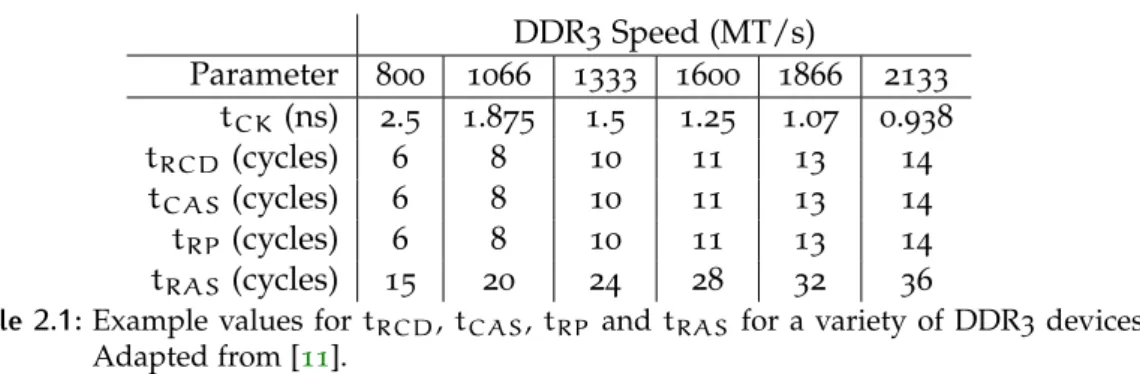
The net result of this is that there is a set of latencies that need to be adhered to in order to be able to utilise a DRAM module, as follows:

tRCD: RAS-to-CAS latency. The time between issuing a row selection (RAS) and column selection (CAS)

t_CAS: CAS latency. The time between issuing a column selection and the selected data being available.

t_RP: Precharge delay. The time between a precharge being issued and being able to select a new row.

t_RAS: Active to precharge delay. The minimum time between opening a page (by issuing RAS) and closing it again (by issuing a precharge).

tRCD tCAS tRP tRAS 1 2 3 4 5 CLK WE CAS

Addr Row Col Row

DQ D D

Figure 2.4:Example timing diagram for a DRAM read cycle, adapted from [5]. It is

as-sumed that all commands are latched on the rising clock edge.

The relationships between these timing constraints can be found in Figure 2.4, where the major stages are described as follows:

1. A row address is placed on the DRAM’s address lines, and RAS is asserted to signal the DRAM to latch the address.

2. Aftert_RCD cycles, the controller must now place the column address on the DRAM address lines and assert CAS to latch the address.

3. The DRAM module makes the requested data available after another t_CAS cycles. In this case, the module outputs two words of data to the controller. 4. After a minimum of t_RAS cycles after the first RAS has been issued, the

controller can choose to issue a precharge command if it wishes to access another row, typically done by asserting both RAS and WE simultaneously. This command can overlap with the data output stage as shown, as long as thet_RP constraint holds.

5. t_RP cycles after issuing the precharge command, the memory module can then accept the next row address, and the process starts afresh.

These specified latencies typically depend upon both the target data rate of the device, and the speed grade of the individual part in use and are typically ex-pressed as a number of clock cycles. Example figures for these latencies, along with the associated clock frequency can be found in Table2.1.

DDR3Speed (MT/s) Parameter 800 1066 1333 1600 1866 2133 t_CK (ns) 2.5 1.875 1.5 1.25 1.07 0.938 tRCD (cycles) 6 8 10 11 13 14 tCAS(cycles) 6 8 10 11 13 14 t_RP (cycles) 6 8 10 11 13 14 t_RAS (cycles) 15 20 24 28 32 36

Table 2.1:Example values fortRCD,tCAS, tRP andtRAS for a variety of DDR3devices.

Adapted from [11].

Because of the latency required between selecting a row and being able to select a column, and the time taken to precharge the row again, many memory controllers attempt to keep the currently selected row open in the hope that the next access will hit the same row [4]. While this tends to yield good performance benefits for tasks which access sequential data, it further harms the predictability of DRAM; the timing of an access now also depends upon the addresses of the accesses which came before it. Moreover, a period of time must be waited after switching from a read to a write, or vice versa, due to the time it takes to reverse the direction of the data bus, further harming predictability.

The net result of these issues is that DRAM is difficult to predict compared with the simpler SRAM design since the latency of an access depends upon the previous accesses and whether the memory controller scheduled a refresh cycle at that point in time. Of course, it is possible to assume the worst-case timing on every single access (i.e. each access causes read/write switching and a precharge to take place), but this causes the efficiency of the memory subsystem to suffer (to around 40% efficiency on DDR2 devices [38] and falling further for DDR3 devices). This is, of course, unacceptable for modern systems. Much work has gone into improving the predictability of DDR systems while attempting to retain some of the efficiency, which will be explored throughout the remainder of this section.

2.2.1 Predictable DRAM Access AMC

Paolieri et al. present a new memory controller called AMC (Analysable Memory Controller) [39]. It is designed such that each task can be independently analysed;