Game Theoretic Model Predictive Control for Autonomous Driving

GAME THEORETIC MODEL PREDICTIVE CONTROL FOR AUTONOMOUS DRIVING

A Dissertation by

QINGYU ZHANG

Submitted to the Office of Graduate and Professional Studies of Texas A&M University

in partial fulfillment of the requirements for the degree of DOCTOR OF PHILOSOPHY

Chair of Committee, Reza Langari

Committee Members, Sivakumar Rathinam Alireza Talebpour Steve Suh

Head of Department, Andreas A. Polycarpou

August 2019

Major Subject: Mechanical Engineering

ABSTRACT

This study presents two closely-related solutions to autonomous vehicle control problems in highway driving scenario using game theory and model predictive control.

We first develop a game theoretic four-stage model predictive controller (GT4SMPC). The controller is responsible for both longitudinal and lateral movements of Subject Vehicle (SV) . It includes a Stackelberg game as a high level controller and a model predictive controller (MPC) as a low level one.

Specifically, GT4SMPC constantly establishes and solves games corresponding to multiple gaps in front of multiple-candidate vehicles (GCV) when SV is interacting with them by signaling a lane change intention through turning light or by a small lateral movement. SV’s payoff is the negative of the MPC’s cost function , which ensures strong connection between the game and that the solution of the game is more likely to be achieved by a hybrid MPC (HMPC). GCV’s payoff is a linear combination of the speed payoff, headway payoff and acceleration payoff. . We use decreasing acceleration model to generate our prediction of TV’s future motion, which is utilized in both defining TV’s payoffs over the prediction horizon in the game and as the reference of the MPC. Solving the games gives the optimal gap and the target vehicle (TV). In the low level , the lane change process are divided into four stages: traveling in the current lane, leaving current lane, crossing lane marking, traveling in the target lane. The division identifies the time that SV should intiate actual lateral movement for the lateral controller and specifies the constraints HMPC should deal at each step of the MPC prediction horizon. Then the four-stage HMPC controls SV’s actual longitudinal motion and execute the lane change at the right moment.

Simulations showed the GT4SMPC is able to intelligently drive SV into the selected gap and accomplish both discretionary land change (DLC) and mandatory lane change (MLC) in a dynamic situation. Human-in-the-loop driving simulation indicated that GT4SMPC can decently control the SV to complete lane changes with the presence of human drivers.

address the drawbacks of GT4SMPC. In GT4SMPC, the games are defined as table game, which indicates each players only have limited amount of choices for a specific game and such choice remain fixed during the prediction horizon. In addition, we assume a known model for traffic vehicles but in reality drivers’ preference is partly unknown. In order to allow the TV to make multiple decisions within the prediction horizon and to measure TV’s driving style on-line, we propose a differential game theoretic model predictive controller (DGTMPC).

The high level of the hierarchical DGTMPC is the two-player differential lane-change Stack-elberg game. We assume each players uses a MPC to control its motion and the optimal solution of leaders’s MPC depends on the solution of the follower. Therefore, we converts this differential game problem into a bi-level optimization problem and solves the problem with the branch and bound algorithm. Besides the game, we propose an inverse model predictive control algorithm (IMPC) to estimate the MPC weights of other drivers on-line based on surrounding vehicle’s real-time behavior, assuming they are controlled by MPC as well. The estimation results contribute to a more appropriate solution to the game against driver of specific type. The solution of the algo-rithm indicates the future motion of the TV, which can be used as the reference for the low level controller. The low level HMPC controls both the longitudinal motion of SV and his real-time lane decision. Simulations showed that the DGTMPC can well identify the weights traffic vehi-cles’ MPC cost function and behave intelligently during the interaction. Comparison with level-k controller indicates DGTMPC’s Superior performance.

ACKNOWLEDGMENTS

First, I would like to give my sincere gratitude to my advisor Dr. Reza Langari for his con-tinuous support of my Ph.D study and related research, for his patience, motivation, passion and immense knowledge. He guidance helped me conquer the challenges I met in my research one after another. What he has taught me is the most valuable treasure of my Ph.D life.

In addition to my advisor, I would like to thank the engineers from Ford motor company: Dimitar Filev, Eric Tseng, Steven Szwabowski and Shankar Mohan. From them have I learned not only expertise, but also the dedicated attitude towards works and the kindness of supporting each other.

I would also like to thank the rest of my committee: Dr. Sivakumar Rathinam, Dr. Alireza Talebpour, and Dr. Steve Suh, for their insightful comments and encouragement.

I would like to thank all my lab mates. It has been a pleasure working with them.

Finally I want to express special thanks to my family for their unconditional love. In particular, I would like to thank my parents. I would not have been able to start my Ph.D life in United States without their support.

CONTRIBUTORS AND FUNDING SOURCE

Contributors

This work was supervised by a dissertation committee consisting of Professor Reza Langari, Sivakumar Rathinam and Alireza Talebpour and Steve Suh of the Department of Mechanical En-gineering.

All work for the dissertation was completed by the student, under the advisement of Reza Langari of the Department of Mechanical Engineering, and Dimitar Filev, Eric Tseng, Steven Szwabowski and Shankar Mohan of Ford Motor Company.

Funding Source

NOMENCLATURE

Acronyms

ACC Adaptive cruise control

AV Autonomous vehicle

CV Candidate vehicle

DGTMPC Differential game theoretic model mredictive control

DLC Discretionary lane change

DV Dummy vehicle

HV Human vehicle

IDM Intelligent driver model

GCV Game theoretic candidate vehicle

GT Game theory

GT4SMPC Game theoretic four-stage model predictive control

IDM Intelligent driver model

IMPC Inverse model predictive control

LDAGTC Linear-decreasing-acceleration-model-based controller

LHS Left hand side

MIQP Mixed integer quadratic programming

MLC Mandatory lane change

MPC Model predictive control

RHS Right hand side

POLC Post-lane-change

PV Preceding vehcle QP Quadratic programming SRV Surrounding vehicle SV Subject vehicle TV Target vehicle V2V Vehicle to vehicle Symbols

a Player’s strategy/action in the Game

A Strategy Set

G Constraint

J MPC cost function

k MPC step index

kacc Coefficient of acceleration payoff

ksf Coefficient of safety payoff

ksp Coefficient of space payoff

n Discrete time index of prediction horizon

N MPC prediction horizon

N0 The last step of traveling in the current lane in the MPC pre-diction horizon

p Longitudinal position

Qv Weight velocity term in MPC cost function

QvN Weight of terminal velocity term in MPC cost function

Qx Weight of position term in MPC cost function

Ru Weight of acceleration term in MPC cost function

t Continuous time index

Ts Sampling time

u Acceleration

u+_IDM Maximum acceleration in IDM model

u−_IDM Maximum deceleration in IDM model

Usf Safety payoff

Usp Space payoff U Payoff v Longitudinal velocity w MPC weight vector x Vehicle states β Aggressiveness

βl Aggressiveness lower bound

βu Aggressiveness upper bound

∆umax Maximum jerk

∆umin Minimum jerk

λ Margin variable

Note: Sometime, a variable is given with a subscript of a certain type of vehicle (like "SV"). Such subscript indicates the belonging of this variable.

TABLE OF CONTENTS

Page

ABSTRACT . . . ii

ACKNOWLEDGMENTS . . . iv

CONTRIBUTORS AND FUNDING SOURCE . . . v

NOMENCLATURE . . . vi

TABLE OF CONTENTS . . . ix

LIST OF FIGURES . . . xi

LIST OF TABLES. . . xiv

1. INTRODUCTION AND LITERATURE REVIEW . . . 1

1.1 Background and Objectives. . . 1

1.2 Literature Review . . . 2

1.2.1 Autonomous Vehicle Decision and Control . . . 2

1.2.1.1 Longitudinal Control . . . 2

1.2.1.2 Lateral Decision and Control . . . 3

1.2.1.3 Coordinated Control. . . 5

1.2.1.4 Path Planning Approaches . . . 6

1.2.1.5 End to End Control . . . 7

1.2.2 Game Theory . . . 8

1.2.3 Model Predictive Control . . . 9

1.2.4 Driver Aggressiveness and Estimation . . . 10

1.3 Game Theory Basics . . . 11

1.4 Miscellaneous . . . 12

1.4.1 Vehicle Naming . . . 13

1.4.2 Vehicle Kinematic Model . . . 14

1.4.3 Controllers of SV and SRV . . . 15

1.5 Organization of the Dissertation . . . 15

2. GAME THEORETIC FOUR-STAGE MODEL PREDICTIVE CONTROL . . . 17

2.1 Stackelber Game . . . 18

2.1.1 Game Scope and Players . . . 19

2.1.2 GCV Strategies and Payoffs . . . 20

2.3 Simulations . . . 27

2.3.1 Scenario I . . . 28

2.3.2 Scenario II . . . 31

2.4 Conclusion. . . 35

3. DIFFERENTIAL GAME THEORETIC MODEL PREDICTIVE CONTROL . . . 36

3.1 DGTMPC Schematic Diagram . . . 37

3.2 Differential Game Basics . . . 39

3.3 The Lane Change Differential Game . . . 40

3.3.1 DGTMPC Mode 1 . . . 43

3.3.2 DGTMPC Mode 2 . . . 45

3.3.3 DGTMPC Mode Swtich Logic . . . 47

3.4 Solving the Stackelberg Differential Game . . . 48

3.4.1 Convert the Bi-Level MPC Problem to a Bi-Level QP . . . 50

3.4.2 Convert the Bi-Level QP into a Single Level QP . . . 52

3.4.3 Branch and Bound Algorithm. . . 52

3.5 Inverse Model Predictive Control . . . 54

3.5.1 From Inverse Reinforcement Learning to IMPC . . . 57

3.5.2 A Conditional Proof of Convergence of Max-Margin Algorithm . . . 62

3.6 Simulations . . . 65

3.6.1 Validating IMPC’s Performacne . . . 66

3.6.2 Simulation of DGTMPC in Overtaking Mode . . . 68

3.6.2.1 Overtaking Mode, Case 1 . . . 69

3.6.2.2 Overtaking Mode, Case 2 . . . 71

3.6.3 Simulation of DGTMPC in Guarding Mode . . . 74

3.6.3.1 Guarding Mode, Case 1 . . . 75

3.6.3.2 Guarding Mode, Case 2 . . . 76

3.6.4 Comparing DGTMPC with Level-k Controller . . . 81

3.7 Conclusion. . . 86

4. SUMMARY AND FUTURE WORK . . . 88

LIST OF FIGURES

FIGURE Page

1.1 Vehicle naming . . . 13

1.2 Relationships between vehicle names. . . 14

2.1 Controller schematic diagram.. . . 18

2.2 The green area is the game scope. . . 20

2.3 GCV strategy space. . . 21

2.4 The position part of GCV’s payoff function. . . 22

2.5 The four stages of lane change in MPC. . . 24

2.6 The local naming of MPC formulation. . . 26

2.7 Initial condition of Scenario I. . . 28

2.8 SV’s first lane switch. . . 29

2.9 SV’s second lane switch.. . . 29

2.10 SV strategy. . . 30

2.11 TV selection. . . 30

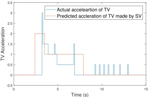
2.12 Predicted TV acceleration and actual TV acceleration. . . 31

2.13 Initial condition of Scenario II. . . 32

2.14 SV’s lane change intention being prevented by human driver. . . 32

2.15 SV’s final lane switch. . . 32

2.16 Vehicles’ velocities. . . 33

2.17 TV selection. . . 33

2.18 SV strategy. . . 34

3.2 Schematic diagram of DGTMPC. . . 38

3.3 The first game scenario. . . 43

3.4 The local naming of the differential game. . . 45

3.5 The second game scenario. . . 46

3.6 The switch logic of DGTMPC between mode 1 and mode 2. . . 48

3.7 TV’s MPC solution at each time step.. . . 60

3.8 Initial places of the vehicles in scenario I. . . 66

3.9 No.7 made a sudden lane change. . . 67

3.10 No. 5 start to decelerate after No.7’s sudden lane switch. . . 67

3.11 The estimation result of weights in No.5’s MPC, where its original weights are Qv=0.8,Ru=0.54Rh=0.27. . . 68

3.12 The estimation result of weights in No.5’s MPC, where its original weights are Qv=0.58,Ru=0.58Rh=0.58. . . 68

3.13 When SV has the opportunity to interact with No.5, he choose to stay in the current lane instead of doing lane change.. . . 69

3.14 SV and No.5 velocity profile. . . 70

3.15 SV’s lane change intention. 4s means SV does not want to change lane at all. . . 70

3.16 Weight estimation of No.5’s MPC cost function. . . 70

3.17 The GCV scope of DGTMPC. . . 71

3.18 When SV has the opportunity to interact with No.5, he choose to turn on the turning light. And No.5 responds to SV’s intention by opening a large gap. Then SV initiates a lane change. . . 72

3.19 SV completes the lane change and merge into the traffic in the upper lane. . . 72

3.20 SV and Ncyan vehicle velocity profile. . . 72

3.21 SV’s lane change intention. 4s means SV does not want to change lane at all. . . 72

3.22 Weight estimation of cyan vehicle’s MPC cost function. . . 73

3.24 The acceleration of No.5 in case 2 . . . 74

3.25 Vehicle initial positions in case 1. . . 75

3.26 First lane change of cyan vehicle. . . 76

3.27 Second lane change of cyan vehicle. . . 76

3.28 SV and cyan vehicle’s velocity profile. . . 77

3.29 TV’s lane change planning in the simulation. . . 77

3.30 Estimation result of cyan vehicle’s MPC weight . . . 78

3.31 Vehicle initial positions in case 2 . . . 78

3.32 Cyan vehicle made the first lane change . . . 79

3.33 Cyan vehicle interacts with SV and choose not to overtake SV . . . 79

3.34 Cyan vehicle changed lane after SV. . . 79

3.35 Two vehicles’ velocity in the simulation. . . 79

3.36 TV’s lane change planning in the simulation. . . 80

3.37 Estimation result of cyan vehicle’s MPC weight . . . 80

3.38 The average speed in each scenario of each controller. . . 84

3.39 DGTMPC’s decision under a specific scenario. . . 85

LIST OF TABLES

TABLE Page

1. INTRODUCTION AND LITERATURE REVIEW

1.1 Background and Objectives

The fact that governments, vehicle manufacturers and IT companies are spending billions of dollars in research and experiment of autonomous vehicles (AV) indicated AV has been considered a promising technology. The reason is that AV could bring multiple potential improvements to our society, including increased traffic safety, better environment, reduced utilization of manpower and so forth [1].

However, besides the advantages AV has, there remain some challenges we have to face. One of them is AV-human-driver interaction. As more AVs hit roads, we will soon face blended traffic situations that contain both autonomous, semi-autonomous and human-driven vehicles. Although safety is always of the top priority, a conservative setup in such a situation could lead to a some issues. First, the behavior of an excessively conservative vehicle might look weird from a human driver’s perspective. Second, in a blended traffic of both human driver and self-driving cars, human drivers would finally realize the overly-cautious characteristic of such an autonomous car and bully the car for more advantages during the interaction. Therefore, to smoothen the adaptation process, researchers must not only emphasize safety, but should also ensure that self-driving vehicles act in a human-like manner so as to behave consistently with ordinary driving norms [2, 3, 4].

Therefore, this study will proposed a category of AV motion controllers that can address the above issue in highway driving situation.

The controller will consist of two layers. The high level controller that makes strategic deci-sions and the low level control that controls the AV’s specific movements.

Based on kinematic information of both surrounding vehicles (SRV) and subject vehicle (SV), the high level controller should be able to make balanced decisions that consider both SV’s safety and driving advantage. Such decisions should be reasonable enough to be made by human drivers. This also indicates that a human-like decision should also includes advanced tasks like overtaking

or MLC, which would require that the high level decision maker should also consider the coordi-nation between longitudinal and lateral movement. In addition, such decision should consider the interaction between human driver and AV. In other words, the high level controller should be able to think from human drivers’ perspective and make movements based on their possible strategies.

The low level controller controls the longitudinal motion and lane change. Besides the ability to achieve the decision made by high level controller, the low level controller should also ensure a collision-free path.

1.2 Literature Review

1.2.1 Autonomous Vehicle Decision and Control

We do a thorough literature review on AV decision making and control technique in this section. The control approaches are divided into three categories in the following text: Separate control, coordinated control and planning-type approaches.

Separate control means controlling the longitudinal motion and lateral motion of the vehicle separately. Coordinated control indicates a certain level of cooperation between the lateral and lon-gitudinal motion. Therefore, the vehicle may perform more complicated behavior like overtaking by acceleration. Path planning approaches plans AV’s future path in advance, and a controller is responsible for tracking such path.

1.2.1.1 Longitudinal Control

In terms of longitudinal motion, there are several widely-used models. The General Motors model (or the GHR model) is proposed by Denos C. Gazis, et al. [5]. It was named after GM because it was estimated using data collected on GM test track. The collision avoidance model developed by Gipps is another famous model[6]. The advantage of this model is that it ensures a safety distance between the subject car and the front car, which the GM model fails to consider. Optimal velocity model [7], different from the previous two, is a dynamic model that suggests the car’s acceleration is proportional to its optimal speed and actual speed. The next widely-used car following model is the Intelligent Driver Model [8], which define the acceleration as a function of

velocity , net distance gap and the velocity difference in a way different from GM model.

Many other searchers are working on expanding the above model from single-regime to multi-ple ones. Ahmed considered the following two regimes for his acceleration model in [9]: free-flow regime and car-following regime. He also proposed a good way to evaluate parameters in his model according to real traffic data. Yang also considered emergency regime in MITSIM they established [10]. In [11], the paper includes three more regimes. ACC is another widely-studied driver assis-tance technique [12, 13] and many variants have been raised like Multi-Objective ACC[14, 15], Model Predictive ACC [16, 14], cooperative ACC [17, 18] etc.

Many other mature control methods has also been used for vehicle longitudinal control. Nou-veliere proposed a second-order sliding mode control scheme [19]. In [20, 21], Lyapunov direct methods are used for either linear model or nonlinear one.

1.2.1.2 Lateral Decision and Control

Different from vehicle’s longitudinal motion, vehicle’s lateral motion is sometimes considered discrete in terms of lanes. Thus researches either consider lane change process as a “decision” by ignoring the specific lateral movement or use models like “bicycle” model to control the vehicle’s lateral position continuously. Lateral control discussed in this section is only limited to steering control for regular lane change.

Rule-based lane change decision are widely accepted in papers especially those about micro-scopic traffic due to the large amount of vehicles in the simulation models. Lane change rule is generally based on gap acceptance in consideration of vehicles’ positions, velocities and accelera-tions.

A common way of designing rules is to categorize lane change into several types according to the urgency of lane change due to the fact that lane changes are usually classified into differ-ent types. Gipps and Hidas categorize lane changing into three types: “Essdiffer-ential” , “Desirable” and “Unnecessary” according to vehicle’s position to the end of the lane [22, 23]. Ahmed in his dissertation classifies lane change into MLC and DLC according to the purpose of lane change and includes a probabilistic framework before triggering the corresponding rule for each type [9].

The lane change behaviors in SUMO [24] are divided into three types. Strategic (mandatory) lane change, cooperative lane change and tactical (discretionary) lane change, which is a compound of predecessor’s work. In [25] the same longitudinal controller is used while MLC and DLC are dis-tinguished by critical gap acceptance analysis. References [26] and [27] all proposed their own way of integrating MLC and DLC in a microscopic traffic study. The former paper, in particular, pro-posed a vehicle automation and communication system, which controls the longitudinal motion as well as the lateral motion of all the individual vehicles in the system in order to achieve maximum traffic efficiency. A lane-change model that is compatible with a number of car-following models is illustrated in [28]. This lane change rule is also based on standard gap acceptance models. Other researchers consider categorization of lane change in a different way.

Besides gap acceptance, other researchers have set up the problem in a cooperative framework. Kesting thought of modelling lane change behavior in a cooperative way [28]. The rule aims to minimize braking of both the subject car and other vehicles induced by subject car’s lane change. In [29] and [30], the authors assumed that two vehicles use Vehicle to Vehicle (V2V) communication to complete the merging behavior cooperatively. Van Arem et al. [31] and Xu et al. [32] used cooperative adaptive cruise control along with V2V technology to achieve collaborative highway merging.

Researchers have also aimed to design controllers that target the precise control of one vehicle in a specific situation. These approaches usually control the steering wheel to track a reference obtained from certain path planners. Schildbach and Borrelli propose an MPC that can plan lane-change behaviors while taking into account the behavior of surrounding vehicles in [33]. In[34], [35] and [36], researchers presented several diversified optimal feedback controllers for vehicle’s steering wheel task. Other well-known methods include PID [37], fuzzy control [38] etc.

Intuitively safety plays a more important role in an MLC scenario as compared to DLC because there is limited time to make a decision before crashing into an obstacle or reaching the end of a merging area. The decision could be difficult if there are competing vehicles in the target lane. This requires that one simultaneously evaluate the possibility of entering any one of multiple gaps

instead of considering them sequentially, i.e., one at a time. Thus, designing an autonomous driving system that is capable of handling an MLC scenario effectively requires the balance of factors associated with safety and driving advantages, for example, driver’s desire for speed, headway or ideal lane, etc.

Despite many research results on lane changing, some points have been less adequately ad-dressed. Lane change is coordination between vehicle’s longitudinal and lateral control, thus lon-gitudinal controllers should serve to create a better lane-change opportunity. A Moreover, V2V technology is yet to be used in practice and competing vehicles in reality are not always cooper-ative. Therefore, cooperative control scheme needs to be fully validated under a non-cooperative scenario. In addition, human drivers (based on whose behavior lane change strategies are mod-elled) can actually consider several gaps in their adjacent lane(s) at the same time and choose one that typically optimizes safety and driving advantage. In other words, considering the human driver as a reference is likely of value in this context.

1.2.1.3 Coordinated Control

Generally approaches of coordinated control evaluates longitudinal and lateral motion in the same framework. Utility function is defined as a criterion to represent each decision’s advantage to AV.

Belleman introduced Markov Decision Process(MDP) to model systems that are not only con-trollable but also stochastic [39]. In MDP, the evolution of the system does not purely depends on transition probability but also on action. Brechtel et al. developed a discrete MDP model whose action space includes both longitudinal acceleration and lateral velocities for lane change and col-lision avoidance [40]. Coskun et al. proposed a fuzzy MDP model for mandatory lane change which allows AV to adjust its longitudinal velocity to fit the velocity of the main traffic stream while executing the MLC [41]. Li et al. illustrate a controller that integrates MPD and game theory. Counting in the interaction between vehicles and model uncertainty, the controller is able evaluate totally seven actions in both longitudinal and lateral direction[42].

category. It can not only predict surrounding vehicle’s behavior by considering their reaction to the subject vehicle, but also flexibly set up the game as needed, which means lateral movement, longitudinal movement or complicated movement can be considered simultaneously under the same criterion and coordination of longitudinal and lateral motion can be easily achieved. The detailed literature review of game theory is given in Section 1.2.2.

Hybrid system is an adequate method for modeling traffic because drivers intuitively consider lane selection as the discrete state and longitudinal position as continuous state [43, 44, 45]. Such feature enables researchers to consider different constraints or continuous dynamics that may be applicable in each discrete state.

1.2.1.4 Path Planning Approaches

Planning-type approaches generally includes two steps. Generating the path and tracking the path. The first step sets up a specific near-future path for the vehicle and the second step is con-trolling the vehicle to track the path. Usually these approaches’ contribution is in the first step while the second step can be achieved by well-known control techniques like PID, sliding mode, h-infinity and so forth.

Many popular path planning algorithms and their variant, like A*, D* [46, 47] are based on the cell decomposition algorithm. These methods decompose the environment into cells and the planner computes explicit robot motions within each cell. With several years evolvement, some variant of the above algorithms have been proposed. [48] described hybrid A* algorithm, which was validated in the DARPA Urban Challenge. The algorithm first obtain a kinematically feasible trajectory phase then improves the solution via numeric non-linear optimization.

Another category is sampling based approaches like probability Road Map (PRM) [49] and rapidly-exploring random tree (RRT) [50]. These approaches construct a set of collision-free tra-jectories at high efficiency due to its probabilistic feature. In Aoude’s papers, the author raised a new algorithm called RR-GP, which is a combination of RRT and Gaussian Process (GP). GP is responsible for obstacle movement prediction and RRT is responsible for feasible path generation. [51, 52] proposed an improved RRT and showed its application to the 2007 DARPA challenge. [53]

presented a new algorithm called Rapidly exploring Random Graph (RRG), and showed that the cost of the best path in the RRG converges to the optimum. [54] developed a game theoretic path planning method based on RRG for multi-robot motion planning problem. In [55, 56, 57], authors illustrated a sampling-based path planning algorithm called B-spline curves. Smooth-primitive constrained-optimization-based path-tracking algorithm.

Potential field method [58] assumes that robots moves in a field of forces. The position to be reached is an attractive pole and obstacles are repulsive surfaces. The control effort can then be easily obtained by summing up the attraction and repulsion. Gradient descending or Newton method are often used to find the optimal waypoint in the field [59].

The dynamics window approach [60, 61] forms the search space of trajectory by considering the dynamics of robots, specifically, the reachable velocities in a time scope.

State lattice [62, 63, 64] samples the state space regularly to generate the path, while taking into account the kinematic and dynamic constraints of the robot. [65, 66] showed their improved work so that the method can be used in more complicated environments with a frequently-varying dominant direction like urban areas. [67] applied the resolution-equivalent grid method to state lattice to solving the coupling between state variables induced by dynamic constraints at high speed.

1.2.1.5 End to End Control

Artificial neural networks can be considered an end to end control approach that is totally different from other. As long as enough training data is give, the networks can function as a controller that mimics the objects which we get the training data from. [68] proposed a deep-neural-network-based autonomous driving scheme. The system was trained in-real time with the training data generated from internal simulators and can intelligently estimate future behavior of surrounding vehicles. [69] demonstrated an autonomous driving system using NVIDIA Drive PX. Instead of decomposing problem into a series of tasks like lane marking detection, path planning, and control, their end-to-end system optimizes all processing steps simultaneously. The system was trained with driver’s activity data including lane keeping, lane change and so forth. IT showed

the trained network is able to finish a 10 mile driving task with little help from driver. 1.2.2 Game Theory

Game theory is the formal study of conflict and cooperation between rational agents. It provides researchers a mathematical language to model and to analyze scenarios where there exist strategic interactions.

Game theory has been applied in various ways to study the effects of policy, decisions, and the actions of individual agents in a transportation system. These studies can be broadly classified into two categories: infrastructural regulation studies (traffic control problem) and agent-oriented studies (vehicle placement or route decisions). In the first category, researchers have employed game theory in relation to dynamic traffic control or assignment problems. For instance, Chen and Ben-Akiva [70] adopted a non-cooperative game model to study the interaction between a traffic regulation system and traffic flow to optimally regulate the flow on a highway or an intersection while Zheng-Long and De-Wang [71] addressed the ramp-metering problem via Stackelberg game theory. Su et al. [72] have also used game theory to simulate the evolution of a traffic network.

In the second category, vehicles are regarded as game participants and traffic rules are generally considered to be implicit in the respective decision models [73, 74, 75]. In this context Kita [76] has worked to address the merging-giveaway interaction between a through car and a merging car as a two-person non-zero-sum game. This approach can be regarded as a game theoretic interpretation of Hidas’ driver courtesy scheme [77] from the viewpoint that the vehicles share the payoffs or heuristics of the lane-changing process. This leads to a reasonable traffic model although the approach does not address the uncertainties resulting from the actions of other drivers. In recent studies, Talebpour et al. [78, 79] have considered the notion of incomplete information as part of the game formulation process and have developed a model that in certain respects addresses the aforementioned concern. Likewise, Altendorf and Flemisch flow [80] have developed a game theoretic model that addresses the issue of risk-taking by drivers and its impact on the traffic flow. Their study focuses on the cognitive aspects of this decision making process and its impact on traffic safety. Likewise, M. Wang, et al. [81] have used a differential game based controller to

control a given vehicle’s car-following and lane-changing behavior while in [82], the authors have applied an Iterative Snow-Drift (ISD) game on cross-a-crossing scenario. In [83], Stackelberg game theory was used solve conflicts in shared space zones while in [84] the authors compared heavy vehicle and passenger car lane-changing maneuvers on arterial roads and freeways. Elvik [85] offers a rather complete review of related works in this area, albeit up to 2014. Meng et al. [86] integrate the idea of receding horizon of MPC with game theory and proposed a game theoretic solution to dynamic lane change situations with incomplete information.

As is shown above, diversified types of games have been applied to transpiration research. The most common one is modeling driver’s lane change or merging behavior via a non-cooperative simultaneous game and a pure Nash equilibrium [87, 88]. Others have considered mixed strategy Nash solutions for similar game theory schemes [89, 90, 91]. Recently, advanced game types such as grey game [92], incomplete information game [80, 93] and Stackelberg game [94, 95, 96, 97] are introduced. Differential games are games that concerns control of dynamic systems. One group of researchers proposed several differential-game-based vehicle control frameworks in [98, 81], from non-cooperative to cooperative approaches. Differential games are also increasingly used in related fields such as vehicle/robot formation control [99, 100].

1.2.3 Model Predictive Control

Model predictive control (MPC) is a widely-used control technique. The most important char-acteristic of MPC is its ability to determine a sequence of control inputs for the model over predic-tion horizon given the cost funcpredic-tion and constraints. However, only the first input of the sequence is applied to the model. The optimization problem is solved periodically using the latest information and the horizon recedes as time goes so MPC is also called receding horizon control [101].

Many researchers have employed MPC to endow autonomous vehicles prediction capability. MPC predicts the future behavior of a system over a finite time horizon and compute a sequence of optimal control inputs that minimizes a cost function, while ensuring satisfaction of given con-straints. Gao et al. proposed a nonlinear MPC, the cost function of which considers the distance of the subject vehicle to the obstacle so that MPC is able to generate and follow a collision-free

path[102]. In [103], Rosolia et al. proposed a non-convex MPC for autonomous vehicle, where the non-convexity lies in non-convex constraint of the MPC. To avoid the non-convexity, some people set up their models such that MPC controls only the longitudinal motion[104]. Others employed hybrid MPC by defining the lanes as the discrete state and longitudinal motion as continuous state, so that different constraints or continuous dynamics may be applied[44, 45].

Attempts of combining GT and MPC have been made in some papers. Na et al. proposed a linear quadratic game-based MPC for the control of active front steering system [105, 106]. Yoo et al. raised a collision avoidance technique where model predictive controller controls the vehicle to avoid the unsafe zone generated by the NE [90]. Distributed MPC is another topic on this specific cross-subject field [107, 108]. Despite some literature on this topic, little can be found in combining a non-cooperative game and MPC in a hierarchical way.

1.2.4 Driver Aggressiveness and Estimation

Human drivers’ strategies are largely dependent on their driving style. To accurately predict human drivers’ future behavior, an autonomous driving system should take into account other vehi-cles’ aggressiveness. However, there are mainly two challenges to achieving this. For one, there is no widely accepted definition for aggressive driving. Most published papers define this notation by driver’s self-evaluation in questionnaires [116, 117] or rely on observation of aggressive behaviors in field studies [118, 119]. For another thing, if vehicles are not connected, real-time estimation is almost the only way to identify a driver’s aggressiveness, but few published works exist on this subject.

Previous studies on aggressiveness estimation are almost always conducted offline and are based on field observation or questionnaires[120, 121, 122, 123]. These researches mainly study aggressiveness by considering frequency of aggressive behaviors, including honking a horn, tail-gating, swearing, forcing, etc., and statistically relate them to drivers’ features, like age or gender, statistically. However, these methods are difficult to use with an autonomous driving system for such data can generally only be collected and processed offline.

Drivers’ aggression are often divided into two or three types (conservative, neutral and aggressive) and each type of drivers has quantitatively distinct driving style. For instance, aggressive drivers prefer higher desired speed [124], larger acceleration, smaller following distance [125] when per-forming car following and larger weight on payoff and smaller weight on collision risk [95] when doing lane change. These papers usually suggest a statistic distribution of these types of drivers on the road and check their influence on the traffic.

In spite of a certain amount of research regarding driving aggressiveness, no published works have proposed a viable approach of estimating their quantity on-line.

1.3 Game Theory Basics

Game theory was systematically established by von Neumann and Oskar Morgenstern in 1944 [126]. Then John Nash introduced the famous Nash equilibrium in noncooperative game theory, at which none of the players can deviate from his own strategy and gain better payoff [127]. From then on, game theory has been applied to numerous fields including economic theory, engineering, sociology, psychology and so forth.

Game is the object of game theory and is a formal mathematical model of an interactive situa-tion. Generally, a game consists of the following elements:

• Player. Players are agents that are involved in the interaction • Sequence. Sequence is the order that agents play their strategy • Strategies. Strategies are actions a player can take

• Payoff. Payoff is the reward that a player can gain after every player plays his or her strategy • Level of cooperation. A game is either cooperative or non-cooperative. In cooperative game, players are optimizing the sum of their payoff. In non-cooperative one, each player is maxi-mizing their own payoff.

distribution, then information is incomplete. Then the players are trying to maximize the expected payoff.

• Equilibrium. Equilibrium is a pair of strategies (in order sometimes) that satisfies a set of predefined rules. Equilibria are not necessarily the Pareto optimal, but they generally reflect real human’s decision logic. There are many kinds of equilibria. Nash equilibrium, Stackelberg equilibrium, Correlated equilibrium, Sequential equilibrium and so on. They have different definitions and thus fit different kinds of interactions.

Stackelberg game was raised by Heinrich Freiherr von Stackelberg in 1943 [128]. The solution of a Stackelberg game is called Stackelberg equilibrium. Stackelberg game is a two-player sequen-tial game played by a leader and a follower. Here we refer to the leader as “him” and the follower as “her”. The leader first commits his strategy and the follower observes the leader’s strategy and responds with her own strategy. Each player is trying to maximize his/her own payoff. The leader in Stackelberg games is endowed the power of predicting follower’s strategy given his own.

The definition of Stackelberg Equilibrium is formally given in (1.1) to (1.2), where Lstands for leader,F stands for follower,aL andaF are leader’s and follower’s strategies, a∗L anda

∗ F are leader’s and follower’s optimal strategies,AL, AF are leader’s and follower’s strategy spaces,a∗L is follower’s optimal strategy set,ULandUF are leader’s and follower’s payoffs.

a∗_L = argmax aL∈AL min aF∈A∗F UL(aL, aL) (1.1) A∗_F(aL),{aF∗ ∈AF :UF(aL, a∗F)≥UF(aL, aF),∀aF ∈AF} (1.2)

For games of small scale in this paper, Stackelberg equilibrium can be found using exhaustive search, i.e., checking all possible joint strategies one by one.

1.4 Miscellaneous

This section includes some notes that helps readers better understand the main contents of the thesis.

1.4.1 Vehicle Naming

In this section we explain the naming of all the vehicles that appear in the thesis.

Figure 1.1: Vehicle naming

Fig.1.1 describes a classic highway driving situation. In the figure, the blue vehicle is the vehi-cle we control and we call itsubject vehicle(SV). All the orange vehicles are calledsurrounding vehicles(SRV).

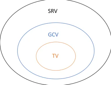
Intuitively, the control of SV only needs to consider a limited surrounding area to make deci-sion, so we define acandidate vehicle scopefor SV as a blue transparent area with green outline in Fig.1.1. The lateral range of the perception scope involves two adjacent lanes and SV’s current lane. All the SRVs in the scope are named game theoretic candidate vehicles (GCV). GCV is a candidate because SV considers entering the gap in front of GCV. For explanation purpose, we call the vehicle that is in front of a certain GCV preceding vehicle of that GCV (PV). The naming of GCV indicates that SV could interact with GCVs through games. Of all the GCVs, SV will finally choose at most one GCV as the target. And we call ittarget vehicle(TV). And the gap in front of TV istarget gap. The relationship between each different types of SRVs are shown in Fig. 1.2.

As a routine in game theory, we call SV ’he’ and call SRV/GCV/TV ’she’ for the convenience of explanation.

text, the same variables with subscript of “SRV”, “GCV” and “TV” share the same definition. We will use one of the three subscripts that best fits the role of that vehicle in that situation.

SRV

GCV

TV

Figure 1.2: Relationships between vehicle names.

1.4.2 Vehicle Kinematic Model

The simple kinematic model in this section is used throughout the whole dissertation. The longitudinal kinematic model of SV is given as (1.3).

   ˙ pSV(t) ˙ vSV(t)   =    1 0 0 1       pSV(t) vSV(t)   +    0 1   uSV(t) (1.3)

wherepSV,vSV anduSV are the longitudinal position, velocity and acceleration of SV respectively. For implementation in a simulation environment, we follow the the Euler method[129]. We introduce (1.4) to discretize the continuous state space.

whereTsis the sampling time.

Combining (1.4) and (1.3) gives us gives the discrete state-space form of SV’s kinematic model as (1.5).    pSV(k+ 1) vSV(k+ 1)   =    1 Ts 0 1       pSV(k) vSV(k)   +    0 Ts   uSV(k) (1.5)

wherek is the discrete time index.

For lateral movement of SV we simply assume the lane of SV is the discrete state for vehicle’s lateral movement. There is no continuous lateral motion.

For SRVs, we assume they have the exact same longitudinal and lateral model as SV. 1.4.3 Controllers of SV and SRV

In the model, there are two types of controllers: SV’s controller and SRV’s controller. SV always uses GTMPC. The controllers of SRV are different in each chapter and will be described at the beginning of each simulation section. The common feature of those SRV’s controllers in each chapter is that they can respond to SV’s strategy from a game theoretic approach.

1.5 Organization of the Dissertation

The dissertation will include two pieces of works.

Chapter 2 is about a game theoretic four-stage MPC (GT4SMPC). The chapter is organized as follows. In Section 2.1, the Stackelberg lane change game is clearly defined. In section 2.2, GT4SMPC is introduced. In Section 2.3, the platform is explained and simulations are given. In Section 2.4, conclusions are drawn.

Chapter 3 is about the DGTMPC. In Section 3.1 the structure of DGTMPC is introduced. In Section 3.3 the model of lane change differential game is explained. In Section 3.2, the process of using branch and bound algorithm to solve the Stackelberg differential game is shown. In Section 3.5, the IMPC algorithm is given and described. In Section 3.6, the controller is validated in simulation environment. In Section 3.7, conclusions are drawn.

2. GAME THEORETIC FOUR-STAGE MODEL PREDICTIVE CONTROL

In this chapter we proposed a game theoretic four-stage model predictive controller (GT4SMPC) for highway driving. The GT4SMPC has a two-layer structure. The high-level controller of GT4SMPC is a game theoretic decision model and the low-level controller is a model predic-tive controller (MPC). The high-level controller is responsible for decision making of surrounding vehicle (SRV). MPC in the lower level controller controls SV’s longitudinal motion and SV’s lane decision.

To make intelligent decisions on the highway, GT4SMPC constantly establishes and solves Stackelberg games corresponding to multiple game candidate vehicles (GCV). Such interaction is initiated by SV’s signaling a lane change intention through turning light or a small lateral move-ment. By selecting one target vehicle (TV) among multiple GCVs based on SV’s payoffs indicated by the Stackelberg equilibrium of the games, GT4SMPC is able to enter the gap in front of the TV. Satisfactory simulations results showed that the GT4SMPC can achieve intelligent highway driving in simulated dynamic traffic. To further validate the effectiveness GT4SMPC we also conducted a series of human-in-the-loop driving simulations. The experiment results showed the proposed GT4SMPC is able to interact with human driver intelligently.

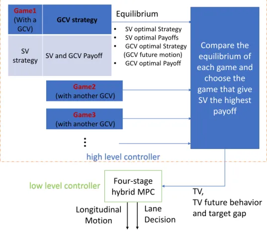
The schematic diagram of GT4SMPC is given in Fig.2.1.

The high-level controller is where all the games are established. It chooses the closest several vehicles in the game scope defined in Fig. 2.2 as GCVs. Then for each GCV, a game is established and solved to determine the optimal payoff of SV if SV choose to interact with that GCV. A simplified version of the low level MPC is used to generate SV’s payoff in the game given GCV’s strategy. We also define a payoff function for GCV based on its current headway and its desired speed, which is a function of both players’ strategies as well. Knowing all the payoffs of each strategy pair enables us to compute the solution of each game. Comparing the results of each game gives the optimal GCV for SV to interact with, i.e., TV, along with the target gap, both of which are fed to the low-level controller.

The low level controller is a four-stage hybrid model predictive controller, whose name comes from the four stages of the lane change process we define in this paper. Given the signals of the high-level controller, the low-level one is able to drive the vehicle to the desired position and initiate the lane change at the best moment.

Game1 (With a

GCV) GCV strategy

SV

strategy SV and GCV Payoff

Equilibrium • SV optimal Strategy • SV optimal Payoffs • GCV optimal Strategy (GCV future motion) • GCV optimal Payoff Four-stage hybrid MPC Longitudinal

Motion LaneDecision high level controller

TV,

TV future behavior and target gap

Game2 (with another GCV) Game3 (with another GCV)

…

choose the game that give

SV the highest payoff

low level controller

Figure 2.1: Controller schematic diagram.

2.1 Stackelber Game

We assume SV are playing games with GCVs during the lane change process. Here we target the Stackelberg equilibrium of the game because the interaction during the lane-change process can be simplified as a sequential game. SV plays its strategy first by switching on the turning

signal or slightly shifting towards the target lane, and GCV is assumed to respond to SV in a few seconds by possibly applying a different acceleration. The above sequential game is updated and played recursively for the duration of the interaction.

Stackelberg game was raised by Heinrich Freiherr von Stackelberg in 1943 [128]. The solution of a Stackelberg game is called Stackelberg equilibrium. Stackelberg game is a two-player sequen-tial game played by a leader and a follower. Here we refer to the leader as “him” and the follower as “her”. The leader first commits his strategy and the follower observes the leader’s strategy and responds with her own strategy. Each player is trying to maximize his/her own payoff. The leader in Stackelberg games is endowed the power of predicting follower’s strategy given his own.

The definition of Stackelberg equilibrium is given as (2.1)-(2.2).

a∗_L = argmax aL∈AL min aF∈A∗F UL(aL, aF) (2.1) A∗_F(aL),{aF∗ ∈AF :UF(aL, a∗F)≥UF(aL, aF),∀aF ∈AF} (2.2)

where a∗_L and a∗_F are the optimal strategies of leader and follower respectively, AL and AF are the strategy set of leader and follower,ULandUF are payoff functions of leader and follower. In this paper, as we have defined above, SV is the leader and GCV is the follower. Their payoffs are already given in (2.17) and (2.3). SV’s strategy set is all the possible valuesN₀0 can be, whereN₀0 is SV’s strategy. GCV’s strategy set includes all the possible accelerations that GCV can choose as well as instantaneous lane change to adjacent lanes.

According to [130], equilibrium of small-scale games like those in this paper can be easily found by checking all the possible solutions.

To fully define the lane-change Stackelber game, we need to define its players, and their strate-gies and payoffs.

2.1.1 Game Scope and Players

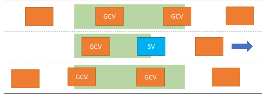
In Fig. 2.2, the game scope is defined as the green area. This indicates the assumption that SV is able to interact with every vehicles within that area and the possibility that SV could enter any

SV GCV

GCV GCV

GCV GCV

Figure 2.2: The green area is the game scope.

gap "guarded" by a vehicle in green area in adjacent lane. In addition, SV’s action also has some impact on the vehicle that follows him at any time, so we assume interaction between them too. All the vehicles in green area are called game candidate vehicle (GCV).

For each GCV and SV pair, we establish a two-player Stackelberg game between them. Thus in each game, the players are SV and one GCV. We assume SV is the leader in the game for two reasons. First, if SV initiates a lane change, it is more reasonable to define SV as the leader. Second, we do not want our SV just passively react to the traffic but actively pursue advantages. For more details of the Stackelberg game, readers may refer to [130].

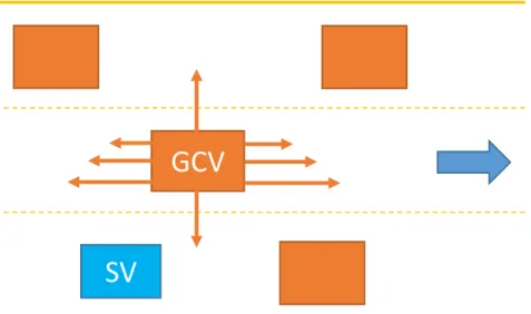
2.1.2 GCV Strategies and Payoffs

In our set-up, we assume the GCV is able to move in four directions as her response to SV in the game. To be specific, we define several longitudinal accelerations and instantaneous lane switch as GCV’s strategy (Fig. 2.3).

GCV’s payoff is defined as (2.3). UGCV(k) = N X k=1 (Upos(k) +Uvel(k)) (2.3)

SV

GCV

Figure 2.3: GCV strategy space.

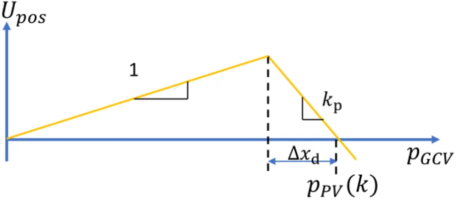
where Upos(k) =        pGCV(k), if∆p(k)≥∆pd pP V(k) + (kp −1)∆pd−kp∆p(k), if∆p(k)<∆pd (2.4) Uvel(k) = kv|vd−vGCV(k)| (2.5) ∆p(k) =pP V(k)−pGCV(k) (2.6)

In (2.3) to (2.6),Upos is the position part of the payoff, Uvel is the velocity part of the payoff, pGCV is the longitudinal position of GCV,vGCV is GCV’s velocity,vdis GCV’s desired speed, PV is the preceding vehicle of GCV after all players play their strategies,pP V is the PV’s longitudinal position,∆p(k)is GCV’s current space headway,∆pdis GCV’s desired space headway,kpandkv are two negative parameters relating to the two parts of the payoff function.

The integration form of (2.3) indicates that GCV is considering the benefit of both spacing and velocity over the prediction horizon like SV. Equation (2.4) means that GCV wants not only to be as close to her destination as possible, but also to maintain safe distance by keeping desired space

𝑘

Δ𝑥

𝑝

𝑈

1

𝑝

(𝑘)

Figure 2.4: The position part of GCV’s payoff function.

headway from any PV. Equation (2.5) is GCV’s desire for the ideal speed. The position part of GCV’s payoff function can be drawn as Fig. 2.4.

Which vehicle is PV really depends on two players’ strategies. If GCV changes lane, then SV is assumed to change lane successfully and GCV’s new preceding vehicle becomes PV. If GCV does not change lane, then the new PV could be SV if SV changes lane successfully or the original PV if SV fails. This reflects the interaction between two players of the game.

2.2 The Four-Stage MPC, SV Strategies and Payoffs

In this section, we introduce the so called four-state MPC and talk about how we define SV’s strategies and payoffs in the game.

First, we would like to divide the lane change process of SV into four stages: 1. Traveling in the current lane. (TCL)

2. Leaving current lane. (LCL) 3. Crossing lane marking. (CLM) 4. Traveling in the target lane. (TTL)

Such classification is for pure control purpose in terms of constraints handling as well as lon-gitudinal and lateral control coordination.

While in TCL or LCL stage, SV is assumed to only consider the constraints associated with current lane. When in CLM stage, SV should pay heed to constraints of both lanes. When SV arrives at TTL stage, only constraints related to target lane needs attention.

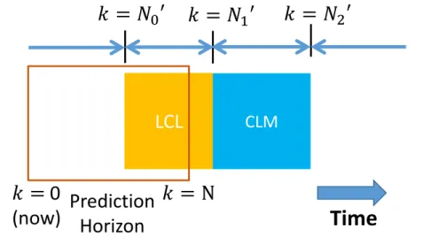
To better understand the role each stage plays in MPC, we draw Fig. 2.5. In the figure, the red rectangle is the prediction horizon. As time goes, it gradually moves towards the right side. N₀0, N₁0 andN₂0 are certain steps symbolizing the borders of adjacent stages in the prediction horizon if the horizon covers that border.

N₀0 will not show in the MPC cost function, because the purpose of LCL stage is to help GT4SMPC plan the best moment to start the lateral movement of the lane switch process. Such signal is sent to the steering controller so that the predicted moment when SV crosses lane marking, which is computed by MPC, matches SV’s actual lateral motion, over which GT4SMPC does not have full control.

For simplicity,N₁0−N₀0 andN₂0−N₁0 are fixed during the process of solving the MPC problem. Therefore for a certain game happening at a certain simulation step,N₀0,N₁0 andN₂0 are dependent. If one of them is determined, then all of them are. In reality, N₁0 −N₀0 and N₂0 −N₁0 can vary depending on how fast SV plans to execute the lane change. Such variation can be directly applied to the current controller, but consequently it produces extra computation load because of a larger strategy space of SV.

Based on the definition of the four stages, the four-stage hybrid MPC is proposed as (2.7). Please notice that the MPC is for both payoff generation of the game in high level and the control of SV’s motion in low level.

Time

LCL

𝑘𝑘

=

𝑁𝑁

′

𝑘𝑘

=

𝑁𝑁

′

CLM

𝑘𝑘

=

𝑁𝑁

′

TCL

TTL

Prediction

Horizon

𝑘𝑘

=

0

(now)

𝑘𝑘

= N

Figure 2.5: The four stages of lane change in MPC.

J(v, u, h1, h2, N10, N 0 2) = N₁0 X k=1 (Qv|v(k)−vdes|2+Ru|u(k)|2+Rh1|h1(k)|2) + N0 2 X k=N₁0+1 (Qv|v(k)−vdes|2+Ru|u(k)|2 +Rh1|h1(k)|2+Rh2|h2(k)|2) + N X k=N20+1 (Qv|v(k)−vdes|2+Ru|u(k)|2+Rh2|h2(k)|2) +QvN|v(N)−vdes|2 (2.7)

subject to

v(k)≥0 (2.8)

umin ≤u(k)≤umax (2.9)

∆umin ≤u(k)−u(k−1)≤∆umax (2.10)

h1(k)≥0 (2.11) h2(k)≥0 (2.12) for0≤k ≤N₂0 p(k)< h1(k) +pCP V(k) (2.13) p(k)> h1(k) +pCF V(k) (2.14) forN₁0 + 1≤k ≤N p(k)< h2(k) +pP P V(k) (2.15) p(k)> h2(k) +pGCV(k) (2.16)

whereN is the prediction horizon,u(k)is SV’s longitudinal acceleration, i.e., a control variable. h1(k) and h2(k) are two slack variables in constraints, vdes is SV’s desired velocity, Qv is the weight on the desired speed of SV, QvN is the weight on the terminal term, Ru, Rh1 and Rh2

are the weights on u, h1 andh2 respectively,umax andumin are the upper and lower bound of u. ∆umaxand∆umin are the bounds ofu(k)−u(k−1). PPV, CFV and CPV are just local naming of surrounding vehicles in terms of a specific GCV according to Fig. 2.6.

The second row of (2.7) is SV’s cost in TCL and LCL stages, the third and forth rows are his cost in CLM stage, and the fifth row is his cost in TTL stage and the last row is the terminal cost. Simply speaking, in all stages, SV cares about both speed and control effort, i.e., acceleration. In

SV

PPV GCV

CPV CFV

Figure 2.6: The local naming of MPC formulation.

TCL and LCL stages, SV tries to minimize the slack variable associated to the safety concern in current lane. In TTL stage, SV is minimizing that of the target lane. In CLM stage, SV cares about both. The meanings of constraints (2.8) to (2.12) are self-evident. (2.13) and (2.14) are the soft constraints that help SV keep distance from preceding and following vehicles in the current lane, whose slack variables also appear in (2.7). Similarly, (2.15) and (2.16) are the safety constraints associated with the target lane.

We need to point out that (2.7) is abused here. IfN₁0 orN₂0 is not in the prediction horizon, then corresponding row will not appear in the cost function .

From (2.7) we can see that GCV’s strategy is also influencing SV’s trajectory planning in the game. Here we use a linear decreasing acceleration model in[131] as SV’s prediction of GCV’s fu-ture motion in SV’s game if GCV’s strategy is certain longitudinal acceleration. If GCV’s startegy is lane change, then we assume lane change is completely immediate and GCV follows constant velocity.

Given the MPC, we simply define the payoff function of SV as (2.17).

USV =−J (2.17)

In addition, since we know thatN₀0,N₁0 andN₂0 are dependent, any one of them can be consid-ered as SV’s strategy of the game.

2.3 Simulations

In this section, we validate GT4SMPC’s performance in two scenarios.

The first scenario is a normal highway driving situation. SV is trying to achieve high speed in a comparatively slow traffic by competing with traffic vehicles. All the traffic vehicles are controlled by a linear decreasing acceleration game theoretic controller (LDAGTC).

In the second scenario, we test GT4SMPC in a mandatory lane change scenario. The blue vehicle is controlled by a human in real time. The human will intentionally prevent SV from lane change so that we can observe how GT4SMPC behaves in such an extreme case. The black vehicles are still controlled by LDAGTC.

LDAGTC is a linear-decreasing-acceleration-model-based controller that can respond to SV’s lane change intention in a game theoretic way. According to the definition of Stackelberg game, a follower, which is a traffic vehicle controlled by LDAGTC in the simulation, does not predict the action of leader (SV), but passively observes it and makes the corresponding response. Therefore, a traffic vehicle actually does not need to establish a game of her own. She only observes SV’s current state, and infer SV’s strategy and his trajectory in a certain way. Here we assume LDAGTC uses constant acceleration model to predict SV’s future motion, and a lane-change rule based on gap acceptance to determine how soon SV is going to execute the lane change. Then LDAGTC will choose certain acceleration to either prevent SV’s lane change intention or yield to SV as long as that acceleration maximizes her payoff. Here, we still use (2.3) as traffic vehicle’s payoff function. One main concern for the simulations is information completeness. According to the text above, SV and traffic vehicles share follower’s payoff function, follower’s model and the current states of all vehicles, but we also assume traffic vehicles do not know SV’s strategy or MPC’s trajectory and has to infer them. Such assumption brings uncertainty to the game: traffic vehi-cle’s actual behaviors might be different from SV’s prediction. Therefore, the information of the simulation is incomplete. In addition, we let human control a traffic vehicle in Scenario II. Since GT4SMPC can by no means know a human’s model or his/her payoff function, it could prove GT4SMPC’s performance and robustness in situations where traffic vehicles’ model is completely

unknown.

In both simulations, the high level of the controller is operated at 2Hz and the low level is operated at 5Hz. This means if the high level is not updated since its last activity, the low level will continue using the previous result of the high level. In high level the prediction horizonN is 4 steps, in low level it is 20. The prediction time is always 4s. The selection of these parameters is a result of balancing MPC’s speed and performance. A shorter prediction time undermines MPC’s motivation of lane change while a longer one involves too much future uncertainty. The selected frequencies make sure GT4SMPC can well handle the dynamic traffic in real time.

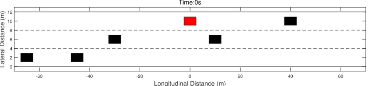
2.3.1 Scenario I

Multiple vehicles are traveling rightward on a three-lane road (Fig. 2.7). The red vehicle (SV) is controlled by GT4SMPC. Black vehicles, each of which is given a number for the convenience of explanation, are controlled by LDAGTC. There are two black vehicles in each lane. No.1 (right one, not shown in Fig. 2.7) and No.2 (left one) are traveling in the upper lane at 10m/s, No.3 (right one) and No.4 (left one) are traveling in the middle lane at 15m/s. No.5 (right one) and No.6 (left one) are traveling in the lower lane at 20m/s. SV starts at 10m/s and wants to achieve high speed in such a traffic. -60 -40 -20 0 20 40 60 Longitudinal Distance (m) 0 2 4 6 8 10 12 Lateral Distance (m) Time:0s

Figure 2.7: Initial condition of Scenario I.

Fig. 2.7 to Fig. 2.9 shows how SV made two consecutive lane changes to reach the desired speed.

0 20 40 60 80 100 120 Longitudinal Distance (m) 0 2 4 6 8 10 12 Lateral Distance (m) Time:5.3s

Figure 2.8: SV’s first lane switch.

120 140 160 180 200 220 240 Longitudinal Distance (m) 0 2 4 6 8 10 12 Lateral Distance (m) Time:12.1s

Figure 2.9: SV’s second lane switch.

According to the game scope that we have defined in Fig. 2.2, SV is constantly observing the surrounding gaps. At the beginning, since the vehicles in the top lane are slow and those in the middle lane are faster, SV would be willing to enter the middle lane. Thus SV chose No.4 to interact with (Fig. 2.11). By predicting No.4’s future behavior in a game theoretic way, SV thought that No.4 would accelerate mildly , which is indeed close to No.4’s actual acceleration (Fig. 2.12). Thus, SV plans a lane change between t=3.8s and t=7s as is shown in Fig. 2.10. The lines ofN₀0,N₁0 andN₂0 in the figure divide each lane change into the four stages. According to the definition ofN₀0,N₁0 andN₂0, SV is in TCL stage between t=0s and t=3.8s, in LCL stage between t=3.8s and t=5s, in CLM stage between t=5s and t=7s and in TTL stage after t=7s. This is how SV went through the four stages during the lane change.

Similar to the first lane change, SV attempted the second lane change after entering the middle lane and seeing the higher speed of vehicles in the bottom lane. This time SV predicts that the new TV No.6 is likely to maintain speed in the game. According to Fig. 2.12, No.4’s real behavior is

almost the same as SV prediction. Then SV accomplished the lane change between t=10.2s and t=13.6s. 0 5 10 15 Time (s) -2 -1 0 1 2 3 4 5 6 SV strategy (s) N₀' N₁' N₂' Figure 2.10: SV strategy. 0 5 10 15 Time (s) 0 2 4 6 TV number Figure 2.11: TV selection.

0 5 10 15 Time (s) -0.5 0 0.5 1 1.5 2 2.5 3 3.5 TV Acceleration Actual acceleartion of TV

Predicted accleration of TV made by SV

Figure 2.12: Predicted TV acceleration and actual TV acceleration.

change lane in order to make SV’s life more difficult. 2.3.2 Scenario II

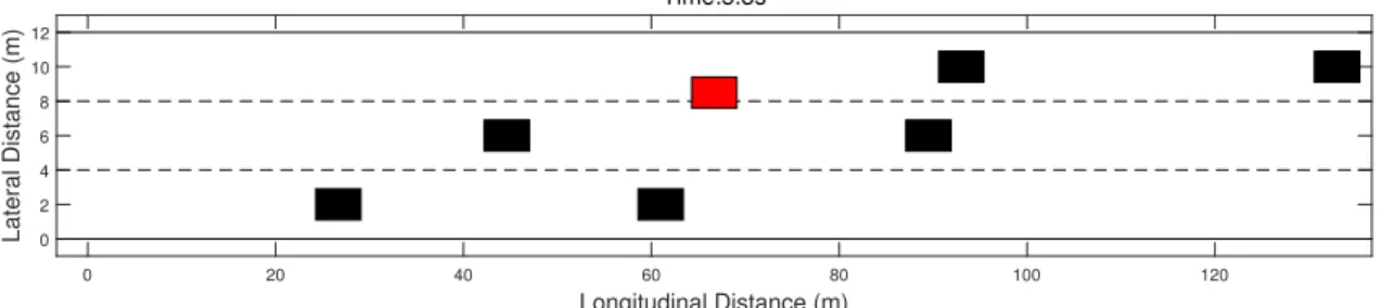
Now we would like to test GT4SMPC’s performance at the presence of human driver. We build a driver interface in MATLAB SIMULINK environment so that human can control the blue vehicle on the road in Fig. 2.13. During the simulation, the human driver can use the left and right arrows on the keyboard to adjust the blue vehicle’s longitudinal velocity and use the up and down arrows to select her desired lane. A built-in lateral controller will drive the blue vehicle into the target lane. In addition, this scenario is also designed to show GT4SMPC’s capability of running in real time.

We set up a scenario as Fig. 2.13. The red vehicle (SV) is still controlled by GT4SMPC and wants to achieve higher speed. The blue vehicle (No.4) is controlled by a human. The black vehicles use LDAGTC. The black vehicles in the lower lane have high desired speed (20 m/s), where the left one is No.3 and the right one is No.2. Working as an obstacle, another black vehicle (No.1) is traveling slowly (5 m/s) in front of the red vehicle, which is shown in Fig. 2.14. During the simulation, the human vehicle will intentionally prevent the red vehicle from lane change.

-60 -40 -20 0 20 40 60 Longitudinal Distance (m) 0 2 4 6 8 Lateral Distance (m) Time:0s

Figure 2.13: Initial condition of Scenario II.

40 60 80 100 120 140 160 Longitudinal Distance (m) 0 2 4 6 8 Lateral Distance (m) Time:6.1s

Figure 2.14: SV’s lane change intention being prevented by human driver.

60 80 100 120 140 160 180 Longitudinal Distance (m) 0 2 4 6 8 Lateral Distance (m) Time:11.9s

0 5 10 15 Time (s) 0 5 10 15 20 25 30 Velocity (m/s) No.1 No.2 No.3 Human(No.4) SV

Figure 2.16: Vehicles’ velocities.

0 5 10 15 Time (s) -1 0 1 2 3 4 5 TV number Figure 2.17: TV selection.

0 5 10 15

Time (s)

SV strategy (s)

N

'

N

'

N

'

According to Fig. 2.13 to Fig. 2.16, as SV was approaching No.1, the human vehicle was decelerating and trying to block SV. Targeting either No.3 or No.4 during t=0s to t=6s (Fig. 2.17), GT4SMPC was always planning a lane change in the near future andN₀0 even hit 0 occasionally, which triggered the lane change, but the lane change was then aborted after GT4SMPC’s awareness of human driver’s hostile behavior, according to Fig. 2.18. Therefore, SV kept staying in the merging lane and was not able to overtake the human driver at all before t=6s.

After human driver started accelerating after t=6s, No.3 also began to accelerate to prevent SV’s lane change intention, securing her position advantage. Taking this into consideration, SV continued selecting the current lane as the target lane until No.3 passed SV at around t=9s. Then SV decided to tug behind No.3 and completed the lane change according to Fig. 2.18. In Fig. 2.17, the fact that TV became 0 after t=6s means that SV was not trying to overtake any vehicle anymore.

indeed a heavy task for the high level controller and it takes MATLAB about 0.3s to get the result, so we set the game frequency at 2Hz, which is an acceptable value if we consider human driver’s frequency of decision making. The low level controller can actually run as fast as 20Hz, but we still let it run at 5Hz, which is fast enough for our simulations.

The two simulations showed GT4SMPC’s performance in different cases. Scenario I proved GT4SMPC’s ability of predicting surrounding vehicle’s behavior in a game theoretic situation. Scenario II showed GT4SMPC’s robustness in an extreme situation created by human driver. 2.4 Conclusion

The chapter proposed a novel game theoretic model predictive controller for autonomous high-way driving. The four-stage MPC divides lane change process into four stages of different con-straints, forming a hybrid MPC. With the help of game theory, the controller takes the possible response of traffic vehicles into account and is able to make rational decisions in dynamic traf-fics. Two simulations demonstrated GT4SMPC’s decent performance without knowing the exact model of surrounding vehicles. Since this piece of work is based on vehicle kinematic model, future works include testing the controller on vehicle dynamic models and using a driving sim-ulator to study the interaction between GT4SMPC and human drivers in a virtual while realistic environment.

However, the GT4SMPC also has two biggest drawbacks. First, the GCV model is assumed to play a fixed strategy during the prediction horizon. We wish that the GCVs in our model could make a sequence of decisions during their prediction horizons. Second, we have assumed fixed payoff function for GCV, which means in our simulations all the drivers are assumed to be exactly the same. In real life, however, drivers are different and it’s not reasonable to use the same payoff function to represent all the GCVs.

3. DIFFERENTIAL GAME THEORETIC MODEL PREDICTIVE CONTROL

In this section we propose a differential game theoretic model predictive controller (DGTMPC) for autonomous driving. The motivation of the new controller mainly comes from the weaknesses of the GT4SMPC: the fixed strategy and the fixed payoff function of GCV.

We consider the fixed strategy assumption over the prediction horizon unrealistic because in real life drivers are able to make a series of decisions (like Fig.3.1) when necessary. For instance, for a driver yielding to a another vehicle cutting in front of her, she could plan a strategy like this: decelerate to create a big gap and then accelerate to achieve the original speed. In spite of the simplicity of the strategy, the previous GT4SMPC did not include such decision sequence for GCV at all. Therefore, in our new DGTMPC we assume two players are playing a Stackelgerg differential game where each player is able to make a decision at each step of theN-step game , whereN is the prediction horizon.

The fixed payoff function is another unrealistic assumption for the GT4SMPC as well as for almost all researches that model traffic via a game theory approach. In literatures, parameters that are related to driving style in the game theoretic model are mainly determined in two ways. The first one is using values directly given by authors[132, 42, 80]. The first approach is groundless since authors do not give enough support for choosing such values. The second one is off-line calibration [93, 133, 134, 135]. In this category, researches use real drivers’ data from on-line database or experiments to calibrate parameters in the payoff functions. This approach seems solid but actually the calibration result only reflects the average driving style of the drivers in the data set or only a small bulk of the drivers involved in the experiment.

Targeting the above two issues, the DGTMPC in this section considers a much larger action space for the GCV in the game and uses inverse MPC to capture a specific driver’s feature through on-board observation.