LSHTM Research Online
Gabrio, A; Mason, Alexina; Baio, G; (2018) A full Bayesian model to handle structural ones and missingness in economic evaluations from individuallevel data. Statistics in Medicine. ISSN 0277-6715 DOI: https://doi.org/10.1002/sim.8045
Downloaded from: http://researchonline.lshtm.ac.uk/id/eprint/4650281/
DOI:https://doi.org/10.1002/sim.8045
Usage Guidelines:
Please refer to usage guidelines at https://researchonline.lshtm.ac.uk/policies.html or alternatively contact [email protected].
DOI: xxx/xxxx
ARTICLE TYPE
A Full Bayesian Model to Handle Structural Ones and
Missingness in Economic Evaluations from Individual-Level Data
Andrea Gabrio*
1| Alexina J. Mason
2| Gianluca Baio
11Department of Statistical Science, University College London, London, UK 2Department of Health Services Research and Policy, London School of Hygiene and Tropical Medicine, London, UK
Correspondence
*Andrea Gabrio, Corresponding address. Email: [email protected]
Present Address
Gower Street, London WC1E 6BT UK
Abstract
Economic evaluations from individual-level data are an important component of the process of technology appraisal, with a view to informing resource allocation decisions. A critical problem in these analyses is that both effectiveness and cost data typically present some complexity (e.g. non normality, spikes and missingness) that should be addressed using appropriate methods. However, in routine analyses, standardised approaches are typically used, possibly leading to biased inferences. We present a general Bayesian framework that can handle the complexity. We show the benefits of using our approach with a motivating example, the MenSS trial, for which there are spikes at one in the effectiveness and missingness in both outcomes. We contrast a set of increasingly complex models and perform sensitivity analysis to assess the robustness of the conclusions to a range of plausible missingness assump-tions. We demonstrate the flexibility of our approach with a second example, the PBS trial, and extend the framework to accommodate the characteristics of the data in this study.
This paper highlights the importance of adopting a comprehensive modelling approach to economic evaluations and the strategic advantages of building these complex models within a Bayesian framework.
KEYWORDS:
Missing Data; Bayesian Statistics; Economic Evaluations; Hurdle Models
1
INTRODUCTION
Economic evaluation alongside Randomised Clinical Trials (RCTs) is an important and increasingly popular component of the process of technology appraisal.1The typical analysis of individual level data involves the comparison of two interventions for which suitable measures of clinical benefits and costs are observed on each patient enrolled in the trial, often at different time points throughout the follow up. For simplicity, we generically term the clinical benefits as “effectiveness” and thus indicate the economic outcome variables as(𝑒, 𝑐).
Typically, effectiveness is measured through multi-attribute utility instruments (e.g. the EQ-5D 3L: http://www.euroqol.org), the costs are obtained using clinic resource use records and both are summarised into cross-sectional quantities, e.g. Quality Adjusted Life Years (QALYs). The main objective of the economic analysis is to combine the population average effectiveness and costs and use the precepts of decision theory to determine the most “cost-effective” intervention, given current evidence, as well as to assess the uncertainty in the decision-making process, induced by the uncertainty in the model inputs.2,3,4,5,6,7,8,9,10
In routine analyses, trial-based Cost-Effectiveness Analyses (CEAs) are usually performed under a frequentist approach in which the two outcome variables(𝑒, 𝑐)are modelled independently. Baseline adjustments are often included in the model using simple regression analyses.11,12,13This, often implicitly, assumes normality for the underlying cost and effectiveness data, or at least that the sample size is large enough for the means to be (approximately) normally distributed. In addition, almost invariably the relationship between the outcomes and the baseline characteristics is assumed to be linear.
There are several potential issues with this setting: firstly, the assumption of independence between costs and effectiveness is often questionable. While this is a recognised problem in the CEA literature, particularly under a Bayesian framework,7,14,15and although it may introduce bias in the statistical modelling and,a fortiori, in the economic evaluation,14,16appropriate methods to deal with correlation have historically found little application in routine analyses.17
Secondly, because both costs and effectiveness are usually characterised by a large degree of skewness, the assumption of normality is unlikely to hold and alternative approaches have been proposed in the literature. Examples include nonparametric bootstrapping18 and, particularly within a Bayesian approach, the use of more appropriate parametric modelling.15,16 Non-parametric bootstrapping mostly relies on using simple averages that often give similar results to those assuming normality.19 Conversely, modelling based on different parametric distributions (e.g. Gamma for the costs and Beta for the QALYs) often allows improvement in the model fit to the observed data and appropriately captures skewness.
Thirdly, data may exhibit spikes at one or both of the boundaries of the range for the underlying distribution. For example, some patients in a trial may not accrue any cost at all (i.e.𝑐𝑖= 0), thus invalidating the assumptions for the Gamma distribution, which is defined on the range (0,+∞). Similarly, we may observe individuals who are associated with perfect health, i.e. unit QALY,20 which makes it difficult to use a Beta distribution, defined on the open interval(0,1). A simple solution is to add/subtract a small constant𝜖to the entire set of observed values for the cost/effectiveness variable, thus artificially re-scaling it in the desired interval.21Despite being very easy to implement, this strategy is potentially problematic as the results are likely to be strongly affected by the actual choice of the scaling parameter𝜖and no clear guideline exists about the value to use (e.g.0.1,0.01,…). In addition, when the proportion of these values is substantial, they may induce high skewness in the data and the application of simple methods may lead to biased inferences.22 A more efficient solution suggested to handle this issue is the application ofhurdle models.22,23,24These are mixture models defined by two components: the first one is a mass distribution at the spike, while the second is a parametric model applied to the natural range of the relevant variable. Usually, a logistic regression is used to estimate the probability of incurring a “structural” value (e.g. 0 for the costs, or 1 for the QALYs); this is then used to weight the mean of the “non-structural” values estimated in the second component. Hurdle models have been discussed and applied in CEA mainly for handling structural zero costs.24,25,26
Finally, individual level data from RCTs are almost invariably affected by the problem of missing data. Numerous methods are available for handling missingness in the wider statistical literature, each relying on specific assumptions whose validity must be assessed on a case-by-case basis. Whilst some guidelines exist for performing CEAs in the presence of missing outcome values,27 they tend not to be consistently followed in published studies.28,29,30,31Analyses that are limited to the observed data (Complete Case Analysis, CCA) are inefficient and may yield biased inferences.26,32,33,34Multiple Imputation (MI)35 is a more flexible method, which increasingly represents thede factostandard in clinical studies.36,37 In a nutshell, MI proceeds by replacing each missing data point with a value simulated from a suitable model.𝑀complete (i.e. without missing data) replicates of the original dataset are thus created, each of which is then analysed separately using standard methods. The individual estimates are pooled using meta-analytic tools such asRubin’s rules,35to reflect the inherent uncertainty in imputing the missing values. For historical reasons, as well as on the basis of theoretical considerations, the number of replicated datesets𝑀is usually in the range 5-10. 35,38,39
As a consequence of the separation between the imputation and the analysis steps, MI requires the property of congenial-ity, i.e. the imputation model needs to be specified as equally or less restrictive than the analysis model. 40In addition, in many applications, MI is based upon assuming aMissing At Random(MAR) mechanism, i.e. the observed data can explain fully the reason for why some observations are missing. However, this may not be reasonable in practice (e.g. for self-reported ques-tionnaire data) and it is important to explore whether the resulting inferences are robust to a range of plausibleMissing Not At Random(MNAR) mechanisms, which cannot be explained fully by the observed data. Neither MAR nor MNAR assumptions can be tested using the available data alone and thus it is crucial to perform sensitivity analysis to explore how variations in assumptions about the missing values impact the results.41,42
Building on the existent literature, we show how models that simultaneously account for different potential sources of bias can be efficiently specified under a full Bayesian parametric framework, which has several advantages in comparison to a frequentist counterpart, specifically in health care technology assessments.7,10Firstly, by virtue of its modular nature, Bayesian modelling
is very flexible, which means that a basic structure can be relatively easily extended to account for the increasing complexity required to formally allow for the several features described above. We exploit this in §3. In addition, the Bayesian approach naturally allows for the principled incorporation of external evidence (e.g. expert opinions) through the use of prior distributions. This is often crucial for conducting sensitivity analysis to a plausible range of missingness assumptions including MNAR43,44, particularly when the evidence produced by the current study is limited, as is the case for small pilot trials, whose objective is to aid decision making about larger investments. Examples include the conduct of a full-scale trial, or the introduction in the market of a new cancer drug, based on the extrapolation of survival data produced over a short follow up.
Moreover, we note that MI can be considered as an approximation to a full Bayesian analysis on different levels. First, MI separates the imputation and analysis steps in two estimation procedures while, within a full Bayesian approach, the parameters of interest are estimated simultaneously with the imputation of the missing values and no additional analysis orad hocpooling is necessary. Even though it has been shown that MI performs well in most standard situations, when the complexity of the analysis increases, a full Bayesian approach is likely to be a preferable option as it naturally allows the propagation of uncertainty to the wider economic model and to perform sensitivity analysis. Second, due to the small number of replicates that are kept in practice, MI can be thought of as a fully Bayesian analysis based on a few simulations. Interestingly, the often-quoted objection to Bayesian modelling, i.e. that it is too computationally intensive in comparison to simpler frequentist counterparts, is likely to dissolve in the presence of extremely complex models, which would require tailor-made routines for the optimisation of non-standard multivariate likelihood functions, thus effectively surrendering their computational advantage over intensive but efficient sampling methods such as Markov Chain Monte Carlo (MCMC).
The main contribution of this work is to provide a unified framework that allows jointly tackling the features in CEA discussed above. We use a real case study based on a small pilot trial as our motivating example. Starting from the original analysis, we progressively expand our basic model. We specifically focus on appropriately modelling spikes at the boundary and missingness, as they have substantial implications in terms of inferences and, crucially, cost-effectiveness results. We then use another case study to show the flexibility of our approach and accommodate the specific characteristics of the data in this second trial.
The paper is structured as follows: in §2 we present the case study used as motivating example and describe the data. §3 defines the general structure of the statistical model used in the analyses and how it can be tailored to deal with the different features affecting the data. Initially, for simplicity, we present each model under a complete case scenario that will then be extended to account for missingness. §4 compares the results from three alternative models under both a complete cases and all cases scenario assuming MAR. The robustness of the results to alternative MNAR assumptions is then explored. §5 summarises the inferences for each model from a decision-maker perspective and compares their implications in terms of cost-effectiveness. §6 presents the second case study, the models used in the analysis and summarises the results of the economic evaluation. §7 discusses the proposed framework and suggests some improvements for future work. Finally, the Appendix includes additional material related to model assessment and the computer code for our analysis.
2
MOTIVATING EXAMPLE: THE MENSS TRIAL
We use as a motivating example the MenSS trial,45 a pilot RCT conducted in the UK public care sector to evaluate the cost-effectiveness of a new interactive digital intervention (the Men’s Safer Sex website, MenSS). This new intervention provides individually tailored advice on barriers to condom use to reduce the incidence of Sexually Transmitted Infections (STIs) in young men. A total of 159 men aged 16 years and over with female sexual partners and recent unprotected sex or suspected acute STI were recruited from three English sexual health clinics. Participants were randomised to receive either usual clinical care only (comparator,𝑛1 = 75), or a combination of usual care and the MenSS website (active intervention,𝑛2 = 84). Sexual health related resource use was collected via participant responses to questionnaires at 3, 6 and 12 months. For each individual
𝑖, utility scores𝑢𝑖𝑗 were computed based on a generic health related quality of life questionnaire, the EQ-5D 3L, collected at baseline (𝑗 = 0) and then at 3, 6 and 12 months (𝑗 = 1,2, 𝐽 = 3). QALYs and total costs (measured in £) were calculated by combining the utilities𝑢𝑖𝑗 and costs𝑐𝑖𝑗collected at each time point as
𝑒𝑖= 𝐽 ∑ 𝑗=1 (𝑢𝑖𝑗+𝑢𝑖,𝑗−1)𝛿2𝑗 and 𝑐𝑖 = 𝐽 ∑ 𝑗=1𝑐𝑖𝑗, (1)
where𝛿𝑗= Time𝑗−Time𝑗−1
Unit of time is the fraction of the time unit (12 months) between consecutive measurements, e.g.𝛿2= (6 months− 3 months)∕12 months= 0.25. For the utilities, this approach is often referred to as theArea Under the Curve(AUC)46.
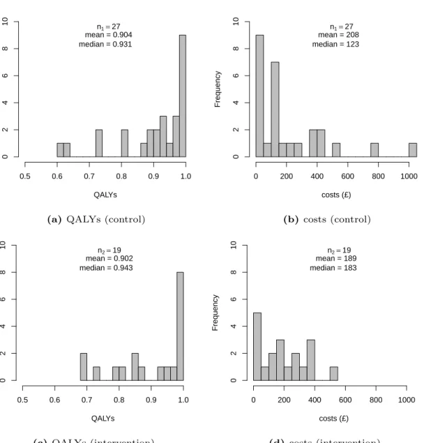
The number of participants completing utility and cost questionnaires at every time point was 27 (36%) and 19 (23%) for the control and intervention group, respectively. Figure 1 shows the histograms of the distributions of the complete case QALYs and costs in the control (panels a-b) and intervention (panels c-d) group, respectively.
FIGURE 1 HERE
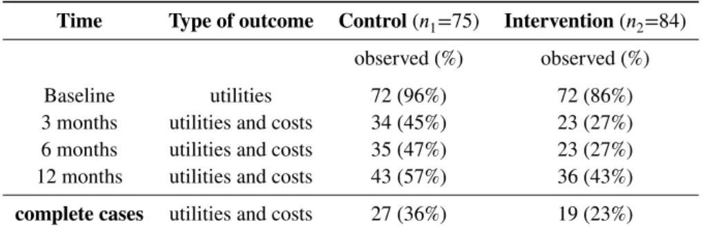
The data clearly present some of the features described in §1. A relatively high degree of skewness characterises the empirical distributions of QALYs and costs in both treatment groups. In particular, the substantial proportion of individuals incurring a perfect health status (which we term “structural ones”) observed in both control (33%) and intervention (42%) groups effectively induces spikes at 1 in the QALYs. Finally, a large proportion of missingness characterises both cost and utility data due to poor follow-up rates. With the exception of baseline data, which are only collected for the utilities, at each time point the two outcomes are either both observed or both missing. A statistical summary of the observed cases and missingness levels for the utility and cost variables by follow up period is shown in Table 1 .
TABLE 1 HERE
The original analysis was performed under a frequentist approach using standard OLS regression.45Baseline utility regression adjustment was incorporated in the model, assuming MAR for all variables and restricting the analysis to the complete cases. However, most of the features described in §1 were not explicitly taken into account.
3
MODELLING FRAMEWORK
In this section, we firstly present our general modelling framework for cost-effectiveness data. The model improves the typical approach used in routine analyses by accounting for correlation between the outcomes. Then it is extended to handle structural values and missing data using three alternative specifications with increasing complexity. Throughout, we refer to our motivating example to demonstrate the flexibility of our full Bayesian approach in dealing with the idiosyncrasies highlighted above; we also note that these are likely to be encountered in many practical cases, thus making our arguments applicable in general.
Assume that some patient-level data are collected from a trial on 𝑖 = 1,…, 𝑛individuals who are randomly allocated to either a control (𝑡 = 1) or intervention (𝑡 = 2) group, with sample sizes𝑛1and𝑛2, respectively. We denote by𝑒𝑖𝑡and𝑐𝑖𝑡the effectiveness and cost outcome variables for the𝑖−th person in group𝑡of the trial. To simplify the notation, unless necessary, we suppress the treatment subscript𝑡.
To account for correlation between the outcomes, in general we can specify the joint distribution𝑝(𝑒, 𝑐)as:
𝑝(𝑒, 𝑐) =𝑝(𝑐)𝑝(𝑒∣𝑐) =𝑝(𝑒)𝑝(𝑐∣𝑒), (2) where, for example,𝑝(𝑒)is themarginaldistribution of the effectiveness and𝑝(𝑐∣𝑒)is theconditionaldistribution of the costs given the effectiveness.15Note that while it is possible to use interchangeably either factorisation in Equation 2, without loss of generality, we describe our analysis in the following through a marginal distribution for the effectiveness (QALYs) and a conditional distribution for the costs.
For each individual we consider a marginal distribution𝑝(𝑒𝑖 ∣ 𝜽𝑒)indexed by a set of parameters𝜽𝑒comprising alocation 𝜙𝑖𝑒and a set ofancillaryparameters𝝍𝑒typically including some measure ofmarginalvariance,𝜎𝑒2. We can model the location parameter using a generalised linear structure, e.g.
𝑔𝑒(𝜙𝑖𝑒) =𝛼0 [+ …],
where𝛼0 is the intercept and the notation[+ …]indicates that other terms (e.g. quantifying the effect of relevant covariates) may or may not be included in the model. In the absence of covariates or assuming that a centered version𝑥∗𝑖 = (𝑥𝑖−̄𝑥)is used, the parameter𝜇𝑒=𝑔𝑒−1(𝛼0)represents the population average effectiveness.
For the costs, we consider a conditional model𝑝(𝑐𝑖∣𝑒𝑖,𝜽𝑐), which explicitly depends on the effectiveness variable, as well as on a set of quantities𝜽𝑐, again comprising a location and ancillary parameters. Note that in this case𝝍𝑐 includes aconditional
variance𝜏𝑐2, which can be typically expressed as a function of the marginal variance𝜎𝑐2.7,15The location can be modelled as a function of the effectiveness variable as:
Here, (𝑒𝑖 −𝜇𝑒) is the centered version of the effectiveness variable, while 𝛽1 quantifies the correlation between costs and effectiveness. Assuming other covariates are either also centered or absent,𝜇𝑐 =𝑔𝑐−1(𝛽0)is the population average cost.
Figure 2 shows a graphical representation of the general modelling framework described above. The effectiveness and cost distributions are represented in terms of combined “modules” — the blue and the red boxes — in which the random quantities are linked through logical relationships. This ensures the full characterisation of the uncertainty for each variable in the model. Notably, this is general enough to be extended to any suitable distributional assumption, as well as to handle covariates in either or both the modules.
FIGURE 2 HERE
In the rest of the section, we present three alternative specifications of the general structure depicted in Figure 2 to model effectiveness and cost data. These are 1) Normal marginal for the effectiveness and Normal conditional for the costs (which is identical to a Bivariate Normal distribution for the two outcomes); 2) Beta marginal for the effectiveness and Gamma conditional for the costs; and 3) Hurdle Model. First, we present each assuming a complete cases scenario and then extend the structure to all cases. The latter scenario includes the complete cases and additionally imputes the outcome values for all the remaining individuals in the trial, either under MAR (for all models) or alternative MNAR scenarios (for the Hurdle Model only).
3.1
Complete Cases
3.1.1
Bivariate Normal
Arguably, the easiest way of jointly modelling two variables is to assume Bivariate normality, which in our context can be factorised into marginal and conditional Normal distributions for𝑒𝑖and𝑐𝑖 ∣𝑒𝑖. This is the closest modelling structure to those underpinning a typical frequentist analysis, while also accounting for potential correlation between the outcomes.
In line with current recommendations (and the original analysis of the MenSS trial), we adjust for the baseline utilities — using a centered version (𝑢𝑖0−̄𝑢0). We model𝑒𝑖∣𝜽𝑒∼Normal(𝜙𝑖𝑒, 𝜎𝑒2), using an identity link function for the location parameter
𝑔𝑒(𝜙𝑖𝑒) =𝜙𝑖𝑒=𝛼0+𝛼1(𝑢𝑖0−̄𝑢0).
Here, the parameter𝛼1quantifies the impact of the centered baseline utilities on the QALYs, while𝜇𝑒=𝛼0and𝜎𝑒2represent the marginal (population level) mean and variance, respectively.
As for the costs, we model𝑐𝑖 ∣𝑒𝑖,𝜽𝑐 ∼Normal(𝜙𝑖𝑐, 𝜏𝑐2), where the conditional mean and variance are defined as
𝑔𝑐(𝜙𝑖𝑐) =𝜙𝑖𝑐=𝛽0+𝛽1(𝑒𝑖−𝜇𝑒) and 𝜏𝑐2=𝜎𝑐2−𝜎𝑒2𝛽12.
The model parameters are thus𝜽𝑒= (𝛼0, 𝛼1, 𝜎2𝑒)and𝜽𝑐= (𝛽0, 𝛽1, 𝜇𝑒, 𝜎2𝑐, 𝜎2𝑒)— note that the marginal mean and variance of the effectiveness link the two modules and therefore feature in both sets of parameters.
The model is completed by assigning suitable prior distributions to the elements of𝜽 = (𝜽𝑒,𝜽𝑐); for example, independent Normal priors can be assumed for the regression parameters, while Uniform or Half-Cauchy priors can be assigned on the scale of the standard deviations.47
3.1.2
Beta-Gamma
The second model we consider assumes a Beta marginal for the QALYs and a Gamma conditional for the costs. In particular, we parameterise the Beta distribution in terms of the mean 𝜙𝑖𝑒 and the scale parameter𝜏𝑖𝑒 = (𝜙𝑖𝑒(1−𝜙𝑖𝑒)
𝜎2
𝑒
− 1)as 𝑒𝑖 ∣ 𝜽𝑒 ∼
Beta(𝜙𝑖𝑒𝜏𝑖𝑒,(1 −𝜙𝑖𝑒)𝜏𝑖𝑒)and model the location as
𝑔𝑒(𝜙𝑖𝑒) =logit(𝜙𝑖𝑒) =𝛼0+𝛼1(𝑢𝑖0−̄𝑢0).
The costs are modelled as𝑐𝑖∣𝑒𝑖,𝜽𝑐 ∼Gamma(𝜙𝑖𝑐𝜏𝑖𝑐, 𝜏𝑖𝑐), where the shape parameter is defined as the product of the location
𝜙𝑖𝑐and the rate𝜏𝑖𝑐. The generalised linear model for the location is
𝑔𝑐(𝜙𝑖𝑐) = log(𝜙𝑖𝑐) =𝛽0+𝛽1(𝑒𝑖−𝜇𝑒).
The marginal means for the QALYs and total costs can then be obtained using the respective inverse link functions
𝜇𝑒=
exp(𝛼0)
Notice that, in comparison to the Bivariate Normal of §3.1.1, the Beta-Gamma model reflects more closely the range and skewness of the observed data. Nevertheless, this modelling structure also fails to directly account for the structural values, e.g. unit QALYs. In the presence of structural values, it is necessary to rescale the observed data, e.g. by applying the Beta model to𝑒∗𝑖 =𝑒𝑖−𝜖for some𝜖→0.
The model is again completed by placing suitable priors on the parameters. For example, we can use independent Normal priors for the regression coefficients(𝛼0, 𝛽0, 𝛼1, 𝛽1)and a Uniform or Half-Cauchy prior for𝜎𝑐. Notice, however, that a little more care is needed in defining a prior distribution for𝜎𝑒. In fact, by the mathematical properties of the Beta distribution, the variance is bounded by a function of the mean
𝜎𝑒2≤𝜇𝑒(1 −𝜇𝑒) =𝜐.
Consequently, we can place an informative prior on the standard deviation𝜎𝑒 ∼ Uniform(0,√𝜐), which coupled with a prior for𝜇𝑒induces a suitable prior for𝜏𝑒as well. Note that even by starting with vague distributions for(𝜇𝑒, 𝜎𝑒), the resulting prior for the Beta scale𝜏𝑒may not be vague at all.
3.1.3
Hurdle Model
To overcome the limitations of the model in §3.1.2 in terms of the structural ones, we expand it to a hurdle version. Specifically, for each subject in the trial𝑖= 1,…, 𝑛we define an indicator variable𝑑𝑖𝑒taking value 1 if the𝑖−th individual is associated with a unit QALYs (𝑒𝑖= 1) and0otherwise (𝑒𝑖<1). This is then modelled as
𝑑𝑖𝑒∶=𝕀(𝑒𝑖= 1) ∼Bernoulli(𝜋𝑖𝑒)
logit(𝜋𝑖𝑒) =𝛾0+𝛾1(𝑢𝑖0− ̄𝑢0) [+ …], (3)
where𝜋𝑖𝑒is the individual probability of unit QALYs, which is estimated on the logit scale as a function of a baseline parameter
𝛾0 and the centred baseline utilities, whose effect is captured by the parameter𝛾1. As for the effectiveness and cost models, other covariates can be additively included in the model of𝑑𝑖𝑒. We specifically distinguish the baseline utilities from any other covariate as they are likely to be particularly informative in predicting whether an individual is associated with a structural one in the QALYs. All the logistic regression parameters should be given suitable prior probability distributions (e.g. Normal). Within this framework, the quantity
̄𝜋𝑒= 1 +exp(𝛾0)
exp(𝛾0) (4)
represents the estimated marginal probability of unit QALYs. The parameters ̄𝜋𝑒and(1 − ̄𝜋𝑒)in effect represent the weights used to mix the two components.
Depending on the value of𝑑𝑖𝑒, we can partition the observed data on the QALYs into two subsets. In the first subset, defined as the𝑛1subjects for whom𝑑𝑖𝑒= 1, we define a variable𝑒𝑖1 = 1. Conversely, the second subset consists of the𝑛<1= (𝑛−𝑛1) subjects for whom𝑑𝑖𝑒= 0and for these individuals we define a variable𝑒<1𝑖 . Because this is less than 1, we can model it directly using a Beta distribution characterised by an overall mean𝜇<1𝑒 , in line with the specification we have shown in §3.1.2. Using the estimated value for ̄𝜋𝑒from Equation 4, we can compute the overall population average effectiveness measure in both treatment groups𝜇𝑒𝑡as the linear combination
𝜇𝑒𝑡= (1 − ̄𝜋𝑒𝑡)𝜇<1𝑒𝑡 + ̄𝜋𝑒𝑡.
In the absence of structural zeros, the conditional model for the costs is exactly as specified in §3.1.2.
3.2
All Cases
When missingness occurs in the QALYs and cost variables, no change to the model structure is required under MAR for both the Bivariate Normal and Beta-Gamma specifications. For the Hurdle Model, when𝑒𝑖 is missing, it is not possible to directly define the value for𝑑𝑖𝑒. However, unit QALYs can only be observed if𝑢𝑖𝑗 = 1for all time points𝑗 = 0,…, 𝐽. Consequently, if an individual𝑖is such that𝑢𝑖𝑗is missing at some time point𝑗and𝑢𝑖𝑗 ≠1at any other time point, then by necessity𝑑𝑖𝑒 = 0. However, for all individuals having𝑢𝑖𝑗 = 1at all observed time points but with at least one missing value at some other time point, then𝑑𝑖𝑒is unknown.
Incomplete covariates need to be explicitly modelled to impute their missing values. For simplicity, we consider the case where the only covariate included in the model is the baseline utility; however, the same approach can be extended to any other type of partially-observed covariates. In the Bivariate Normal and the Beta-Gamma formulations, we can handle missingness in
𝑢𝑖0by assuming a suitable model. One simple choice is to assume the same distribution for𝑢𝑖0as for the outcome𝑒𝑖, i.e. Normal or Beta, respectively — for example, Appendix A shows the implementation for the Beta-Gamma model.
Similarly to §3.1.3, we can formulate another hurdle model for𝑢𝑖0. More specifically, first we specify a model for the indi-viduals with a non-unit utility value. Again, a simple solution is to base this on the same distributions assumed for the QALYs. Secondly, we estimate the probability of observing a structural one in the utilities as
𝑑𝑖𝑢∶=𝕀(𝑢𝑖= 1) ∼Bernoulli(𝜋𝑖𝑢)
logit(𝜋𝑖𝑢) =𝜂0 [+ …] where𝑑𝑖𝑢is the indicator variable for the structural ones in the baseline utilities.
3.2.1
Sensitivity analysis (MNAR)
Finally, Hurdle Models also offer a convenient framework for exploring the robustness of the results to some departures from MAR and therefore allow to perform a simple type of sensitivity analysis to the missingness assumptions. Two relevant cases are:
a) the individuals for whom utility values are missing throughout the follow up, i.e.𝑢𝑖𝑗 =NAfor all𝑗= 1,…, 𝐽;
b) the individuals for whom all the observed utilities are equal to 1, but with at least one time point𝑗at which𝑢𝑖𝑗 =NA. For both these cases, it is impossible to compute the value of the indicator𝑑𝑖𝑒according to the information from the observed data. However, we can arbitrarily set the value of𝑑𝑖𝑒to either 1 or 0 using different configurations, e.g. by varying the number of structural values potentially observed in a given scenario. Since these configurations are based on assumptions about the missing values that cannot be verified from the data at hand (but are in fact arbitrarily set by the experimenter), they effectively represent a way to assess the robustness of the results to some departures from MAR.
In the MenSS trial, there are𝑛∗1 = 13 (12%)individuals in the control and𝑛∗2 = 22 (26%)in the intervention group who fall within caseaorb. Thus, we perform sensitivity analysis by defining a set of alternative MNAR assumption scenarios for these individuals and assess the robustness of the results across them. The four different scenarios considered are summarised in Table 2 :
TABLE 2 HERE
We choose these scenarios in order to assess how different “extreme” combinations of the number of potential structural ones in the intervention and control group can impact the results.
4
RESULTS
We fitted all models usingJAGS,48 a software specifically designed for the analysis of Bayesian models using Markov Chain Monte Carlo (MCMC) simulation, which can be interfaced withRthrough the packageR2jags.49Samples from the posterior distribution of the parameters of interest generated byJAGSand saved to theRworkspace are then used to produce summary statistics and plots. We ran two chains with 20,000 iterations per chain, using a burn-in of 10,000, for a total sample of 20,000 iterations for posterior inference. For each unknown quantity in the model, we assessed convergence and autocorrelation of the MCMC simulations using diagnostic measures such as thepotential scale reduction factorand theeffective sample size.50The total running time required for the models to produce representative samples from the posterior distributions of interest ranged from 5 to 10 minutes.
Alternative prior distributions are considered to check the we are not incorporating any unintended information into the models through the priors. For example, we varied the upper boundary of the uniform distribution and specified alternative prior forms (Half-Cauchy and Half-Normal) for the standard deviations or chose different values for the variance of normally distributed regression parameters. Results were robust to these specifications. Although the Hurdle Model as described in §3.1.3 cannot be directly written inJAGS, it can be implemented using a simple “coding trick”. Appendix A presents all the technical details and theJAGSscript.
4.1
Complete and All Cases (MAR)
Following the original analysis, we first consider only the complete cases and adjust for baseline utilities at the mean level for the QALYs in each model. We initially include in each model three more covariates (age, ethnicity and employment status). However, since posterior results for mean QALYs and costs were almost unaffected by these variables, we simplify the models and retain the covariates only in the linear predictor of Equation 3 to estimate the probability of structural ones in the Hurdle Model. We then extend the framework to all cases under MAR, where the baseline utilities are explicitly modelled as detailed in §3.2 and again as functions of age, ethnicity and employment status. We report the results under MAR as this is the default (and often implicit) missingness assumption used by practitioners in routine analyses. We then conduct a sensitivity analysis to assess the robustness of the results to alternative departures from MAR.
Figure 3 shows the posterior distributions of the mean QALYs and costs for both treatment groups under a complete (red) and all (blue) cases scenario for each model, assuming MAR.
FIGURE 3 HERE
The posterior distributions of the mean QALYs (panels a-b) present some discrepancies between the complete and all cases scenarios, with magnitude varying according to the treatment group and model considered. In general, the results for all cases are lower in the control group and higher in the intervention group in comparison to those obtained using the complete cases. As for the mean costs (panels c-d), the results associated with a Gamma distribution are substantially more skewed compared to those obtaining using the Normal model, especially in the intervention group. In addition, the Gamma model typically leads to mean estimates that are systematically lower under the all cases scenario.
We compare the fit of the different models using the Deviance Information Criterion (DIC).51 The DIC is a measure of comparative predictive ability based on the model deviance and a penalty for model complexity. When comparing a set of models based on the same data, the one associated with the lowest DIC is the best-performing, among those assessed. DIC is not uniquely defined in the presence of missing data and its use and interpretation are not straightforward.52,53No measure of model comparison can provide a full picture of model fit when dealing with partially-observed data. We can compare models based on the fit to the observed data alone, but we must remember that this provides no information about the fit to the unobserved data. In our analysis, we consider a DIC based on the observed data and calculated only for the modules that are in common between the models, i.e. excluding the contribution from the structural indicators for the Hurdle Model. In our analysis, we consider a DIC based on the observed data and calculated only for the modules that are in common between the models, i.e. excluding the contribution from the structural indicators for the Hurdle Model. The Bivariate Normal model is always associated with the highest DIC under both a complete and all cases scenarios (536and445). The Beta-Gamma (386and60) and, especially, the Hurdle model (−50and−2419) substantially improve the model fit to the observed data.
4.1.1
Imputations under MAR
Figure 4 depicts the observed QALYs in both treatment groups (indicated with black crosses) as well as summaries of the posterior distributions for the imputed values, obtained from each model. Imputations are distinguished based on whether the corresponding baseline utility value is observed or missing (blue or red lines and dots, respectively) and are summarised in terms of posterior mean and 90% Highest Posterior Density (HPD) intervals.
FIGURE 4 HERE
There are clear differences in the imputed values and corresponding credible intervals between the three models in both treatment groups. Neither the Bivariate Normal nor the Beta-Gamma models produce imputed values that capture the struc-tural one component in the data. In addition, as to be expected, the Bivariate Normal fails to respect the nastruc-tural support for the observed QALYs, with many of the imputations exceeding the unit threshold bound. These unrealistic imputed values high-light the inadequacy of the Normal distribution for the data and may lead to distorted inferences. Conversely, imputations under the Hurdle Model are more realistic, as they can replicate values in the whole range of the observed data, including the struc-tural ones. Imputed unit QALYs with no discernible interval are only observed in the intervention group due to the original data composition, i.e. individuals associated with a unit baseline utility and missing QALYs are almost exclusively present in the intervention group.
4.2
Sensitivity Analysis (MNAR)
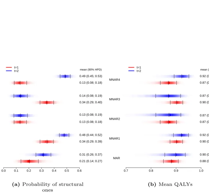
For each of the alternative MNAR scenarios described in §3.2.1, as well as for the analysis under MAR, Figure 5 shows posterior density strips for the structural one probability ̄𝜋𝑒 and the marginal mean QALYs𝜇𝑒, in the control (red) and intervention (blue) groups.
FIGURE 5 HERE
Estimates under MAR indicate that the new intervention is associated with a probability of observing a structural one and a mean QALYs that are on average higher compared to the control. Although similar results are obtained under MNAR1, the estimated quantities are highly unstable across the other three MNAR scenarios. Specifically, under MNAR2 the probability of structural ones is substantially reduced in both groups and induces a zero mean difference in the QALYs. Under MNAR3 and MNAR4 the differences between the estimated probabilities and mean QALYs in the two groups are increased in magnitude and lead to opposite mean differentials.
5
ECONOMIC EVALUATION
We complete the analysis by assessing the cost-effectiveness of the new intervention with respect to the control, comparing the results of the different models under MAR (§ 4.1) and the alternative MNAR scenarios explored for the Hurdle Model (§ 4.2). We specifically rely on the examination of the Cost-Effectiveness Plane (CEP)54and the Cost-Effectiveness Acceptability Curve (CEAC)55to summarise the economic analysis.
FIGURE 6 HERE
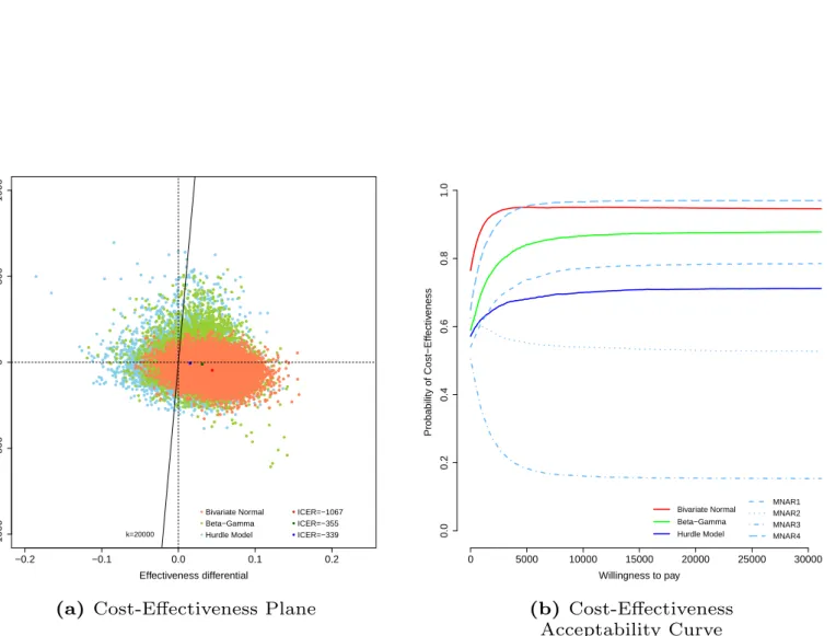
The CEP (Figure 6 , panel a) is a graphical representation of the joint distribution for the population average effectiveness and costs increments, indicated respectively asΔ𝑒= (𝜇𝑒2−𝜇𝑒1)andΔ𝑐= (𝜇𝑐2−𝜇𝑐1), under the three model specifications (light red for the Bivariate Normal, light green for the Beta-Gamma and light blue for the Hurdle Model). The slope of the straight line crossing the plane is the “willingness to pay” threshold (often indicated as𝑘), and can be considered as the amount of budget the decision-maker is willing to spend to increase the health outcome of one unit and effectively is used to trade clinical benefits for money. Points lying below this straight line fall in the so-calledsustainability area7and suggest that the active intervention is more cost-effective than the control. This is because in this area the new intervention is either more effective and less expensive (in the South-Eastern quadrant) or it produces an increase in benefits that more than offsets the increase in the costs (points in the North-Eastern quadrant below the line). In the graph, which for simplicity only displays the results associated with the all cases under MAR, we also show the Incremental Cost-Effectiveness Ratio (ICER) computed under each model, as darker colour dots. This is defined as
ICER= E[Δ𝑐] E[Δ𝑒]
and it quantifies the cost per incremental unit of QALYs. For all three models more than 70% of the samples fall in the sus-tainability area and are associated with negative ICERs, suggesting that the intervention can be considered as cost-effective by producing a QALYs gain at virtually no extra costs, or even saving money.
The CEAC (Figure 6 , panel b) is obtained by computing the proportion of points lying in the sustainability area upon varying the willingness to pay threshold𝑘. Based on general recommended guidelines,1 we consider a range for𝑘up to £30,000 per QALY gained. The CEAC estimates the probability of cost-effectiveness, thus providing a simple summary of the uncertainty associated with the “optimal” decision-making suggested by the ICER. For each model, the results under MAR are reported using solid lines with different colours, i.e. red for the Bivariate Normal, green for the Beta-Gamma and blue for the Hurdle Model. In addition, the results associated with the four MNAR scenarios are reported using different types of dashed lines. Under MAR, for the Bivariate Normal and Beta-Gamma models the CEACs indicate the cost-effectiveness of the new intervention with a probability above0.8for most values of𝑘. Conversely, under the Hurdle Model, the curve is shifted downward by0.24and0.16 with respect to the Bivariate Normal and Beta-Gamma models, respectively, and suggests a more uncertain conclusion. Perhaps unsurprisingly, none of these results is robust to the alternative MNAR scenarios explored. The CEAC plot clearly shows a large sensitivity of the cost-effectiveness probability with respect to the assumed number of structural ones in both treatment groups. Indeed, the curves span a huge probability range from 0.2under MNAR4 to 1under MNAR3. This implies a considerable change in the output of the decision process and severely undermines the validity of the conclusions obtained under MAR.
6
SECOND EXAMPLE: THE PBS TRIAL
The Positive Behaviour Support (PBS)56 trial is a multi-centre RCT involving community intellectual disability services and service users with mild to severe intellectual disability and challenging behaviour. Positive behaviour support is a multicompo-nent intervention which is designed to foster prosocial actions and enhance the person’s quality of life and his/her integration within the local community. Participants (𝑛= 244) were enrolled from a total of𝑆 = 23sites and randomly allocated to staff teams trained to deliver PBS in addition to treatment as usual (reference intervention,𝑛2 = 108), or to staff teams trained to deliver treatment as usual alone (comparator,𝑛1= 136). Measures for quality of life (EQ-5D-3L) and health related cost (family and paid carer records) were collected from each site𝑠at baseline, 6 and 12 months. Utility values lower than zero, representing health states “worse than death”, are recorded for some individuals throughout the study. QALYs and cost variables are computed as in Equation 1. The number of complete cases is 108 (79%) and 96 (89%) for the control and intervention group, respectively. The data in the PBS trial share the same complexities found in the MenSS study. Both QALYs and costs are partially-observed, have skewed empirical distributions and some individuals in both treatment groups are associated with a structural one in the QALYs (5%). The original analysis ignored these features and was performed on the complete cases using standard regression methods, adjusting for differences at baseline utilities and costs, and accounting for the multilevel structure through random effects.
6.1
Models
We show the flexibility of our framework by adapting the models in §3 to accommodate the characteristics of the PBS data. Specifically, we scale the QALYs to avoid negative values when using a Beta distribution, replace the Gamma distribution for the costs with a LogNormal distribution, which improves the fit to the observed data, and account for the multilevel structure.
We assess and compare the performance of three models. These are: 1) Bivariate Normal for the two outcomes; 2) Beta marginal for the effectiveness and LogNormal conditional for the costs; and 3) Hurdle Model. All models account for the multilevel structure in the data and include three categorical covariates (living condition, level of disability and type of carer) to estimate the mean QALYs and costs.
We first apply the models to the complete cases and then extend the analysis to all cases under MAR. No sensitivity analysis as in §3.2.1 can be performed for the PBS study because for each missing individual we observe a utility value that is lower than one at at least one time point, i.e. none of them can be a structural one. In the next section, we present the specification of the Beta-LogNormal model to show how the framework in §3 has been modified to address the characteristics of the PBS data.
6.1.1
Beta-LogNormal
The second model consists of a Beta marginal for the QALYs and a LogNormal conditional for the costs. Since the Beta distri-bution does not allow negative values, we scale the QALYs on(0,1)through the transformation𝑒⋆𝑖 = 𝑒𝑖−min(𝑒𝑖)
max(𝑒𝑖)−min(𝑒𝑖) and fit the model to these transformed variables. A similar scaling is applied to the baseline utilities𝑢⋆𝑖0when these are modelled in the all cases scenario.
The Beta distribution is parameterised as in §3.1.2, while the multilevel structure is accounted for through site-specific regres-sion coefficients for the baseline utility and cost terms (varying-slope only model). We choose this specification as inference from a varying-intercept model was similar to that obtained from ignoring the multilevel structure, while the introduction of site-specific coefficients for the other covariate terms lead to almost identical results compared with the proposed approach.
The QALYs are modelled as𝑒⋆𝑖 ∣𝜽𝑒∼Beta(𝜙𝑖𝑒𝜏𝑖𝑒,(1 −𝜙𝑖𝑒)𝜏𝑖𝑒)with location logit(𝜙𝑖𝑒) =𝛼0+𝛼1𝑠(𝑢𝑖0− ̄𝑢0) [+ …]
where𝛼1𝑠are the baseline utility structured coefficients associated with the𝑠= 1,…, 𝑆different sites.
The costs are modelled as𝑐𝑖∣𝑒⋆𝑖,𝜽𝑐 ∼LogNormal(𝜙𝑖𝑐, 𝜏𝑐), where the mean and standard deviation parameters(𝜙𝑖𝑐, 𝜏𝑐)are defined on the log scale. Baseline costs(𝑐0)are included in the cost model using the same multilevel specification used for𝑢0 in the QALYs model. It is not possible to include the centered QALYs in the regression as modelling𝑒⋆𝑖 on a transformed scale does not allow to identify the marginal mean𝜇𝑒as in §3.1.2. Consequently, the cost location is
𝜙𝑖𝑐=𝛽0+𝛽1(𝑒⋆𝑖) +𝛽2𝑠(𝑐𝑖0− ̄𝑐0) [+ …]
We retrieve the marginal means on the natural scale for both outcomes through Monte Carlo integration. At each iteration of the posterior distribution for the model parameters in the MCMC output, we generate a large number of samples for𝑒𝑖 and𝑐𝑖 and take the expectation over these values to obtain Monte Carlo estimates of the marginal means𝜇𝑒and𝜇𝑐.
To complete the model we specify Normal priors for the structured coefficients𝛼1𝑠∼Normal(0, 𝜎𝛼)and𝛽2𝑠∼Normal(0, 𝜎𝛽) with shared standard deviations𝜎𝛼and𝜎𝛽. Finally, we choose independent Normal priors for the other regression coefficients
𝜶and𝜷and a Uniform or Half-Cauchy prior for the standard deviations.
6.2
Results
All models are fitted and assessed using the same software configuration and diagnostic measures as in §4. Due to space constraints, we only present the economic results for each model in the PBS study for the all cases scenario under MAR. A comparison of the posterior inference between the models for both the complete and all cases scenarios, the imputed QALYs for each model under MAR and a summary and visual description of the PBS data are available on the Web Appendix.
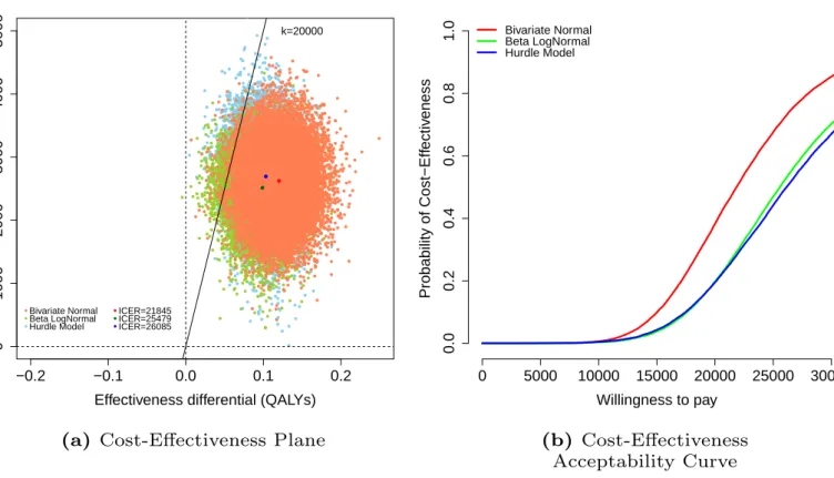
Figure 7 shows the CEP and CEAC for the Bivariate Normal (red dots and line), Beta-LogNormal (green dots and line) and Hurdle Model (blue dots and line) for the all cases scenario under MAR.
FIGURE 7 HERE
For all three models, almost all samples in the CEPs (Figure 7 , panel a) are located in the North-Eastern quadrant and most of them fall in the sustainability area at a willingness to pay𝑘=£20,000. Results from the Bivariate Normal model suggests a higher cost-effectiveness of the new intervention and are associated with a lower ICER compared with those of the other two models. This is reflected in the CEACs (Figure 7 , panel b) which show a probability of cost-effectiveness that is on average 20%higher for the Bivariate Normal with respect to the Beta-LogNormal and Hurdle Model.
7
DISCUSSION
In CEAs alongside RCTs, analysts typically rely on standard models that ignore or at best fail to properly account for poten-tially important features in the data, such as the correlation between costs and effectiveness, skewness in the distribution of the observed data, the presence of structural values and, almost invariably, missing data. In this paper, we have presented a gen-eral Bayesian framework that is able to overcome these problems. Our approach represents a considerable improvement with respect to the current practice and can be implemented in a relatively easy way using freely available software. This is a key advantage that can encourage practitioners to move away from likely biased methods and promote the use of our framework in routine analyses.
The analysis of both case studies shows notable variations in the results, compared with those of the original analyses. In the MenSS trial, accounting for the structural ones and missingness uncertainty has a considerable impact on the cost-effectiveness of the new intervention and future research prioritisation. In particular, the sensitivity of the final conclusions to the missingness scenarios suggests that the results obtained under MAR are not robust to the departures explored. This is expected in light of the large proportion of missing values and the limited auxiliary information available. The original analysis ignored missingness uncertainty and therefore its conclusions are unlikely to provide a reliable picture about the economic assessment. Our analysis of the MenSS trial illustrates how a model that accounts for the complexities of the data can be specified using our framework and shows the difficulty of drawing any conclusion from this study given the limited evidence available and the lack of robustness of the results to the missing data assumptions. In the PBS trial, the results of the economic evaluation change substantially when skewness is accounted for. This second example demonstrates the flexibility of our framework and compares alternative model specifications in a setting where the data have a multilevel structure and the proportion of missing values is lower with respect to the MenSS trial. In both cases, the Hurdle Model represents the best model among those assessed as it captures both skewness and structural values, while the other specifications fail to deal with at least one of these features.
Our results are obtained with specific reference to the two case studies. However, the MenSS and PBS trials are very much rep-resentative of the “typical” dataset used in CEAs alongside RCTs. Thus, it is highly likely that the same features (and potentially the same contradictions in the results, upon varying the complexity of the modelling assumptions) apply to many real cases. This is a very important, if somewhat overlooked problem, as it can thwart the validity of simplistic models that, while established among practitioners, may lead to misleading cost-effectiveness conclusions and bias the decision-making process.
Missing data pose a serious threat to the economic evaluation as, when confronted with a partially-observed dataset, each analysis makes assumptions about the missing values that cannot be verified from the data at hand. Any measure of fit or predictive accuracy, such as the DIC or Posterior Predictive Checks,50 can only provide information about the observed data and therefore tell just part of the story.52,53Thus, the use of sensitivity analysis to explore the impact on the results of different plausible missingness assumptions, including MNAR, becomes essential. The Bayesian approach naturally allows to perform these assessments through the incorporation of external evidence (e.g. expert opinions) in the model using prior distributions while ensuring consistency and the correct propagation of uncertainty throughout the model.
We have demonstrated one possible way of assessing the robustness of the results to some “extreme” scenarios that can be incorporated in the framework at no extra cost in terms of model complexity. If the results are not robust to the departures explored, these scenarios offer a starting point for further analyses where more advanced methods can be used to explicitly allow for the variability in the MNAR values, e.g. Selection Models or Pattern Mixture Models.42,43,44Practitioners could incorporate strategies at the design stage of the trial to collect data from external sources, which can be used to guide the missingness assumptions in the statistical analysis. For example, additional information can be obtained through the elicitation of experts’ knowledge or the inclusion of auxiliary variables that are thought to be predictive of missingness.
Finally, a potentially relevant question concerning missing variables derived from repeated questionnaires, e.g. EQ-5D, is whether imputation should be carried out at the time scores (utilities) or total scores (QALYs) level. The performance of these alternative imputation strategies has only recently been compared in the health economic literature.57,58,59The cross-sectional modelling framework used in trial-based economic evaluations has some limitations for handling missingness because it does not allow for the incorporation of the information from the partially-observed utilities and costs in the study or the time depen-dence between the responses. These limitations can be overcome using a modelling framework that explicitly accounts for the longitudinal nature of the data. In future work we plan to develop a longitudinal model to efficiently deal with missingness while also jointly accounting for the complexities of the data in economic evaluations. This, however, requires a radical change of the model paradigm currently used by practitioners and a level of statistical knowledge that would undermine the ease of implementation of our framework in routine analyses and therefore goes beyond the objective of this paper.
In conclusion, in this work we have presented a flexible Bayesian analytic framework that can:a)jointly model costs and effectiveness;b)account for skewness and structural values; andc)assess the robustness of the results under a set of differing missingness assumptions. Routine analyses almost exclusively rely on methods that ignore at least some of the complexities of the data. The original contribution of this work consists in the joint implementation of methods that account for these complexities within a unique and flexible framework that is relatively easy to apply. It is important that the features of CEA individual-level data are simultaneously addressed to avoid biased results, which may in turn lead to misleading cost-effectiveness conclusions. The availability of methodological and practical tools such as the ones presented in this paper have the potential to improve the work of modellers and regulators alike, thus advancing the fields of economic evaluation of health care interventions.
ACKNOWLEDGEMENT
Mr Andrea Gabrio is partially funded in his PhD programme at University College London by a research grant sponsored by The Foundation BLANCEFLOR Boncompagni Ludovisi, née Bildt.
Dr Gianluca Baio is partially supported as the recipient of an unrestricted research grant sponsored by Mapi Group at University College London.
Finally, we wish to thank Ms Julia V. Bailey, Ms Angela Hassiotis and Ms Rachael Hunter at University College London for providing the MenSS and PBS trial data and advise on the original economic model.
References
1. NICE .Guide to the Methods of Technological Appraisal. London, UK: NICE; 2013.
2. Briggs A. Handling uncertainty in cost-effectiveness models.Pharmaco Economics.2000;22:479-500.
3. OHagan A, McCabe C, Hakehurst R, et al. Incorporation of uncertainty in health economic modelling studies.Pharmaco Economics.2004;23:529-536.
4. Sculpher M, Claxton K, Drummond M, McCabe C. Whither trial-based economic evaluation for health decision making?.
Health Economics.2005;15:677-687.
5. Spiegelhalter D, Best N. Bayesian approaches to multiple sources of evidence and uncertainty in complex cost-effectiveness modelling.Statistics in Medicine.2003;22:3687-3709.
6. Claxton K. The irrelevance of inference: a decision making approach to stochastic evaluation of health care technologies.
Journal of Health Economics.1999;18:342-364.
7. Baio G.Bayesian Methods in Health Economics. University College London, London, UK: Chapman and Hall/CRC; 2012. 8. Jackson C, Thompson S, Sharples L. Accounting for uncertainty in health economic decision models by using model
averaging.Journal of the Royal Statistical Society: Series A.2009;172:383-404.
9. Briggs A, Schulpher M, Claxton K.Decision Modelling for Health Economic Evaluation. Oxford, UK: Oxford university press; 2006.
10. Spiegelhalter DJ, Abrams KR, Myles JP.Bayesian approaches to clinical trials and health-care evaluation. John Wiley and Sons; 2004.
11. Manca A, Hawkins N, Sculpher MJ. Estimating mean QALYs in trial-based cost-effectiveness analysis: the importance of controlling for baseline utility.Health Economics.2005;14:487-496.
12. Hunter RM, Baio G, Butt T, Morris S, Round J, Freemantle N. An Educational Review of the Statistical Issues in Analysing Utility Data for Cost-Utility Analysis.Pharmaco Economics.2015;33:355-366.
13. European Medicines Agency . Committee for Medicinal Products for Human Use (CHMP). Guideline on adjust-ment for baseline covariates. http://www.ema.europa.eu/docs/en_GB/document_library/Scientific_guideline/2013/06/ WC500144946.pdf; 2013.
14. O’Hagan A, Stevens JW. A Framework for Cost-Effectiveness Analysis from Clinical Trial Data. Health Economics.
2001;10:303-315.
15. Nixon RM, Thompson SG. Methods for incorporating covariate adjustment, subgroup analysis and between-centre differences into cost-effectiveness evaluations.Health Economics.2005;14:1217-1229.
16. Thompson SG, Nixon RM. How Sensitive Are Cost-Effectiveness Analyses to Choice of Parametric Distributions?.Medical Decision Making.2005;4:416-423.
17. Briggs A, Gray A. The distribution of health care costs and their statistical analysis for economic evaluation.Health Serv Res Pol.1998;3:233-245.
18. Rascati KL, Smith LJ, Neilands T. Dealing with Skewed Data: An Example Using Asthma-Related Costs of Medicaid Clients.Health Economics.2001;23:481-498.
19. O’Hagan A, Stevens JW. Assessing and comparing costs: how robust are the bootstrap and methods based on asymptotic normality?Health Economics.2003;12:33-49.
20. Basu A, Manca A. Regression Estimators for Generic Health-Related Quality of Life and Quality-Adjusted Life Years.
Medical Decision Making.2012;1:56-69.
21. Cooper N, Sutton AJ, Mugford M, Abrams K. Use of Bayesian Markov Chain Monte Carlo Methods to Model Cost-of-Illness Data.Medical Decision Making.2003;23:38-53.
22. Mihaylova B, Briggs A, O’Hagan A, Thompson SG. Review of Statistical Methods for Analysing Healthcare Resources and Costs.Health Economics.2011;20:897-916.
24. Baio G. Bayesian models for cost-effectiveness analysis in the presence of structural zero costs. Statistics in Medicine.
2014;33:1900-1913.
25. Tooze J, Grunwald G, Jones K. Analysis of repeated measures data with clumping at zero.Statistical Methods in Medical Research.2002;211:341-355.
26. Harkanen T, Maljanen T, Lindfors O, Virtala E, Knekt P. Confounding and Missing Data in Cost-Effectiveness Analysis: Comparing different methods.Health Economics Review.2013;28:3-8.
27. Ramsey SD, Willke RJ, Glick H, et al. Cost-Effectiveness Analysis Alongside Clinical Trials II-An ISPOR Good Research Practices Task Force Report.Value in Health.2015;18:161-172.
28. Groenwold RHH, Rogier A, Donders T, Roes KCB, Harrell FE, Moons KGM. Dealing With Missing Outcome Data in Randomized Trials and Observational Studies.American Journal of Epidemiology.2012;175:210-217.
29. Wood AM, White IR, Thompson SG. Are missing outcome data adequately handled?A review of published randomized controlled trials in major medical journals.Clinical Trials.2004;1:368-376.
30. Noble SM, Hollingworth W, Tilling K. Missing data in trial-based cost-effectiveness analysis: the current state of play.
Health Economics.2012;21:187-200.
31. Gabrio A, Mason AJ, Baio G. Handling Missing Data in Within-Trial Cost-Effectiveness Analysis: A Review with Future Recommendations.Pharmaco Economics-Open.2017;1:79-97.
32. Briggs A, Clark T, Wolstenholme J, Clarke P. Missing. . . . presumed at random: cost-analysis of incomplete data.Health Economics.2003;12:377-392.
33. Manca P, Palmer S. Handling Missing Data in Patient-Level Cost-Effectiveness Analysis Alongside Randomised Clinical Trials.Appl Health Econ Health Policy.2005;4:65-75.
34. Faria R, Gomes M, Epstein D, White IR. A Guide to Handling Missing Data in Cost-Effectiveness Analysis Conducted Within Randomised Controlled Trials.Pharmaco Economics.2014;32:1157-1170.
35. Rubin DB.Multiple Imputation for Nonresponse in Surveys. New York, US: John Wiley and Sons; 1987.
36. Diaz-Ordaz K, Kenward MG, Grieve R. Handling missing values in cost effectiveness analyses that use data from cluster randomized trials.Journal of the Royal Statistical Society: Series A.2014;177:457-474.
37. Burton A, Billingham LJ, Bryan S. Cost-effectiveness in clinical trials: using multiple imputation to deal with incomplete cost data.Clinical Trials.2007;4:154-161.
38. Schafer JL.Analysis of Incomplete Multivariate Data. New York, US: Chapman and Hall; 1997.
39. Schafer JL. Multiple imputation for multivariate missing data problems: A data analyst’s perspective. Multivariate Behavioural Research.1998;33:545-571.
40. Van Buuren S, Groothuis-Oudshoorn K. mice: Multivariate Imputation by Chained Equations in R.Journal of Statistical Software.2011;45:1-67.
41. Carpenter JR, Kenward MG, IR White. Sensitivity analysis after multiple imputation under missing at random: a weighting approach.Statistical Methods in Medical Research.2007;16:259-275.
42. Molenberghs G, Fitzmaurice G, Kenward MG, Tsiatis A, Verbeke G.Handbook of Missing Data Methodology. Boca Raton, FL: Chapman and Hall; 2015.
43. Daniels MJ, Hogan JW.Missing Data in Longitudinal Studies: Strategies for Bayesian Modeling and Sensitivity Analysis. New York, US: Chapman and Hall; 2008.
44. Mason A, Richardson S, Plewis I, Best N. Strategy for Modelling Nonrandom Missing Data Mechanisms in Observational Studies Using Bayesian Methods.Journal of Official Statistics.2012;28:279-302.
45. Bailey JV, Webster R, Hunter R, et al. The Mens’s Safer Sex project: intervention development and feasibility randomised controlled trial of an interactive digital intervention to increase condom use in men.Health Technology Assessment.2016;20. 46. Drummond MF, Schulpher MJ, Claxton K, Stoddart GL, Torrance GW.Methods for the economic evaluation of health care
programmes. 3rd ed. Oxford, UK: Oxford University Press; 2005.
47. Gelman A. Prior distributions for variance parameters in hierarchical models.Bayesian Analysis.2006;1:515-533. 48. Plummer M.JAGS: Just Another Gibbs Sampler. http://www-fis.iarc.fr/~martyn/software/jags/; 2010.
49. Su YS, Yajima M.Package ‘R2jags’. http://www-fis.iarc.fr/~martyn/software/jags/; 2015.
50. Gelman A, Carlin J, Stern H, Rubin D.Bayesian Data Analysis - 2nd edition. New York, NY: Chapman and Hall; 2004. 51. Spiegelhalter DJ, Best NG, Carlin BP, Linde A. Bayesian measures of model complexity and fit. Journal of the Royal
Statistical Society.2002;64:583-639.
52. Celeux G, Forbes S, Robert CP, Titterington DM. Deviance Information Criteria for Missing Data Models. Bayesian Analysis.2006;1:651-674.
53. Mason A, Richardson S, Best N. Two-pronged Strategy for Using DIC to Compare Selection Models with Non-Ignorable Missing Responses.Bayesian Analysis.2012;7:109-146.
54. Black WC. A Graphic Representation of Cost-Effectiveness.Medical Decision Making.1990;10:212-214.
55. Van Hout BA, Al MJ, Gordon GS, Rutten FFH, Kuntz KM. Costs, Effects and C/E-Ratios Alongside a Clinical Trial.Health Economics.1994;3:309-319.
56. Hassiotis A, Poppe M, Strydom A, et al. Positive behaviour support training for staff for treating challenging behaviour in people with intellectual disabilities: a cluster RCT.Health Technology Assessment.2018;22.
57. Lambert PC, Billingham LJ, Cooper NJ, Sutton AJ, Abrams KR. Estimating the cost-effectiveness of an intervention in a clinical trial when partial cost information is available: a Bayesian approach.Health Economics.2008;17:67-81.
58. Eekhout I.Don’t Miss Out!: Incomplete data can contain valuable information. Amsterdam, NL: EMGO+ Institute for Health and Care Research, Department of Epidemiology and Biostatistics, VU University Medical Center; 2014.
59. Simons CL, Rivero-Arias O, Yu LM, Simon J. Multiple imputation to deal with missing EQ-5D-3L data: Should we impute individual domains or the actual index?.Qual Life Res.2015;24:805-815.