Clemson University
TigerPrints
All Dissertations Dissertations
8-2013
Mobile Robot Navigation for Person Following in
Indoor Environments
Ninad Pradhan
Clemson University, [email protected]
Follow this and additional works at:https://tigerprints.clemson.edu/all_dissertations Part of theRobotics Commons
This Dissertation is brought to you for free and open access by the Dissertations at TigerPrints. It has been accepted for inclusion in All Dissertations by an authorized administrator of TigerPrints. For more information, please [email protected].
Recommended Citation
Pradhan, Ninad, "Mobile Robot Navigation for Person Following in Indoor Environments" (2013).All Dissertations. 1186.
Mobile Robot Navigation for Person Following
in Indoor Environments
A Dissertation Presented to the Graduate School of
Clemson University
In Partial Fulfillment
of the Requirements for the Degree Doctor of Philosophy Computer Engineering by Ninad Pradhan August 2013 Accepted by:
Dr. Timothy Burg, Committee Chair Dr. Stan Birchfield (co-advisor)
Dr. Ian Walker Dr. Damon Woodard
Abstract
Service robotics is a rapidly growing area of interest in robotics research. Ser-vice robots inhabit human-populated environments and carry out specific tasks. The goal of this dissertation is to develop a service robot capable of following a human leader around populated indoor environments. A classification system for person followers is proposed such that it clearly defines the expected interaction between the leader and the robotic follower. In populated environments, the robot needs to be able to detect and identify its leader and track the leader through occlusions, a common characteristic of populated spaces. An appearance-based person descriptor, which augments the Kinect skeletal tracker, is developed and its performance in de-tecting and overcoming short and long-term leader occlusions is demonstrated. While following its leader, the robot has to ensure that it does not collide with stationary and moving obstacles, including other humans, in the environment. This requirement necessitates the use of a systematic navigation algorithm. A modified version of navi-gation function path planning, called the predictive fields path planner, is developed. This path planner models the motion of obstacles, uses a simplified representation of practical workspaces, and generates bounded, stable control inputs which guide the robot to its desired position without collisions with obstacles. The predictive fields path planner is experimentally verified on a non-person follower system and then integrated into the robot navigation module of the person follower system. To
navigate the robot, it is necessary to localize it within its environment. A mapping approach based on depth data from the Kinect RGB-D sensor is used in generating a local map of the environment. The map is generated by combining inter-frame rotation and translation estimates based on scan generation and dead reckoning re-spectively. Thus, a complete mobile robot navigation system for person following in indoor environments is presented.
Dedication
To my parents, for their love and sacrifice.
To my sister Meeta, for her altruism and compassion.
To Kaveri, without whom it would be impossible to see any part of this become reality.
Acknowledgments
My advisors, Dr. Burg and Dr. Birchfield, were kind enough to accept mentor-ing me durmentor-ing my Ph.D., and I thank them for helpmentor-ing me understand the complexity of research. There were times where I was myopic about my own research and, looking back, I realize how incomplete this dissertation would be without their encouragement to never lose sight of the bigger picture.
Dr. Walker and Dr. Woodard were always available for advice and feedback, and the points they raised during my proposal presentation went a long way towards providing corrective inputs for the final outcome. During my collaboration with Dr. Neeraj Gohad, I benefited from his insights and his passion and excitement for research.
Lane Passalacqua Swanson went out of her way to help me when I had to face the perfect storm of qualifier preparations and medical issues. Having people like her and Elizabeth Gibisch in the department staff has made life easier for me and countless other graduate students. I also thank David Moline and John Hicks for their help on many occasions.
The example of dedication and diligence set by my friends and roommates Nihar Ranjan and Sunil Kumar will stay with me for a long time. We share a love for long discussions and for endless debates. Their humor and congeniality were vital to a great friendship.
From nearly the beginning of my Clemson years, Ravi Joseph Singapogu has been a steadfast friend and a wonderful source of encouragement. He, his wife Rachel, and his children David, Asha, and Priya, have been my window into life beyond the lab in our college town.
Any mention of my Clemson years would be incomplete without of those who I have been lucky to know since the very beginning: Utpal, Ujwal, Lalit, Neha, Radhika, Swapna, Sushant.
Without my colleagues and friends Apoorva Kapadia, Tony Threatt, Jessica Merino, and Bryan Willimon, these past few years would be much less fun.
My research benefited from collaborating or discussing ideas with Brian Peasley and Sean Ficht. Vikram Iyengar, Sumod Mohan, Vidya Gayash, and Nitendra Nath were exemplary in their aptitude and love for research and problem solving.
Rahul Saxena, Raghvendra Cowlagi, and Salil Wadhavkar constantly amaze me with their proficiency and deep insights on diverse topics. They, along with Chetan Danait, Rohit Pradhan, Ananya Sanyal, Abhijeet Malik, and Rajula Subramanian, were a vital part of my undergraduate years and remain close to me still.
In Shripad Kulkarni, Bankim Ghelani, and Aditi Nerikar, I have been lucky to have friends who have been a solid and constant influence in my life for many years. My family has always shown me the way, and my strengths, such as they might be, can be attributed to the example of my parents, sister, aunt, and grandparents.
Finally, I have been fortunate to have the permanent presence and support of Kaveri, Shamila Thakur-Bhatia, Gautam Bhatia, and Dinesh Thakur through these years.
Table of Contents
Title Page . . . i Abstract . . . ii Dedication . . . iv Acknowledgments . . . v List of Tables . . . ix List of Figures . . . x 1 Introduction . . . 11.1 Service robots in recent literature . . . 1
1.2 Person followers . . . 3
1.3 Dissertation outline . . . 16
2 Development of predictive fields path planning . . . 17
2.1 Navigation function path planning. . . 18
2.2 Development of an elliptical repulsion function . . . 27
2.3 Development of directional control input . . . 45
2.4 Development of workspace generation method . . . 48
3 Experimental verification of predictive fields path planning . . . . 57
3.1 Outline of the experiment . . . 58
3.2 Controlling the robot . . . 61
3.3 Workspace and wall obstacle representation . . . 63
3.4 Robot and internal obstacle tracking . . . 69
3.5 Results . . . 77
4 Person following in indoor environments . . . 92
4.1 A classification system for person following . . . 93
4.2 Leader tracking using color descriptors . . . 103
4.4 Person following using predictive fields . . . 141
5 Conclusions and future work . . . 151
5.1 Conclusions . . . 151
5.2 Future work . . . 154
List of Tables
List of Figures
1.1 Block diagram of the person follower system. . . 4
2.1 Bump function used for workspace envelope repulsion.. . . 22
2.2 Path to goal using standard navigation functions. . . 24
2.3 High velocity inputs to robot. . . 25
2.4 Transformation from a star world to a circular world. . . 26
2.5 Transition from circular to elliptical field. . . 28
2.6 A sample robot approach to obstacle ellipse. . . 31
2.7 Repulsion term v. robot distance from obstacle ellipse. . . 32
2.8 The path of the robot without predictive information. . . 36
2.9 The path of the robot with predictive information.. . . 37
2.10 The path of the robot without predictive information. . . 39
2.11 The path of the robot with predictive information.. . . 40
2.12 Route in absence and presence of predictive fields. . . 41
2.13 Calculation basis for the risk score. . . 42
2.14 Individual components of the unit velocity vector. . . 45
2.15 Generation of workspace compatible with navigation functions. . . 49
2.16 Generation of leader waypoints as the robot follows the leader. . . 51
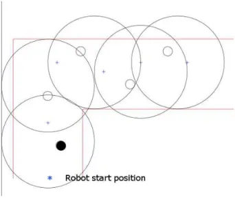
2.17 Multiple workspaces with predictive fields. . . 53
2.18 Multiple workspaces without predictive fields. . . 54
2.19 Multiple workspaces with stationary obstacles. . . 55
3.1 Procedure for predictive path planning experiment. . . 58
3.2 Schematic of Roomba remote control interface . . . 62
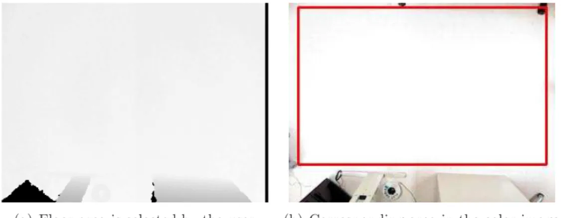
3.3 Selection of points for estimation of floor plane equation. . . 64
3.4 Labeling wall obstacle lines. . . 66
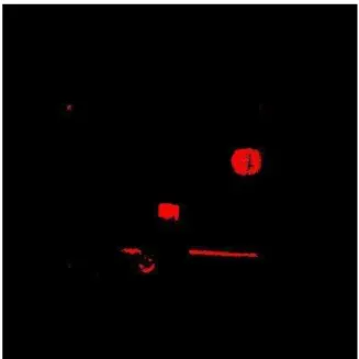
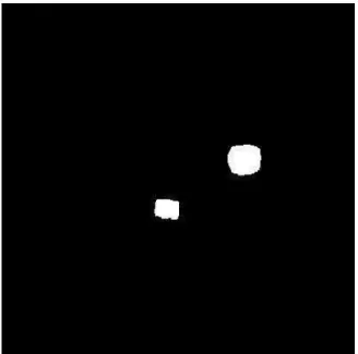
3.5 Occupancy map generated after floor segmentation . . . 67
3.6 Morphological processing of occupancy image . . . 68
3.7 Initialization of the internal object tracker . . . 70
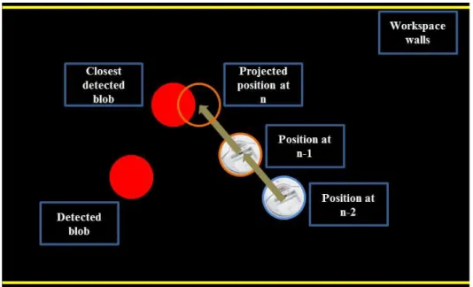
3.8 Prediction of object position and matching to detected blob . . . 71
3.9 Calibration of hue and saturation values to identify markers . . . 72
3.10 Output of heading estimation . . . 73
3.11 Generation of obstacle ellipse . . . 75
3.13 Convergence to goal with a single stationary obstacle . . . 81
3.14 Convergence to goal with a two stationary obstacles . . . 82
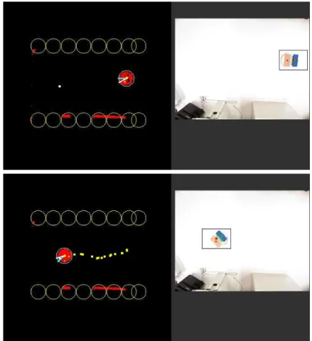
3.15 Example 1 of convergence to goal with moving obstacle, no ellipse. . . 84
3.16 Example 1 of convergence to goal with moving obstacle with ellipse. . 85
3.17 Example 1 with ellipse generated around obstacle. . . 86
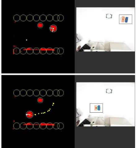
3.18 Example 1: Comparing robot positions with and without use of ellipse 88 3.19 Example 2 of convergence to goal with moving obstacle, no ellipse. . . 89
3.20 Example 2 of convergence to goal with moving obstacle with ellipse. . 90
3.21 Example 2 with ellipse generated around obstacle. . . 91
4.1 Level 1 person follower . . . 95
4.2 Level 2 person follower . . . 97
4.3 Level 3 person follower . . . 99
4.4 Level 4 person follower . . . 101
4.5 Skeletal representation in the Kinect SDK . . . 104
4.6 Skeletal outline overlaid on RGB image . . . 105
4.7 Bone patch extracted from the skeletal outline.. . . 108
4.8 Example of self-occlusion . . . 110
4.9 Using bone angles to infer self-occlusion. . . 111
4.10 Comparison of descriptors from same trial . . . 113
4.11 Comparison of descriptors from different trials . . . 114
4.12 Tabulated results from leader-non leader comparisons . . . 115
4.13 Leader tracking before occlusion. . . 116
4.14 Detected occlusion. . . 117
4.15 Leader recovery after occusion. . . 118
4.16 Typical hallways for person following. . . 120
4.17 Poor results from feature tracking. . . 121
4.18 Poor results from scan matching. . . 123
4.19 Generation of occupancy map from Kinect data . . . 124
4.20 Generation of polar scans from occupancy maps . . . 125
4.21 Multi-line RANSAC estimates from scan data . . . 127
4.22 Reference bins for Manhattan estimate. . . 132
4.23 Sample mapping frame for Manhattan estimate. . . 134
4.24 Map output down a straight hallway. . . 137
4.25 Map output at a L-junction. . . 138
4.26 Map output at a T-junction. . . 140
4.27 Initialization for a trial.. . . 142
4.28 Transition from exact following to path planning. . . 144
4.29 Path planning to overcome sensor range occlusion. . . 146
4.30 Path planning around a single stationary person. . . 148
4.31 Path planning around a moving occluding person. . . 149
Chapter 1
Introduction
As robots make a gradual transition from industrial settings to household or personal applications, direct interaction between humans and robots has become an emerging area of research. In this dissertation, a person following mobile robotic system is developed and its results presented.
Person followers are part of the larger robot classification called ‘service robots’
[1]. Service robots are robots which operate in human populated environments and
assist people in their daily activities. This is a broad definition which is satisfied by a growing number of robotics systems described in recent literature.
1.1
Service robots in recent literature
‘Grace’, developed in 2007 by Kirby et al. [2], was designed to accompany a
person around using verbal and non-verbal cues for interaction. Scans from a laser range finder were used to infer the presence and location of a person, with whom the robot communicated using vocalization. The leader was informed by the robot when a change of state, such as the leader stopping or moving out of robot sensor range,
was detected. ‘Minerva’, developed in 2000 by Thrun et al. [3], was designed to act as a tour guide. The robot localized itself relative to a map of its test environment, the Smithsonian Museum of American History. The robot avoided collisions with visitors
and executed multiple tours of the museum as a guide. Its predecessor, ‘Rhino’ [4],
developed in 1995 by Buhmann et al., achieved similar objectives of mapping and avoiding collisions in an indoor environment. ‘BIRON’, developed in 2004 by Haasch et al. [5], is another well known service robot which was designed to actively interact with its user by means of speech and gesture recognition. ‘MKR’, developed in 2010 by Takahashi et al. [6], is a hospital service robot which transports luggage, specimens, etc. around hospital passages using potential fields for navigation.
Some recent service robotics systems are close to, or already in the process of, commercial production and distribution. Probably the best known of these is the ‘Care-o-botR
3’, developed in 2009 by Reiser et al. [7]. This robot is equipped with
laser range scanners, a vision system, and a 7-DOF (Degrees-of-freedom) manipulator arm. One typical application of this robot is to serve as a robotic butler. For example, a customer may ask for a drink using a touchscreen on the robot. The robot then identifies the requested object in the inventory of bottles or cans using an object recognition module, and the grasping mechanism then lifts the correct object and the robot returns to the customer to serve it. This robot is a typical example of integrating various modules to create a useful robotic system. ‘Johnny’, developed in 2012 by Breuer et al. [8], can be considered to be another state-of-the-art service
robot. Based on the requirements of the RoboCup@Home challenge [9], this robot was
designed to serve in a restaurant-like environment, where it received seat reservations, waited on guests, and delivered orders to them.
Providing service and care in domestic environments is a fairly prevalent theme
service robot designed to interact with people with mild dementia. It was equipped with telepresence software, which would allow remote medical consultation, and with a speech recognition system which would allow the user to communicate with the robot. The robot navigated around an indoor environment by first creating a map using learning techniques and then being able to move to an arbitrary location using
this map. ‘CompanionAble’, developed in 2011 by Gross et al. [11], was designed to
assist the elderly who suffer from mild cognitive impairment, in home environments. This project was geared towards developing home robots with telepresence and with the capability to detect hazardous events such as falls and using telepresence to allow the patient to communicate with caregivers. With a growing fraction of the elderly living alone in the US [12], such robots are placed to fill a void in the care afforded
to this section of the population. ‘Hein II’, developed in 2011 by Tani et al. [13],
was designed as a person follower for home oxygen therapy patients. Such patients need to tether around an oxygen supplier tank, which can be physically exhausting. A large number of people in Japan, where this robot was designed, are dependent on
home oxygen therapy [14], and such a robotic follower would provide an improvement
to their quality of life. Thus service robots, or ‘socially assistive robots’, as they have also been called [15], are gradually maturing into a useful technology.
1.2
Person followers
The development of the person following mobile robot system described here was characterized by the same desire to realize a robot capable of interacting with humans in an everyday environment.
An environment populated with humans poses multiple challenges to a robot which seeks to follow a leader within it:
Figure 1.1: Block diagram of the person follower system.
• Detecting and tracking the leader.
• Detecting and handling leader occlusion.
• Avoiding collisions with walls, people, and objects.
• Identifying the local environment of the robot, i.e. mapping.
The person following problem is thus well defined in terms of the tasks which the robot might be expected to carry out. But any scenario in which the leader and the robot are expected to collaborate is incompletely defined until the expectations
fromboth the robot and the leader are detailed. In the widely cited work by Yoshimi
et al. [16], the expectations from the robot have been outlined in a manner similar
to the list enumerated above. But current literature does not address the question of expectations from the leader in the person following system. To address this, in
or collaboration is proposed. Some contemporary person followers are categorized according to this system to illustrate how it may be used to describe the capabilities of a person following system. When person following service robots become common, the standardization of this or a similar classification system would likely assist human leaders in deciding which one best suits their needs. This will be similar to decisions made about the ‘class’ of an automobile best suited for a person or household.
A simplified block diagram, developed from the above list of robot require-ments, that will be used to guide the development of a new person follower, is given
in Figure 1.1. In the rest of this section, developments related to specific modules
or capabilities of the proposed person follower are discussed, and specific innovations made while developing the new person following system are highlighted.
1.2.1
Leader detection and tracking
Some person followers contain indigenously developed person detection and
tracking modules. Chen and Birchfield [17] used a stereo camera pair and a sequential
combination of feature tracking, disparity based segmentation, and motion based segmentation (called Binocular Sparse Feature Segmentation) to detect the leader for the system. Tracking KLT features across frames was used to maintain leader position
information and follow the leader. Yun [18] used mean-shift color histogram tracking
to track the person and potential fields to avoid collision with obstacles. Miura et
al. [19, 20] used SVM trained depth templates for person detection. Ma et al. [21]
combine a model of upper body clothing using histograms and laser range finder data to track an unoccluded person using an unscented particle filter.
A number of contemporary person followers have used state-of-the-art person detection algorithms for leader detection and tracking. Person or pedestrian
detec-tion [22, 23, 24, 25, 26] is an independent research area in computer vision because of its applicability to automobile systems [27, 28, 29], surveillance [30], gaming [31], and analytics [32, 33]. These detectors use either image information, 3D, or a combi-nation of the two to achieve their purpose. Brookshire [34] and Weinrich [35,36] use
Histograms of Oriented Gradients (HOG) [37] for person detection. HOG, one of the
landmark contributions in person detection, generates image intensity edge descrip-tors over image regions and compares them to a trained model to detect a human
silhouette. Brookshire [34] develops a system which uses HOG for person detection
and stereo for depth estimation. When the leader is thus localized, a particle filter
is used to track the leader over outdoor trials. Weinrich et al. [35, 36] generate a
SVM decision tree based on HOG detections to detect the upper body orientation of people.
The advent of real time RGB-D sensors such as the Microsoft Kinect has introduced new possibilities in the approach towards person detection and tracking. Depth data, and as a consequence, 3D point clouds, which used to be available only
by using a stereo rig or by learning depth from monocular data [38, 39], are now
available in the form of raw sensor data. In case of the Kinect, depth and image pixel positions are related to each other through a known transformation, which allows a correspondence to be established between RGB and D. Xia et al. propose a person
detection system [40] which leverages this richness of Kinect sensor information.
The Kinect SDK contains an implementation of a person detection and
track-ing algorithm proposed by Shotton et al. [31]. The algorithm is trained, using a
deep randomized forest classifier, to detect human body parts using variation in hu-man depth images without the use of temporal data. Training is carried out on a large synthetic depth dataset representative of variations in the human shape and silhouette. A depth feature is generated at each pixel in the image, and is labeled as
belonging to one of multiple joints (20) in the human skeletal representation used by this algorithm. This pixel-wise labeling is used to infer the 3-D position of each joint in the skeletal representation. Thus, given a single depth image, the Kinect skeletal tracker is able to deduce the location and pose of a person. The skeletal tracker is also able to track up to 6 individuals in the field of view of the sensor. The entire detection and tracking sequence has been shown to run at close to 50 fps on a CPU in the original paper [31]. Doisy et al. [41] have used the Kinect skeletal tracker in their person following system.
The Kinect SDK skeletal tracker is a state-of-the-art person tracking tech-nology of choice for our person following system. Over multiple trials, the skeletal tracker was found to be reliable and is well within acceptable range of operation for the person follower described in this dissertation.
Another candidate tracking method, HOG in combination with particle filter-ing, was also extensively tested. However, HOG detections were less consistent than skeletal tracker detections, especially when the pose of the person changed. Also, particle filter tracks were less reliable than the tracking performance of the skeletal tracker for typical indoor environments with multiple persons walking in front of the
robot. Section 4.2.1 gives more information about the capabilities and output of the
Kinect skeletal tracker.
1.2.2
Occlusion detection and handling
Person detection and tracking systems are not traditionally equipped to handle
occlusions and recover from them, though there are a few exceptions [42, 43]. This
may be because the scope of applications of these systems, e.g. a generic person counting application in a crowd, may not require assigning ‘identity’ to an individual
and maintaining it through occlusions. However, the question of identity is of primary importance to a person following robot.
Various attempts have been made to ensure that a person follower maintains leader identity. At one end of this spectrum are systems where it is assumed that the leader is unoccluded, which gives the person tracking modules a chance to use motion or color consistency to localize the leader relative to the robot. Yoshimi et
al. [16] demonstrate a person following robot which has the leader in sight at all
times. Brookshire [34] also assumes this condition is met, and focuses on sensor
integration to develop a robot that can follow a person outdoors through variations in illumination conditions and terrain. Hence, these and other comparable systems
[18, 41] maintain leader identity by assuming that the leader is always visible, and
focus research efforts on other challenges such as motion planning around obstacles or variability in test conditions.
Some systems forego the condition of constant visibility and use motion or color information to keep track of the leader through partial or complete occlusions.
Tarokh and Merloti [44] develop a person tracking system which is initialized using a
color patch on the person’s shirt or top. HSI (Hue-Saturation-Intensity) information is learned from this patch, and in subsequent frames, similar image patches are inferred as being tracked locations of the person. Their algorithm can track and follow a person using vision information through partial occlusions, but makes the assumption that no object of a similar color profile appears in the field of view during a trial. Satake and
Miura [20] developed a person follower which uses depth data and a Support Vector
Machine (SVM) based verification system to detect people, and leader occlusion is inferred using a difference in leader and occluding person depth. EKF (Extended Kalman Filter) is used for tracking the leader, and once the detected occlusion has passed, leader tracking and following resumes.
Tracking capabilities of the Kinect skeletal tracker are limited in the same sense as many other person tracking systems, i.e. to situations when the person is unoccluded. If a person is occluded and reappears, the skeletal tracker can once again detect and track the person, but it assumes that a new person has appeared in front of the sensor. There is no attempt to recognize or handle occlusions by reidentifying a person. However, the skeletal tracker is excellent at detecting and tracking people in the absence of occlusions.
This reliability in unoccluded tracking is leveraged by the occlusion detection
and handling system proposed in Section 4.2. Skeletal information for the initialized
robot leader is augmented with a color descriptor. The descriptor is built using HSI and L*a*b* (CIE 1976) color spaces, and extracts color values for each bone detected by the tracker. In each frame, a descriptor is generated for the tracked leader and compared with the initialized descriptor to confirm that the skeletal tracker has correctly kept track of the leader. When the skeletal tracker reports a lost skeletal track, descriptor matching takes over and the robot moves to the last observed leader location in an attempt to reacquire the leader and overcome occlusion. Unlike motion based occlusion handling approaches, the duration of the occlusion is inconsequential. This ability to overcome occlusions of arbitrary period is very useful for prac-tical human populated environments. Using motion consistency or history to detect the position of the leader is possible only in a limited sense. A simple sequence of events such as the leader pausing when occluded or moving in an entirely different direction can lead to tracking errors in motion-dependent methods. The appearance based occlusion detection and handling method is thus capable of detecting occlu-sions and recovering after they have been removed. The actual process of overcoming occlusions is carried out by the path planning and navigation module of the system.
1.2.3
Robots in populated environments
Robot navigation in sparsely populated indoor environments may be consid-ered to be a subset of the general topic of robot navigation through crowds, which has seen interest in recent literature. Treuille et al. [45] modeled large crowds in a simulated environment. A dynamic potential field method was used to move
indi-vidual agents in the crowd. This work was later used by Henry et al. [46] as the
test environment for their work on robot crowd navigation. Reinforcement learning was used to teach the robot the ‘correct’ method of navigating crowds. After the learning phase was complete, a robot used Gaussian processes to make navigation
decisions during runtime. Trautman and Krause [47] also explored the problem of
dense crowd navigation using Gaussian processes which modeled interaction between people in crowds to plan a path for the robot in such an environment. Ziebart et al.
[48] also demonstrated a robot crowd navigation method for a known workspace, in
which data learned over many days is used to infer a motion cost function for places within that environment.
Some of the principles of crowd navigation find an analog in solutions for per-son following in populated environments. The most important of these might be considered to be a representation of the motion of humans in the scene to improve
the robot’s navigation algorithm. Bennewitz et al. [49] learn typical motion patterns
of people using a combination of the Expectation Maximization (EM) algorithm with Hidden Markov Model (HMM) used for predicting the person’s position. These
fore-casted person trajectories are used by the A* algorithm [50] for robot navigation.
Weinrich et al. [35] track person motions using a 9-D Kalman filter and project robot
and person positions into the future to determine a cost function to help the robot avoid the path of the approaching human. After every interaction, the robot updates
parameters of its cost function to keep learning human behavior to improve collision avoidance in the future.
The ability of the robot navigation algorithm to plan a path for the robot after incorporating obstacle motion is very relevant for person followers. It allows the robot to stay at a safe distance relative to other humans while it is navigating towards its leader. However, a number of contemporary person followers do not
encode such information in their path planning or navigation modules [16, 18, 41],
primarily because the obstacles in question are assumed to be static objects such as furniture or boxes on the floor.
The navigation objectives of a mobile robot person follower in indoor environ-ments may be stated as follows:
• Keep a fixed position relative to the leader.
• Identify obstacles (moving or stationary) which may hinder a direct route to
leader.
• Plan a path around obstacles, while avoiding collision with them.
One of the challenges for mobile robot navigation with an onboard camera is the question of self-localization. The robot needs to know where it is situated relative to an absolute coordinate system. Such a representation can be generated by means of a local map of the environment, in which the view of the environment at each frame is stitched together based on an estimate of robot motion between frames. This problem of map generation is commonly called SLAM (Simultaneous Localization and Mapping). A detailed tutorial on the SLAM problem and relevant
literature was prepared by Bailey and Durrant-Whyte [51,52].
Using an RGB-D sensor, the SLAM problem is most commonly solved by using calibrated vision inputs or by using depth-only cues. When calibrated vision
inputs are used, the technique for map generation is called visual odometry [53,
54]. Inter-frame correspondence is established using feature correspondences, and
knowing the depth to each feature, corresponding 3-D points can be estimated. These correspondences are then used to estimate inter-frame transformations using a method such as least squares [55] or Iterative Closest Point [56]. Alternately, depth data may be used to generate 2-D scans, which can then be compared using scan matching techniques [57, 58] to estimate inter-frame transformations.
Some of the commonly used SLAM techniques assume sufficient information in the environment for correspondence based techniques to be successful. Indoor hall-ways, in which our system is intended to be used, do not provide consistent richness in texture or depth variations for either the visual odometry or scan matching tech-niques to generate consistently accurate estimates. To cope with this, the proposed
system uses a combination of Manhattan rotation estimates [59,60] with translation
estimates from dead reckoning to generate a map of the robot’s environment. To get Manhattan rotation estimates, lines are detected in a 2-D scan of the workspace and a dominant direction for these lines is inferred. This dominant direction is compared with a reference which is established in the map initialization frame. The Manhat-tan assumption is that lines in an indoor environment are orthogonal to each other.
This property is used to estimate frame by frame rotation. Section 4.3 explains this
mapping technique.
To satisfy the requirements for path planning, the classic navigation function method [61] is chosen for our system, the history of its development explained, and the research contributions relative to its modification are highlighted in the next section.
1.2.4
Navigation function path planning
In the work proposed here, the ‘predictive fields path planner’, an extension of navigation function path planning, is developed. Navigation functions, in turn, are a special type of potential fields path planner.
In a seminal article, Khatib [62] introduced potential fields path planning in robotics. The simple yet powerful idea which formed the basis of this paper was a topological representation of the robot workspace in which the robot was being attracted to its goal position and repelled by obstacles. Attraction and repulsion were both forces which were acting on the robot ‘virtually’, and the actual steering input to the robot to the goal was calculated simply as the net force acting on it at any given time. In effect, the workspace was pervaded with potential fields, such as the attractive well at the goal position and the high potentials at obstacle boundaries. The potential field approach was adopted rapidly, and its variations used in other well known robot navigation methods such as the schema approach by Arkin [63] and the generalized potential field method of Krogh and Thorpe [64]. However, in
1991, Koren and Borenstein [65] provided a mathematical analysis of the weaknesses
of the potential field method. In their work, they identified the following major problems with potential fields, paraphrased here from their paper:
• Local minima, where attractive and repulsive forces cancel out, exist.
• If obstacles are closely spaced, there is no path between them to goal.
• Robot oscillates close to obstacles and narrow passages between obstacles.
Despite this set of limitations, potential fields retain their appeal in robotics because of the speed and simplicity of their implementation. They have been used in subse-quent robotics literature with some modifications, e.g. using a composite of various
potentials to drive the robot [66] or defining potentials such that robot can converge to goal in the presence of nearby obstacles [67].
Using the idea of topological representation of the workspace to create naviga-tion gradients for the robot, Rimon and Koditschek, in a series of papers [61,68, 69,
70] introduced the idea of navigation functions. Navigation functions path planning
is an integrated path planning, motion planning, and controls approach in which the following mathematical guarantees are shown to exist:
• Only a single global minimum exists at the goal position.
• Robot avoids collisions with obstacles.
• Robot stays within the boundary of the workspace.
In Section 2.1 details of the navigation function formulation have been provided.
Because of their mathematical guarantees and the simplicity in their formulation, navigation functions were chosen as the path planning basis for our system. However, a number of modifications needed to be made to the framework to make it useful in real-world applications.
Since their introduction, navigation functions have been used in multi-agent
robot simulations [71, 72] and in collision avoidance for articulated non-holonomic
robots [73]. However, they have seen only limited experimental usage [74, 75] for two reasons:
• Highly variable magnitude of control inputs generated for the robot.
• Practical workspaces need to be transformed to circular workspaces before
nav-igation functions can be used.
In Section2.3, a normalized control input is developed and it is shown that this input yields a stable navigation system. In Section2.4, a practical workspace representation
is proposed. This representation obviates the need for estimating transformations to a circular world, which are typically difficult to find for practical geometries. A similar
effort has been made by Filippidis and Kyriakopoulos [76], who extend the utility of
navigation functions to curved, non-circular worlds, and who use normalized control inputs in [77].
With the mechanism for using navigation functions in practical environments in place, the need to incorporate obstacle motion into the path planning framework for a robotic person follower can be addressed. Navigation functions in their original
form [61] were designed for use in static environments. However, it was shown
math-ematically by Chen et al. [72], and experimentally by Widyotriatmo and Hong [74]
that the stability of this path planner is not affected by its use in dynamic obstacle
environments. Hence, in our own previous work [78, 79], we used a modification of
navigation functions called ‘predictive fields path planning’ to incorporate the motion of obstacles into the navigation function path planner. To do this, each obstacle with an ellipse which is representative of its direction of motion and velocity along that vector. Then, the repulsion felt by the robot from an obstacle was characterized by a function of the actual obstacle position and its predicted path inside its elliptical envelope. This formulation has echoes of the concept of ‘danger’ posed by an ob-stacle’s motion, which has been used in the context of potential fields path planning [80,81,82,83]. The elliptical field formulation and its simulation results are presented in Sections 2.2.1 and 2.2.4, respectively.
The elliptical field formulation was tested experimentally using a non-person following robot before it was integrated into the person follower system. This was a significant step in the development and prototyping of this path planner and, as mentioned earlier, one of the first demonstrable experimental results for navigation function path planning. The details of this experimental setup have been covered in
Chapter 3.
Finally, the predictive fields path planner was prototyped as a system module in the person follower in Section4.4.3. In addition to the modifications to navigation functions described earlier, another modification was required for such a system, i.e. the ability to systematically cope with a moving target. This is because classic navigation functions assume a fixed goal position. The description of a workspace
generation method which works around this limitation is given in Section 2.4.
In summary, a robotic person follower system was equipped with the ability to detect leader occlusions and overcome them using an indigenously developed path planner. The organization of the document is briefly reviewed in the next section.
1.3
Dissertation outline
In Chapter2, the theoretical development of predictive fields path planning is motivated and explained. The assumptions and predicted performance are compared and contrasted with the original navigation functions path planning. Simulation results are provided to demonstrate the utility of this path planning framework.
In Chapter 3, the experimental results for predictive path planning tests with
a non-person follower is detailed. Various modules of the system, including sensing, hardware and software interfacing, and navigation are explained.
In Chapter4, the Kinect skeletal tracker, appearance descriptor for the leader, and mapping module which localizes the robot and feeds the path planner, are de-scribed. Proof of concept experimental results for the use of predictive fields path planning are provided.
Finally, in Chapter 5, results from the previous chapters are summarized and
Chapter 2
Development of predictive fields
path planning
The conceptualization and theoretical development of predictive fields path planning is presented in this chapter. Predictive fields build upon the seminal work of navigation function path planning by Rimon and Koditschek [61,68,69, 70].
Nav-igation functions, in turn, were influenced by the work of Khatib [62], in which the
robot was guided to the goal position using a net driving force that was the vector sum of an attractive force to the goal and repulsive forces away from obstacles. Navi-gation functions are a compelling path planning solution because of the mathematical guarantee of convergence to goal. However, certain requirements and features of this method make it untenable for practical applications, including:
• Navigation functions are only proven to work for workspaces containing static
obstacles.
• Navigation function path planners may generate impracticably large velocity
• Navigation functions can be applied to real workspaces only after estimating a complicated geometric transformation called the star world transformation.
• Navigation functions can only be applied when the goal position is static.
In this chapter, methods to address each of the above limitations of the classic navigation function approach are presented [78,79]. The term ‘predictive fields’, used to describe this modified navigation function method, alludes to the use of envelopes around moving obstacles to allow the robot to leverage obstacle motion information in the path planning paradigm. A stable, normalized velocity controller is proposed to obviate the need for the scaling gain and, in turn, for large input velocities. Finally, a new representation of workspaces circumvents the requirement to find complex star world transformations for workspaces. This representation has the added feature of being usable when the goal position for the robot is moving, a condition disallowed by the navigation function path planner.
This chapter begins with a review of the navigation function method and subsequent sections present the predictive fields approach and its results.
2.1
Navigation function path planning
The theory of navigation function path planning was proposed in a series
of papers by Rimon and Koditschek [61, 68, 69, 70]. The eponymous ‘navigation
function’ in this path planning method was a mathematical construct which pushed the robot to its goal position and away from obstacles. Certain information about the system was assumed to be available for path planning. The known information included:
• The position and size of each obstacle,
• The location of the goal position for the robot, and
• The size of the workspace, assuming that the workspace at least encompassed
the robot, goal, and all obstacles.
Assuming this information, the navigation function path planner was formulated to achieve the following objectives:
• Objective 1: The robot position was constrained to always lie within its
workspace,
• Objective 2: The robot avoided collisions with all obstacles in the workspace,
and
• Objective 3: The robot reached its goal position.
Given this setup, the authors proved that the navigation function, when con-structed following a set of mathematical constraints, guaranteed convergence to the goal for any initial configuration.
2.1.1
The navigation function
The form of the navigation function was defined by Rimon and Koditschek [61,68,70] as follows. Let q∈R1×2 denote robot position. Letq∗ ∈R1×2 be the goal
point in the interior of a robot free configuration space F. A map ϕ : F → [0,1] is
defined to be a navigation function if it is
• analytic on F,
• admissible onF, and
• a Morse function.
Mathematically, a solution is proposed as
ϕ(q) = Kskq−q
∗k2 h
kq−q∗k2k+G(q)i1/k
, (2.1)
where k ∈N is called the navigation gain, and Ks ∈R is an unknown scaling factor
between the dimensionless navigation function and units of the practical environment.
The term G , G0G1 ∈ R is a composite of workspace envelope avoidance (G0) and
obstacle avoidance (G1) functions. The scalar functions G0, G1 ∈ R are defined as
follows G0(q) = β0(q) G1(q) = n Q i=1 βi(q) (2.2)
whereβ0andβiare repulsion terms for workspace envelope and obstacles, respectively,
and are discussed in subsequent sections. To converge to goal, the robot navigates along the gradient of the navigation function (2.1).
The destination of the robot, q∗, is assumed to be static and within the
workspace. It has to be noted that the requirement of the goal position to be static makes it impossible to use this path planning approach for the motivating applica-tion, i.e. person following. For use in a practical situaapplica-tion, it is necessary to represent leader motion in such a way that the static goal requirement is not violated.
2.1.2
An overview of repulsion functions
Repulsion terms (2.2) of the navigation function (2.1) are designed to steer the robot away from the workspace envelope and other obstacles. They have been called ‘obstacle functions’ in literature [61]. Note that the workspace envelope itself is an ‘obstacle’ the robot must avoid, even though it may not have a physical pres-ence in the environment. The terminology is changed here to ‘repulsion function’ to avoid confusing the workspace envelope with obstacles inside it. The envelope of the workspace is referred to as the ‘workspace envelope’ from here on, and ‘obstacles’ refers to the objects that lie inside the boundary, after the robot and its goal position are excluded from the list.
These functions need to follow the simple rule that their value is zero at the boundary of the obstacle and at the workspace envelope, i.e. when the robot touches either, and non-negative otherwise. This rule allows for repulsion functions to be formulated using different types of smooth curves. One of the research contributions of the predictive fields formulation is to identify the means by which repulsion functions for obstacles can be changed to account for the motion of these obstacles.
2.1.3
Repulsion function - workspace envelope
The formulation used for workspace envelope repulsion is derived from the work of Chen et al. [72,84,85]. If the robot is sufficiently distant from the workspace envelope, the boundary repulsion term does not contribute to the navigation function, i.e. β0(q) = 1. When the robot of radius rcomes within a distancersof the envelope,
rs > r, the repulsion term begins to contribute to the navigation function until, at
the point of contact, this value reduces to 0 as per the requirements of repulsion functions. The transition of the function’s value from 1 down to 0 is represented by
0 0.5 1 1.5 0 0.5 1 1.5 x ρx x=h
Figure 2.1: Bump function used for workspace envelope repulsion. a smooth function called the bump function (Figure 2.1), first used in [86].
The workspace envelope repulsion function is thus represented as:
β0(q) = 1 if f(q)< h. 1 2 h 1 + cosπf(1q−)−hhi if h≤f(q)<1 0 if f(q)≥1 (2.3)
The first condition implies that the robot has sensed the boundary but is not touching it, the second that the robot has touched the workspace envelope, and the final term
indicates that the robot is far away from the workspace envelope. The function f is
defined as
f(q) = 1
ro0−r k
q−qo0k,
where r is the radius of the robot,ro0 is the radius of the workspace, and qo0 ∈R2 is
the center of the workspace. The parameter h is defined as
h= ro0−rs
ro0−r
where rs is the distance from the robot within which the repulsive term is activated.
Since r < rs < ro0, 0 ≤ h < 1. This formulation describes the bump function curve
seen in Figure 2.1.
2.1.4
Repulsion function - obstacles
It is assumed that the workspace contains all interior obstacles and the robot
and goal positions. Past work on designing interior obstacle repulsion functions [61,
72] uses the quadratic form:
βi =
kq−qoik2 −(r+roi)2
(2.4)
where qoi ∈ R+ is the center and roi ∈ R+ the radius of the ith obstacle. When the
robot and obstacle touch, the value of βi goes to zero as per the requirement of the
beta function. As defined earlier, r is the radius of the robot andq is its position in the workspace.
The weaknesses of this formulation are discussed in Section 2.2 and an
im-proved formulation is discussed in the same section.
2.1.5
Navigation inputs to robot
It is assumed [72] that the robot can be described by the following kinematic
model
˙
q=u, (2.5)
where u∈R2 is the control input to the robot, given by
u=−K ∂ϕ ∂q T , (2.6)
−60 −40 −20 0 20 40 60 −60 −40 −20 0 20 40 60
Figure 2.2: Path to goal using standard navigation functions.
The robot, marked using blue circles, approaches the goal, marked using a black square, in the presence of three stationary obstacles, marked using red circles. During this straight
line traversal to goal, the robot stays within bounds of the workspace, marked using a black circular envelope.
Eq. (2.6) commands the robot to descend down the slope of the navigation
function to its goal position. Though Rimon and Koditschek prove that this guar-antees a global minimum exists at the goal which the robot will eventually reach, it requires accurate tuning of a few very sensitive parameters. Consider a relatively
simple setup demonstrated in Figure 2.2 and tested using MATLAB Simulink. The
robot has a clear path to goal (marked by the black square) in the presence of three obstacles (red circles), and it follows this path as indicated by the blue circles.
How-ever, this particular behavior could be observed only after the navigation gaink (from
(2.1)) was heuristically tuned to a value of k = 20, and the controller gain K (from
(2.6)) was tuned to the very large and quite unintuitive value of K = 1.2 exp 14.
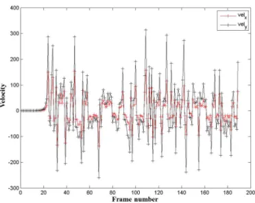
Figure 2.3: High velocity inputs to robot.
Using the standard form of navigation functions, the robot receives navigation inputs of unpredictable magnitude. Red lines showx inputs and black lines showy direction inputs.
velocity inputs and black lines representing y velocity inputs. As seen for this trial,
and typically observed in most trials, these values were found to be very high, in the hundreds or greater. Such inputs are not directly usable as an input to a practical
mobile robotic platform during experiments. Finding the right combination ofk and
K was found to be a time consuming process with no real payoff at the end in terms
of getting a usable velocity control input for the mobile robot. Hence, an improved control input was desirable for this form of the navigation function path planner.
Such an input is proposed in Section 2.3.
2.1.6
Star world transformation
For the original Rimon-Koditschek formulation to be usable in a practical workspace, the workspace has to satisfy the definition of a ‘star world’. A workspace is defined to be a star world if it contains a point called a ‘center point’ in [61]. Rays
Figure 2.4: Transformation from a star world to a circular world.
The “star world” shape to the left contains a center point which is marked by the red dot. Orange dotted lines indicate that rays emanating from the center point intersect the
workspace envelope only once. To use navigation functions for this workspace, a transformation to the circular workspace to the right needs to be estimated.
drawn to all points on the boundary of the workspace from the center point must
intersect the boundary once and only once (Figure 2.4). If the workspace is shown
to have such a center point within it, then it can be transformed to a circular world. Navigation functions can only be used in worlds which are circular and which contain circular objects.
The problem with using star world transformations is that they mandate two features for any practical workspace before they can be used in navigation function path planning:
• The workspace has to be a star world, i.e. there has to be a certainty that a
center point exists. This cannot be guaranteed for all practical workspaces.
• The transformation requires an implicit shape representation for the star world.
Such a parametric representation of the practical workspace may not be avail-able during an experimental trial.
In Section 2.4, a practical workspace representation is proposed such that the need
for computing this potentially complicated transform is removed.
the classic navigation function path planner. In subsequent sections, various mod-ifications to navigation function path planning are proposed. These modmod-ifications address the limitations of the approach outlined in the chapter introduction and in this section.
2.2
Development of an elliptical repulsion function
The first of the limitations of navigation function path planners is that obstacle motion is not encoded in them in any manner. In its original form, obstacle repulsion
is defined by Eq. (2.4). The original definition of βi satisfies the requirements of
the repulsion function from Section 2.1.2 and has the favorable property that beta
changes quadratically as the robot moves toward the obstacle. This rate of change ensures that the robot’s approach to an obstacle’s current position is strongly repelled. However, this definition does not account for the manner in which an obstacle has been moving or is expected to move. It does not convey the level of threat posed by an obstacle to the robot’s approach to the goal. For example, even if the current position of the obstacle is not between the robot and the goal, is there a chance that the obstacle will move in between the robot and target at a later instant, when the robot has moved dangerously close to the obstacle? A solution to this is to represent the obstacle motion using an elliptical field. This concept was first introduced our work [79], and has since been subject to rigorous mathematical treatment by Filippidis
and Kyriakopoulos [76], in which it was shown that the entire elliptical envelope can
Figure 2.5: Transition from circular to elliptical field.
The red circle represents the obstacle’s physical envelope. Various blue ellipses around it demonstrate the model used to encapsulate the obstacle’s predicted motion direction and
velocity.
2.2.1
Using an ellipse to create a predictive field
The original beta function for obstacles in (2.4) is modified to incorporate
information about the motion and expected future state of an obstacle. As
demon-strated in Section2.2.4, this new formulation makes the robot more responsive to the
threat posed by the motion of an obstacle, and it skews the gradient of the naviga-tion funcnaviga-tion in such a way that the region in which the obstacle may be expected to appear is avoided by the robot. To begin the discussion, consider a general ellipse equation:
[(x−he) cos(θ) + (y−ke) sin(θ)]2
a2 +
[−(x−he) sin(θ) + (y−ke) cos(θ)]2
b2 = 1 (2.7)
centered at (he, ke) and fully containing the obstacle. θ is the angle of the ellipse
major axis with respect to thexaxis. a andb are lengths of the semi-major axis and
semi-minor axis respectively.
Then the obstacle’s motion is captured using the ellipse from Eq. (2.7). This
ellipse is defined to the ‘predictive field’ of the obstacle, with the lengths of the major axis 2a and the minor axis 2b of the ellipse representing one aspect of obstacle
motion information each. When the obstacle is either known to be stationary or nothing is known about its motion, the ellipse collapses into a circle the size of the obstacle to indicate no motion information. As we learn (based on estimates from the vision system) the motion of the obstacle, the circle is skewed in the direction of motion. Therefore, the direction of the major axis indicates the estimated direction of motion, and the length of the major axis indicates the estimated speed. The length of the minor axis then indicates the uncertainty in the direction estimate. Thus, various scenarios are captured by the construction of this elliptical field, enabling it to explain the influence of predictive fields in potential field based path planning. Typical evolution of the elliptical field is illustrated in Figure2.5.
It is assumed that sensors and algorithms working in parallel with the path planner can track objects, quantify their behavior, and uses this data to provide
suitable values of a and b to guide the path planner. In case the sensing system is
not sufficiently sophisticated to provide these values, a fixed-size ellipse could also be used on the basis of motion history.
2.2.2
Constraints on the size of the ellipse
The elliptical predictive field is an estimate of where we expect the obstacle to be at a future time instant. This estimate should obviously contain the current position of the obstacle, so its radius should not extend outside the perimeter of the ellipse. If the obstacle of radiusro is placed at the focus of the ellipse, then this means
that the radius of the obstacle should be less than the periapsis (the smallest radial distance) of the ellipse:
ro ≤a− √
which rearranging terms yields a constraint on the length of the minor axis:
b≥pro(2a−ro).
The limiting case of (2.8) is when the ellipse is a circle, i.e., a =b. This leads to the following constraint on the length of the major axis:
a≥ro.
2.2.3
Formulation of repulsion function
Now that the elliptical field has been defined to capture motion trends of an object, the repulsive term in (2.4) needs a redefinition to leverage this information. It needs to be noted that the ellipse is a likely region for the presence of the obstacle, and the robot is allowed to be inside the ellipse as long as the robot does not touch
the measured position of the obstacle. The requirement that βi should go to zero
on physical contact between the robot and obstacle still needs to be obeyed, and the robot should be repelled from the obstacle at any other position in the workspace, whether inside or outside the ellipse.
In addition to the above observations, the following requirements are intro-duced for beta redefinition:
• The elliptical predictive field should provide the obstacle’s repulsive force when the robot is outside the ellipse.
• The circular formulation from Eq. (2.4) should come into play only when the
A modified beta function is proposed as follows: βi =
0 robot touches the boundary of an obstacle
βci robot is inside the ellipse
βei robot is outside the ellipse
(2.9)
where βei is the beta function for the robot with respect to the ellipse around the ith
obstacle. The obstacle is located at one focus of the ellipse defined in Eq. (2.7). Let
this position be qoi. The obstacle is expected to move along the major axis in the
direction of motion to arrive at its predicted position q′
oi at a future time instant t′.
Figure 2.6: A sample robot approach to obstacle ellipse.
Overlapping green circles indicate a sample approach path of the robot. The obstacle position (red circle) is projected along the major axis of the ellipse to its predicted position (black circle). When outside the ellipse, the black circle is used for computing obstacle repulsion term. When the robot enters the uncertain elliptical field, the actual
position of the obstacle is used to compute obstacle repulsion.
Then βei is defined as βei(q) = q−qoi′ 2 −(r+dei)2+δ, (2.10)
where dei is the distance from the predicted obstacle position qoi′ to the point qrei
where the line joining the robot position q and the predicted position of the
obsta-cle q′
oi intersects the ellipse. Various positions of the robot (indicated by the green
intersecting circles) as it approaches the obstacle along a straight line are plotted in Figure2.6. The left focus of the ellipse (red) is the actual obstacle position, the right focus (black) is the most likely predicted position. Points of intersection with the ellipse are calculated and the point closer to the robot is selected forβecomputation.
Note that if we set δ = 0, this formula for βei guarantees that it goes to zero
when the robot touches the outside of the ellipse. The curve described by this formula (with a nonzero δ) can be seen in Figure 2.7. We will see later how to define δ.
0 5 10 15 20 25 30 35 0 100 200 300 400 500 600
x − Distance between robot and obstacle
β
βe:Repulsion from ellipse βc:Repulsion from obstacle
δ x=r b x=r o+rz βc βe
Figure 2.7: Repulsion term v. robot distance from obstacle ellipse.
The requirement for the overall beta βi is that it should be defined up to
the point of contact with the obstacle. To satisfy this, the constant δ allows βei to
reduce to a non-zero minimum at the point where the robot touches the ellipse. This
constant is also the value of βci at the point where the robot touches the ellipse. As
desired. Theβci curve should be continuous with respect to theβei curve to make the
resultant beta differentiable throughout its domain. This curve is plotted in Figure
2.7.
The requirements of the function βci are:
• The function should reach its maximum value at the boundary of the ellipse,
i.e., when q−qoi′
= (r+dei).
• The function should reach its minimum value of zero when the robot and the
obstacle touch, i.e., when kq−qoik= (r+roi).
• The maximum value of the function should be given by the βci value when the
robot touches the ellipse along a straight line approach to the obstacle. Let this point beqrei. This gives δ a constant value relative to the line of approach
δ =kqrei −qoik2 + (r+roi)2. This constant value is added to the ellipse beta
when the robot is outside the ellipse, and accounts for the movement of the robot inside the elliptical predictive field.
• Additionally, the addition of delta to βei ensures that the obstacle beta
con-straint, i.e., beta goes to zero only when the robot and obstacle physically touch, is satisfied even with the addition of the ellipse to the formulation.
This is accomplished by using a mirror image of the bump function [86], since the
highest point on the curve needs to be further away from the x axis. Given the above constraints, let the following terms be defined:
rb = kqrei−qoik −(roi +r)
hc = roi +r
where:
• rb - range of the bump function, or the x coordinate where it attains its
maxi-mum
• hc - zero point of the bump function relative to distance of the robot from
obstacle
• δ - maximum value of the bump function, added to the ellipse beta
An additional point has to be made about qrei. Outside the ellipse, the point
of intersection of the robot and the ellipse, of the two possible points of intersection, is the one closer to the robot. To calculate the bump function value inside the ellipse, the definition of the point of intersection needs a slight change. As the robot moves closer and closer to the obstacle, it is possible that the point of intersection on the other side of the obstacle is the nearer point of intersection of the robot path with the ellipse. Retaining the ‘nearest intersection point’ definition will then changeδ for
the bump function and the desired shape of the β curve will be lost. To ensure this
does not happen, the unit vector from the obstacle to the robot, ¯nrei, is used. The
point of intersection is then defined as the one which is along the vector ¯nrei.
The bump function is then defined as:
βci(x) = 1 rb ≤x 0 0≤x < hc δ 2 h 1−cosπx−hc rb−hc i hc ≤x < rb (2.11)
The bump function then gets the following values. At x=hc, the obstacle and robot
touch and βci goes to zero. At x = rb, the elliptical predictive field and the robot
βci term, δ, adds to the βei term which begins to dominate the overall β function.
Therefore the value of βei approaches δ instead of 0 as the robot moves towards the
ellipse.
With these definitions for βci and βei, the overall definition of βi (2.9) is
con-sistent with the requirements of the repulsion function. In the next section, the qualitative effect of this redefinition of the repulsive term on robot navigation can be seen.
2.2.4
Effect of new repulsion function on robot path
−30 −20 −10 0 10 20 30 −30 −20 −10 0 10 20 30 →Figure 2.8: The path of the robot without predictive information.
The robot path, indicated by blue circles, approaches the obstacle path, indicated by a black dotted line, in the absence of predictive field information. The moving obstacle moves left to right, from the left end of the black dotted line, to the right, and its start and end positions are both shown by red circles. A stationary obstacle, shown by a red
circle, sits at (−20,8) throughout the simulation.
MATLAB Simulink (Mathworks Inc., Natick, MA) was used to simulate the proposed change to the repulsion function and to qualitatively compare it against previous results from Chen et al. ([72, 84, 85]). Such a comparison is easily possible because the predictive field reduces to the obstacle’s circular envelope when motion
information is not used, and Eq. (2.10) reduces to Eq. (2.4). The hypothesis to be
tested is: using predictive fields makes it possible for the robot to converge to the target following more effectively than using the original navigation function formula-tion from Rimon and Koditschek. This also implies that the robot is pushed away from the predicted path of the obstacle, thus driving it to goal using a less dangerous
−30 −20 −10 0 10 20 30 −30 −20 −10 0 10 20 30 →
Figure 2.9: The path of the robot with predictive information.
The setup of this figure is exactly the same as Figure2.8. The robot path, indicated by blue circles, moves away from the obstacle path, indicated by a black dotted line, when predictive field information is used. Elliptical field of the moving obstacle is indicated by
the blue envelope around the red circle representing it.
route. This notion of ‘danger’ of collision with obstacles has also been explored in the context of potential fields path planning [82, 81,80].
Results are demonstrated using two hypothetical scenarios:
1. An obstacle initially obstructs the straight line path from robot to goal, but it begins to move out of the way as the simulation progresses.
2. An obstacle is initially at a distance from the straight line trajectory from robot to goal, but it moves to obstruct the path as the simulation progresses.
Both cases are tested with and without the predictive predictive field sur-rounding the obstacle. The setup of the workspace is described as follows:
• The workspace envelope bump function comes into effect at a distance rs= 5. • Goal is located at (−10,20).
• Stationary obstacle with radius ro1 = 3 is located at (−20,8). The stationary
nature of the obstacle causes the predictive predictive field around it to shrink to a circle with the same radius as the obstacle.
• The workspace is centered at (0,0) with a radius of ro0 = 35.
• The predictive field of the moving obstacle of radius ro2 = 3 is described by an
ellipse with parameter a= 8 in both cases.
• Gains from Eq. (2.1) and Eq. (2.6) are set atκ= 4.5 andK = 1.2 respectively. They remain unchanged for the given setup; however, they might need to be tuned on changing the number of obstacles in the workspace.
In Scenario 1, the obstacle starts at (−20,0) and travels 20 units in the
workspace at a constant velocity. The sense of its motion is such that it is mov-ing out of the way of the robot’s path to goal. Without the use of a predictive field,
it can be seen that, in Fig. 2.8, the robot tries to move around the obstacle. This
causes it to move toward the path of the obstacle and forces a correction in its path approximately midway through its trajectory. However, when the predictive field is added, the path planner is able to sense that the more optimal path to goal would actually be behind the obstacle, as seen in Fig. 2.9. The trajectory traced as a result is much more intuitive than the first case.