Approximations for the likelihood ratio statistic for hypothesis testing between two Beta distributions.

Durham Research Online

Deposited in DRO:

16 October 2018

Version of attached le:

Peer-review status of attached le:

Citation for published item:

Marques, F.J. and Coolen, F.P.A. and Coolen-Maturi, T. (2019) 'Approximations for the likelihood ratio statistic for hypothesis testing between two Beta distributions.', Journal of statistical theory and practice., 13 . p. 17.

Further information on publisher's website:

Publisher's copyright statement:

This is a post-peer-review, pre-copyedit version of an article published in Journal of statistical theory and practice. The nal authenticated version is available online at: https://doi.org/10.1007/s42519-018-0021-8

Additional information:

Use policy

The full-text may be used and/or reproduced, and given to third parties in any format or medium, without prior permission or charge, for personal research or study, educational, or not-for-prot purposes provided that:

• a full bibliographic reference is made to the original source • alinkis made to the metadata record in DRO

• the full-text is not changed in any way

The full-text must not be sold in any format or medium without the formal permission of the copyright holders. Please consult thefull DRO policyfor further details.

Approximations for the likelihood ratio statistic for

hypothesis testing between two Beta distributions

Filipe Marques,

Email: [email protected]

Frank Coolen,

Durham, UK.

Email: [email protected]

Tahani Coolen-Maturi,

Durham, UK.

Email: [email protected]

Abstract

In this paper the likelihood ratio to test between two Beta distributions is addressed. The exact distribution of the likelihood ratio statistic, for simple hypotheses, is ob-tained in terms of Gamma or Generalized Integer Gamma distributions, when the first or the second of the two parameters of the Beta distributions are equal and integers. In the remaining cases addressed, near-exact or asymptotic approximations, are developed for the likelihood ratio statistic. Both the exact, asymptotic or near-exact representa-tions are obtained using a logarithm transformation of the likelihood ratio statistic and by working with the corresponding characteristic function. The numerical studies il-lustrate the precision of the approximations developed. Simulations are developed to analyse the power and the reproducibility probability of the tests.

AMS Subject Classification: 62F03,62E15,62E20,62G99

Keywords: Likelihood ratio tests, Generalized Integer Gamma distribution, General-ized Near-Integer Gamma distribution, Mixtures, Reproducibility probability, Non-parametric predictive inference

1 Introduction

In this work we consider the likelihood ratio to test between two completely speci-fied Beta distributions. The Beta distribution is an important tool for many statistical

problems with applications in different areas. As examples we point out the following features; i) thei-th order statistic of a sample of sizen, extracted from a continuous uni-form distribution, has a Beta distribution, ii) in Bayesian statistics it is commonly used as conjugate prior for binomial and geometric random variables, iii) it is the distribu-tion of Wilks’s lambda in some particular cases and iv) in the general case, the Wilks’s lambda distribution can be related with the product of independent Beta random vari-ables. The test addressed in this work, is a useful procedure in the decision making between two Beta distributions, thus may be helpful in problems arising from the pre-vious examples, such as in the Bayesian framework in the selection, between two Beta models, of the conjugate prior distribution of the probability of success of a Binomial or Geometric distribution. Some possible applications of this Bayesian approch may be found in biological assays, medicine (Gupta and Nadarajah, 2004; Griffiths, 1973; Pham et al., 2010), in social sciences (Wiley et al., 2015) and in financial problems (Rachev et al., 2008). We say that a random variableX has a Beta distribution with parametersa >0andb >0, and we denote this fact byX∼Beta(a, b), if its density function is given by

f(x) = 1

B(a, b)x

a−1_(1−x)b−1_{, with 0≤x≤1}

whereB(., .)denotes the usual beta function. For a sample of sizen,X1, . . . , Xn, we

consider the following simple hypotheses

H0:Xi∼Beta(a, b) vsH1:Xi∼Beta(c, d) (1)

and we study the following cases: I)b = d = 1or a = c = 1, II)b = d = αor

a=c =αwithα∈_N, III)a=c=rorb =d=rwithr ∈_R\_N, IV)a−c∈_N

andb−d∈_N, and finally V) the general case with no restrictions on the parameters. In cases I and II the exact distribution is presented in terms of Gamma or Generalized Integer Gamma (GIG) distributions (Coelho, 1998). In case III, near-exact approxima-tions (Coelho, 2004) are developed for the likelihood ratio statistic. These near-exact approximations are developed by working with the characteristic function of the log-arithm of the likelihood ratio statistic. More precisely, first an adequate factorization of the expression of the characteristic function is obtained, and then one of the factors is approximated in such way that the resulting characteristic function corresponds to a known and manageable distribution. In cases IV and V, asymptotic approximations, based on shifted mixtures of (positive or negative) Gamma distributions are obtained for the likelihood ratio statistic. These approximations allow the computation ofp -values and quantiles in a fast and precise way. Thus, using the approximations devel-oped in Subsections 2.3-2.5, other more complex and time consuming techniques may be avoided to determine quantiles, such as numerical inversion formulas together with bisection methods or simulations. We should also point out that Wilks theorem (Wilks, 1983) which states that the distribution of the logarithm of likelihood ratio test statistics used to test composite hypotheses can be approximated by aχ2_{distribution can not be}

used when both hypotheses are completely specified, since in this case the number of degrees of freedom under the alternative and null hypotheses is equal to zero. This reinforces the importance of having approximations which may allow to perform these tests with the appropriate accuracy.

This work is organized as follows. In Section 2, five cases are considered; four with conditions on the parameters of the Beta distributions involved, and one with no restrictions on the parameters. In Section 3, the power and reproducibility of the test are illustrated with simulation studies. Section 4 is dedicated to the concluding remarks. 2 The likelihood ratio statistic and its distribution

For a random sample of sizen,X1, . . . , Xn, we are interested in a test which may allow

two decide between two Beta distributions with the parameters completely specified. The hypotheses of interest are defined in (1) .

The likelihood ratio statistic is given by

Λ = n Y i=1 f0(xi) f1(xi)

wheref0(.)andf1(.)are the probability density functions of two Beta random

vari-ables with distributionsBeta(a, b)andBeta(c, d). Thus, the likelihood ratio may be written as Λ = n Y i=1 B(c, d)x_ia−1(1−xi)b−1 B(a, b)x_ic−1(1−xi)d−1 = _{B(c, d)} B(a, b) n n Y i=1 xa_i−c(1−xi)b−d.

To study the null distribution ofΛ, underH0in (1), we are essentially interested in the

distribution ofQn_i=1X_ia−c(1−Xi)b−d, forX1, . . . , Xn independent and identically

distributed asXi∼Beta(a, b).

2.1 Case I:b=d= 1ora=c= 1

Forb=d= 1we are interested in testing

H0:Xi ∼Beta(a,1) vs H1:Xi∼Beta(c,1).

The expression ofΛ, for an observed sample of sizen, is given by

Λ = n Y i=1 a c x a−c i = a c n_Yn i=1 xa_i−c.

This case was already addressed in Marques et al. (2018), however for completeness of this work we present it here with more detail, for example, now we specify the cases

a−c >0andc−a >0.

Theorem 2.1 If X1, . . . , Xn are independent and identically distributed withXi ∼

Beta(a,1)then the cumulative distribution function of

Λ =a

c

nYn

i=1

witha, c >0, is i) fora−c >0 1−F_Γ(n, a a−c) −log _x (a/c)n (2) ii) fora−c <0 F_Γ(n,− a a−c) log x (a/c)n (3) whereFΓ(r,λ) is the cumulative distribution function of a Gamma distribution with shape parameterr >0and rate parameterλ >0.

Proof Let us considerX1, . . . , Xnindependent and identically distributed withXi ∼

Beta(a,1)and the random variableW =−log(Qn_i=1X_ia−c) =Pn_i=1−(a−c) log(Xi).

Since we know that−log(Xi)has an exponential distribution with parametera, theh

-th moment ofX_ia−cis given by

EhX_i(a−c)hi= a

a+h(a−c)

and, given the relationE

eitW

=E

Λ−it

, the expression of the characteristic func-tion of−(a−c) log(Xi)is given by

Φ−(a−c) log(Xi)(t) = a a−it(a−c).

Ifa−c >0, then, we may say that the characteristic function ofW is given by

ΦW(t) = a a−c a a−c−it !n .

This is the characteristic function of a Gamma distribution with shape parameternand rate parameter_a−a_c. Therefore it is easy to show, with the necessary transformations, that the cumulative distribution function ofΛwhena−c >0is given by

1−F_Γ(n, a a−c) −log _x (a/c)n .

Following a similar procedure it is possible to obtain the result stated fora−c <0, we just have to note that, fora−c <0

ΦW(t) = a c−a a c−a+ it !n .

This is the characteristic function of a negative Gamma random variable. Again, after simple transformations we obtain the expression

F_Γ(n,− a a−c) log _x (a/c)n .

Please note that:

1. if one considers the casea=c= 1, andb−d >0ord−b >0

H0:Xi∼Beta(1, b) vsH1:Xi∼Beta(1, d)

the expression ofΛ, for a sample of sizen, is given by

Λ = n Y i=1 b d(1−xi) b−d_,

and using the mirror property of the beta distribution if one takesX1, . . . , Xn

independent and identically distributed fromBeta(1, b)we know that1−Xi ∼

Beta(b,1), and thus this case is the same as the previous one;

2. clearly, the result in Theorem 2.1, is obtained under the null hypothesis, however the distribution of the likelihood ratio statistic under the alternative hypothesis is obtained following the same procedure.

These last notes also apply to the following cases considered.

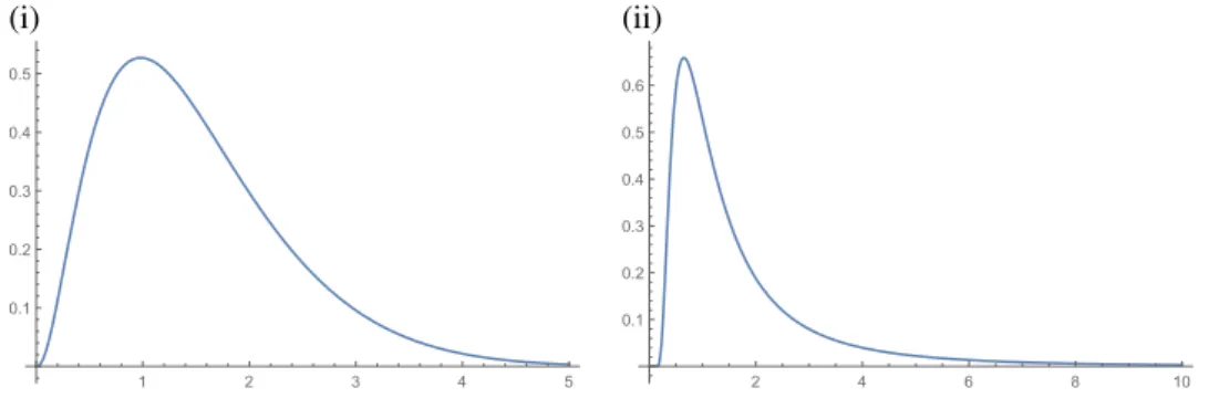
Just as an illustration we present, in Figure 1, plots of the density functions corre-sponding to the distributions derived in Theorem 2.1, for two different scenarios: (i)

a=1₄,c= 1₅andb=d= 1and (ii)a= 4,c= 5andb=d= 1.

Figure 1: Plots of the probability density functions, for the first case, in the following scenarios: (i)a= 1₄andc=1₅, (ii)a= 4andc= 5

(i) (ii) 1 2 3 4 5 0.1 0.2 0.3 0.4 0.5 2 4 6 8 10 0.1 0.2 0.3 0.4 0.5 0.6

2.2 Case II:b=d=αora=c=αwithα∈N

Forb=d=α, withα∈N, we consider the hypotheses

The expression ofΛ, for an observed sample of sizen, is given by Λ = _{B(c, α)} B(a, α) n n Y i=1 xa_i−c.

Although the expression of the likelihood ratio statistic is similar to the one in Subsec-tion 2.1, since the underlying populaSubsec-tions may be different (ifα >1), the distribution ofΛ, under the null hypothesis, will also be different.

Theorem 2.2 If X1, . . . , Xn are independent and identically distributed withXi ∼

Beta(a, α), witha >0andα∈N, the cumulative distribution function of

Λ = _{B(c, α)} B(a, α) n n Y i=1 X_ia−c

withc >0, is (using the notation in Appendix 1 of Marques et al. (2015) for the GIG distribution) i) fora−c >0 1−FGIG  −log   x _B(c,α) B(a,α) n  ;n, v, α   with n={n, . . . , n}1×α, v= _{a+ 0} a−c, . . . , a+α−1 a−c 1×α (4) ii) fora−c <0 FGIG  log   x _B(c,α) B(a,α) n  ;n,−v, α  

whereFGIG(.)denotes the cumulative distribution function of a Generalized Integer Gamma (GIG) distribution (Coelho, 1998) with integer shape parametersnand rate parametersvgiven in (4) .

Proof Similar to the proof of Theorem 2.1, we considerX1, . . . , Xn independent

and identically distributed random variables withXi ∼ Beta(a, α)and the random

variableW = −log(Qn_i=1X_ia−c) = Pn_i=1−(a−c) log(Xi). It is known that the

characteristic function ofW is given by

ΦW(t) = n Y j=1 Γ(a+α) Γ(a) Γ(a−(a−c)it) Γ(a+α−(a−c)it) = _Γ(a+α) Γ(a) Γ(a−(a−c)it) Γ(a+α−(a−c)it) n .

Sinceα∈_Nand using the following equality, forz∈_C

Γ(z+α) Γ(z) = α−1 Y k=0 z+k (5)

we may write ΦW(t) = α−1 Y k=0 (a+k)(a+k−(a−c)it)−1 !n = α−1 Y k=0 a+k a−c a+k a−c −it !n . (6)

Whena−c >0, the characteristic function in expression (6) corresponds to the sum of αindependent Gamma distributions, all with integer shape parameters, that is a GIG distribution with shape parameters given byn={n, ..., n}1×αand rate

parame-tersv =na_a+0_−c, . . . ,a+_aα₋−_c1o

1×α. After the necessary transformations the cumulative

distribution function ofΛis given by

1−FGIG  −log   x _B(c,α) B(a,α) n  ;n, v, α  .

Whena−c <0, expression (6) can be written as

ΦW(t) = α−1 Y k=0 a+k −a+c a+k −a+c+ it !n

which is the characteristic function of a random variableY such that−Y has a GIG distribution with shape parameters given byn = {n, ..., n}1×αand rate parameters −v=n₋a_a+0_+c, . . . ,a₋+_aα₊−_c1o

1×α

. In this case the cumulative distribution function ofΛ

is given by FGIG  log   x _B(c,α) B(a,α) n  ;n,−v, α  .

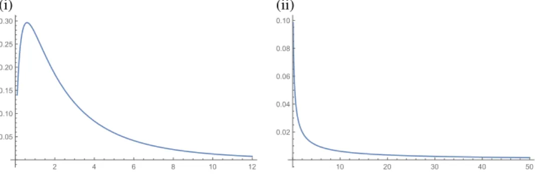
In Figure 2 we present the probability density functions corresponding to the distribu-tions in Theorem 2.2 for two scenarios: (i)a= 2,c = 3/2,b=d= 3, (ii)a= 7/5,

c= 3,b=d= 3.

Results for the casesa =c =α,b−d > 0 orb−d < 0may be obtained in a similar way.

2.3 Case III:b=d=rora=c=rwithr∈_R\_N

Similar to what was done in the previous section, we will just address one of the cases. Forb=d=rwithr∈R\N, we consider

H0:Xi∼Beta(a, r) vs H1:Xi ∼Beta(c, r)

the expression ofΛ, for an observed sample of sizen, is given by

Λ = _{B(c, r)} B(a, r) n n Y i=1 xa_i−c.

Figure 2: Plots of the probability density functions, for the second case, in the following scenarios: (i)a= 2,c= 3/2,b=d= 3, (ii)a= 7/5,c= 3,b=d= 3

(i) (ii) 2 4 6 8 10 12 0.05 0.10 0.15 0.20 0.25 0.30 10 20 30 40 50 0.02 0.04 0.06 0.08 0.10

In this case we do not have the exact cumulative distribution function ofΛin a manage-able expression but we will show how it is possible to obtain precise approximations. We consider independent and identically distributed random variables X1, . . . , Xn

withXi∼Beta(a, r)and the random variable

W =−log n Y i=1 X_ia−c ! = n X i=1 −(a−c) log(Xi).

The characteristic function ofW is given by

ΦW(t) = n Y j=1 Γ(a+r) Γ(a) Γ(a−(a−c)it) Γ(a+r−(a−c)it). (7)

Ifr > 1we may develop near-exact approximations for the distribution of the likeli-hood ratio statistic. These approximations, introduced by Coelho (2004), have already been used in several works involving the study of the distribution of likelihood ratio statistics used to test the structure of covariance matrices in the multivariate setting (Coelho et al., 2010; Coelho and Marques, 2012; Marques et al., 2017). The process may be illustrated as follows. The characteristic function in (7) may be factorized as follows ΦW(t) = _Γ(a+r?₎ Γ(a) Γ(a−(a−c)it) Γ(a+r?_{−(a−c)it)} n_Γ(a+r) Γ(a+r?₎ Γ(a+r?_{−(a−c)it)} Γ(a+r−(a−c)it) n (8)

with integerr?=brc. Using the equality in (5) we may write ΦW(t) = r?₋₁ Y k=0 a+k a+k−(a−c)it !n _Γ(a+r) Γ(a+r?₎ Γ(a+r?−(a−c)it) Γ(a+r−(a−c)it) n = r?₋₁ Y k=0 a+k a−c a+k a−c −it !n | {z } ΦW1(t) _Γ(a+r) Γ(a+r?₎ Γ(a+r?_{−(a−c)it)} Γ(a+r−(a−c)it) n | {z } ΦW2(t) . (9)

The characteristic functionΦW1 in (9) corresponds to the characteristic function of a

GIG distribution with shape parameters given byn={n, ..., n}1×r?and rate

parame-tersv=na+0

a−c, . . . , a+r?−1

a−c o

1×r?. The characteristic functionΦW2in (9) corresponds

to the sum ofnindependent Logbeta random variables, multiplied bya−c, with param-etersa+r?andr−r?. As a basis for the development of the near-exact approximations we consider the expansion for the ratio of Gamma functions given in expressions (11)– (14) of Tricomi and Erd´elyi (1951) or in expression (12) of Luke (1969) which may be used to show that a Logbeta distribution may be represented as an infinite mixture of Gamma distributions. Thus, we propose as an approximation for the characteristic functionΦW2in (9) the characteristic function of a mixture ofm?+ 1Gamma

distribu-tions, all with rate parameterλand with shape parametersr+j,j= 0, . . . , m?_given

by ΦW? 2(t) = m? X j=0 πjλs+j(λ−it)−(s+j). (10)

Following the results in Coelho et al. (2010) we definesequal to the sum of the second parameters of the Logbeta distributions involved in the characteristic function ofΦW2

in (9)

s=n(r−r?). (11) Then, the process has two main steps, first the parameterλis determined as the rate parameter of a mixture of two Gamma distributions which equates the first 4 moments of the exact distribution ofW2, and second, assuming a fixed value forλ, the weights,

πj, are determined ensuring that the approximating distribution equates the firstm?

exact moments, being thus the weights,πj(j= 0, . . . , m?−1), obtained as a solution

of the system ∂h ∂thΦW2(t) _t=0 = ∂ h ∂thΦW2?(t) _t=0 , h= 1, . . . , m?, (12) withπm?= 1−Pm ?₋₁

j=0 .The resulting approximating characteristic function is given

by

ΦW?(t) = Φ_W1(t)×Φ_W?

and corresponds to a mixture Generalized Near-Integer Gamma (GNIG) distribution (Coelho, 2004) with weightsπjand with the GNIG parameters given by

nj = {n, ..., n, s+j}1×(r?₊₁₎ withj= 0, . . . , m? andsin (11) (13) v = _{a+ 0} a−c, . . . , a+r?₋₁ a−c , λ 1×(r?+1) . (14)

Using the notation in Appendix 1 of Marques et al. (2015), the corresponding approx-imating cumulative distribution function forΛmay be represented as

1− m? X j=0 πjFGNIG  −log   x _B(c,r) B(a,r) n  , n_j, v, r?+ 1  . (15)

Ifa−c <0, then the procedure to develop near-exact approximations for the distribu-tion of the likelihood ratio statistic is similar to the previous one, but the approximating distributions will correspond to mixtures of negative GNIG distributions with weights

πj determined as solutions of the system of equations in (12) and the negative GNIG

distributions with parameters given byn_jin (13) and−vwithvgiven in (14). The previous results may be summarized in the following theorem.

Theorem 2.3 If X1, . . . , Xn are independent and identically distributed withXi ∼

Beta(a, r),a >0,r∈R\Nandr >1, and by approximatingΦW2 in (9) byΦW2?in

(10) we obtain for Λ = _{B(c, r)} B(a, r) n n Y i=1 X_ia−c

withc >0, near-exact cumulative distribution functions given by i) fora−c >0 1− m? X j=0 πjFGNIG  −log   x _B(c,r) B(a,r) n  , n_j, v, r?+ 1  

and, ii) fora−c <0

m? X j=0 πjFGNIG  log   x _B(c,r) B(a,r) n  , nj,−v, r ? + 1  

whereFGNIG(.)denotes the cumulative distribution of a GNIG distribution (Coelho, 2004) with shape parametersn_jin (13) and rate parametersvin (14) . The weightsπj

are obtained as solution of the system of equations in (12).

Ifr < 1, then the approximation is obtained using a similar approach but for the characteristic functionΦW in (8), making s = rn andλas the rate parameter of a

distribution ofW and the weightsπj as the solution of the system of equations given

in (12) replacingΦW2 byΦW. The resulting approximation is a simple mixture of

Gamma distributions.

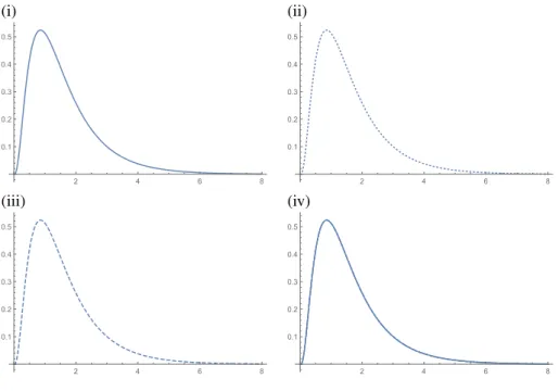
To illustrate the precision of these approximations, in Figure 3 we present for sce-narioa = 17/5,r = 9/4,c = 3andn = 20the plots for: (i) the exact probability density function, obtained using the inversion formulas in Gil-Pelaez (1951), (ii) the near-exact probability density function obtained form?_{= 2, (iii) the near-exact}

proba-bility density function obtained form?_{= 4and (iv) the representation in the same plot}

of (i), (ii) and (iii). The use of the inversion formulas in Gil-Pelaez (1951) is somehow limited. For example, if one wants to determine the exact quantiles ofΛwe have to use these formulas together with the bisection method and this process may require a high computing time. Moreover, in the following subsections with more complex scenarios we were not able to plot the exact densities with the inversion formulas in Gil-Pelaez (1951). In Figure 3, the differences between the exact and approximating densities are indistinguishable even for small values ofm?_{such as 2 and 4.}

Figure 3: Plots of the probability density functions, for Case III, scenarioa= 17/5,

r= 9/4,c= 3andn= 20, of the (i) the exact probability density function, obtained using the inversion formulas in Gil-Pelaez (1951), (ii) the near-exact probability density function obtained form?_{= 2, (iii) the near-exact probability density function obtained}

form?_{= 4and (iv) the representation in the same plot of (i), (ii) and (iii).}

(i) (ii) 2 4 6 8 0.1 0.2 0.3 0.4 0.5 2 4 6 8 0.1 0.2 0.3 0.4 0.5 (iii) (iv) 2 4 6 8 0.1 0.2 0.3 0.4 0.5 2 4 6 8 0.1 0.2 0.3 0.4 0.5

2.4 Case IV:a−c∈Nandb−d∈N

Fora−c∈Nandb−d∈N, we consider the hypotheses

H0:Xi∼Beta(a, b) vsH1:Xi∼Beta(c, d)

and the expression ofΛ, for an observed sample of sizen, is now given by

Λ = n Y i=1 B(c, d) B(a, b)x a−c i (1−xi)b−d.

This is a more complex case, for which we will only be able to derive asymptotic approximations for the distribution ofΛ. The procedure is as follows. Let us consider independent and identically distributedX1, . . . , Xn withXi ∼Beta(a, b)anda, b >

0.

Just as a side note we point out thatXi/(1−Xi)has a beta prime distribution, so

ifb−d <0such thatb−d=−(a−c)we have as particular case

Λ = _{B(c, d)} B(a, b) n n Y i=1 X_ia−c(1−Xi)−(a−c) = _{B(c, d)} B(a, b) n n Y i=1 _X i 1−Xi a−c

where we may identify the product of beta prime independent random variables to the powera−c.

Considering again the case addressed in this subsection, we have

Λ = _{B(c, d)} B(a, b) n n Y i=1 X_ia−c(1−Xi)b−d, (16)

witha−c∈N,b−d∈Nanda,b,canddpositive real numbers. The characteristic

function of−log{X_ia−c(1−Xi)b−d}is given by

Γ(a−(a−c)it)Γ(b−(b−d)it)

B(a, b)Γ(a+b−(a−c)it−(b−d)it)

and as such the characteristic function of

W =−log n Y i=1 X_ia−c(1−Xi)b−d ! = n X i=1 −log{X_ia−c(1−Xi)b−d}

is, in the general case, given by

ΦW(t) =

_{Γ(a−(a−c)it)Γ(b−(b−d)it)}

B(a, b)Γ(a+b−(a−c)it−(b−d)it)

n

Given that in the particular case considered one hasa−c ∈ Nandb−d∈ N, after

some technical developments of this last expression and using the Gauss multiplication formula which, for a positive integerη, is given by

η−1 Y k=0 Γ _k η +z = (2π)η−21η 1 2−ηzΓ(ηz)

we may write the characteristic function ofW as

ΦW(t) =K1e−itK2 _a−c−1 Q k=0 Γ_a−a_c+_a−k_c−it _b−d−1 Q k=0 Γ_b−b_d+_b−k_d−it n _{a+b−c−d−1} Q k=0 Γ_a+a_b−+b_c−d +_a+b−k_c−d −it n (18)

with the constantsK1andK2given by

K1= √ 2π(a−c)a−1 2(b−d)b−12(a+b−c−d)−a−b+12 B(a, b) !n and

K2=n(−(a+b−c−d) log(a+b−c−d) + (a−c) log(a−c) + (b−d) log(b−d)).

The characteristic function in (18) may be written as

ΦW(t) = e−itK2 ×K1   a−c−1 Y k=0 Γ_a−a_c+_a−k_c−it Γ_a+a_b+_−cb_−d+_a+b−k_c−d−it   n ×   b−d−1 Y k=0 Γ_b−b_d+_b−k_d −it Γ_a+a_b+_−cb_−d+_a+k+_b−a−_c−c_d−it   n | {z } ΦW₁(t) = e−itK2_Φ W1(t). (19)

We should note that, in expression (19),K2corresponds to a shift in the main

distri-bution. In order to obtain approximations for the distribution of the likelihood ratio one will use a similar procedure to the one given in Coelho and Alberto (2012) and Marques et al. (2017). More precisely, we will approximate the characteristic function ofW1in (19) by a simple mixture of Gamma distributions, all with rate parameterλ

and with shape parametersr+j,j= 0, . . . , m?. Thus, we obtain as an approximating characteristic function ofΦW in (17) the characteristic function

ΦW?(t) = e−itK2

m?

X

j=0

whereλand the weightsπj are determined using a matching moments technique in

two steps. Firstλis determined as the solution of the following system of equations

∂h ∂thΦW1(t) _t=0 =∂ h ∂th (λ)r1_(λ−it)−r1 _t=0 (21) forh= 1,2, that is,λis the rate parameter of a Gamma distribution which matches the first 2 moments of the exact distribution ofW1and, following a same procedure as

the one used in Subsection 2.3,ris defined as

r=n (b−d−1 X k=0 k b−d+ b b−d− _a−c+k a−c+b−d+ a+b a−c+b−d ) (22) + (_a−c−1 X k=0 k a−c + a a−c− _k a−c+b−d+ a+b a−c+b−d )! .

Given the complexity of the distribution in this case and in order to improve the quality of the approximations, in some cases one will considerr = r1 given as solution of

the system in (21). Finally, assuming fixed values forλandr, the weights, πj, are

determined as a solution of the system

∂h ∂thΦW1(t) _t=0 = ∂ h ∂th m? X j=0 πjλr+j(λ−it)−(r+j) _t=0 , h= 1, . . . , m? (23) with πm?= 1− m?−1 X j=0 πj.

Thus, we have as approximating distributions ofW, mixtures of shifted Gamma butions which, by simple transformation, give rise to the following cumulative distri-bution function 1− m? X j=0 πjFΓ(r+j,λ)  −log   x _B(c,d) B(a,b) n  −K2  . (24)

This procedure is summarized in the following theorem.

Theorem 2.4 If X1, . . . , Xn are independent and identically distributed withXi ∼

Beta(a, b),a, b >0, by approximatingΦW in (17) byΦW?in (20) we obtain for

Λ = _{B(c, d)} B(a, b) n n Y i=1 X_ia−c(1−Xi)b−d,

witha−c ∈ _N, b−d ∈ _Nand a,b, cand dpositive real numbers, the following approximating cumulative distribution function

1− m? X j=0 πjFΓ(r+j,λ)  −log   x _B(c,d) B(a,b) n  −K2  

whereFΓ(r+j,λ)(.)denotes the cumulative distribution function of a Gamma distribu-tion with shape parameterr+jand rate parameterλ. The parameterλis obtained as solution of the system in (21) andris defined as in (22) or is set equal tor1which is obtained as solution of the system in (21) . The weightsπjare obtained as solution of

the system of equations in (23).

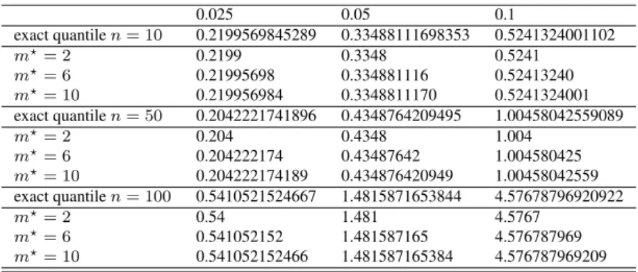
In Case IV, we were not able to plot the exact probability density functions using the inversion formulas in Gil-Pelaez (1951). Therefore, in order to illustrate the precision of these approximations we present in Table 1, the exact, 0.01, 0.05 and 0.1, quantiles of Λ computed using the inversion formulas in Gil-Pelaez (1951) and the bisection method, and the equal decimal places of the approximating quantiles, obtained using expression (24). In Table 1 we considered the following scenarios: a = 17/5, b = 16/3,c= 12/5,d= 10/3,n= 10,50,100andm?_{= 2,6,10. We would like to point}

out that the computing time needed for the proposed approximations is nearly zero.

Table 1: Comparison between exact and approximating quantiles, Case IV

0.025 0.05 0.1 exact quantilen= 10 0.2199569845289 0.33488111698353 0.5241324001102 m?_{= 2 0.2199 0.3348 0.5241} m?_{= 6 0.21995698 0.334881116 0.52413240} m?_{= 10 0.219956984 0.3348811170 0.5241324001} exact quantilen= 50 0.2042221741896 0.4348764209495 1.00458042559089 m?_{= 2 0.204 0.4348 1.004} m?_{= 6 0.204222174 0.43487642 1.004580425} m?_{= 10 0.204222174189 0.434876420949 1.00458042559} exact quantilen= 100 0.5410521524667 1.4815871653844 4.57678796920922 m?_{= 2 0.54 1.481 4.5767} m?_{= 6 0.541052152 1.481587165 4.576787969} m?_{= 10 0.541052152466 1.481587165384 4.576787969209}

The cases wherec−a ∈Nandd−c ∈N, or other possible combinations, may

also be addressed using similar procedures, but in these cases we may have to consider mixtures of shifted negative gamma distributions.

2.5 General case

Finally, having as basis the procedure described in Subsection 2.4, we propose as an ap-proximation forΛ, in the general case with no restrictions on the parameters, mixtures of shifted (positive or negative) Gamma distributions. One will approximate the char-acteristic function in (17) ofW =−log(Λ)withΛgiven in (16) with no restrictions on the parametersa, b, c, d >0, by the characteristic function of a mixture of shifted (pos-itive or negative) Gamma distributions with shape parametersr+j(j = 0, . . . , m?), rate parameterλand shift parameterw, given by

ΦW?(t) =

m?

X

j=0

The parametersr,λandwwill be determined as solutions of the system of equations ∂h ∂thΦW(t) _t=0 =∂ h ∂th (λ)r(λ−it)−reitw _t=0 (26) forh = 1,2,3. One should note that, when a−c < 0 orb−d < 0one will ob-tain a negative rate parameter, that isλ < 0, which means that in these cases one will have instead of a mixture of gamma distributions,Yj ∼Γ(r+j, λ), with a shift

parameter equal tow, a mixture of−Yj ∼Γ(r+j,−λ)distributions with the same

shift parameter. Through the system of equations in (26) we define the rate, shape and shift parameters of the gamma distributions involved, and then we move forward to determine the weights. The weights are determined for fixed values ofr,λandw, by matching a given number, let us saym?, of exact moments, that is by solving the system ∂h ∂thΦW(t) _t=0 = ∂ h ∂thΦW?(t) _t=0 , h= 1, . . . , m? (27) with πm?= 1− m?−1 X j=0 πj withΦW?in (25).

Theorem 2.5 If X1, . . . , Xn are independent and identically distributed withXi ∼

Beta(a, b),a, b > 0, by approximating the characteristic function in (17) of W =

−log(Λ)byΦW?in (25) we obtain for

Λ = _{B(c, d)} B(a, b) n n Y i=1 X_ia−c(1−Xi)b−d,

the following approximating cumulative distribution functions i)a−c >0andb−d >0 1− m X j=0 πjFΓ(r+j,λ)  −log   x _B(c,d) B(a,b) n  −w   (28) and whena−c <0orb−d <0 m X j=0 πjFΓ(r+j,−λ)  log   x _B(c,d) B(a,b) n  +w   (29)

whereFΓ(r+j,λ)(.)denotes the cumulative distribution function of a Gamma distribu-tion with shape parameterr+jand rate parameterλ. The parametersλ,randware obtained as solutions of the system in (26). The weightsπjare obtained as solution of

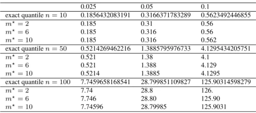
In this case, as also happened in Subsection 2.4, we were not able to plot the exact probability density functions. In Table 2 we present the exact, 0.01, 0.05 and 0.1, quantiles ofΛcomputed using the inversion formulas in Gil-Pelaez (1951), and the equal decimal places of the approximating quantiles computed using expression (28). In this table we consider the following scenarios:a= 22/5,b= 3,c= 10/3,d= 7/4,

n= 10,25,50andm?_{= 2,6,10.}

Table 2: Comparison between exact and approximating quantiles, Case V

0.025 0.05 0.1 exact quantilen= 10 0.1856432083191 0.3166371783289 0.5623492446855 m?= 2 0.185 0.31 0.56 m?_{= 6 0.185 0.316 0.56} m?_{= 10 0.185 0.316 0.562} exact quantilen= 50 0.5214269462216 1.3885795976733 4.1295434205751 m?= 2 0.521 1.38 4.1 m?_{= 6 0.521 1.388 4.129} m?_{= 10 0.5214 1.3885 4.1295} exact quantilen= 100 7.7459658168541 28.799851109827 125.90314598279 m?= 2 7.74 28.8 126. m?_{= 6 7.746 28.80 125.90} m?_{= 10 7.74596 28.79985 125.9031}

The results in Table 2, when compared with the ones in Table 1, show that the approximation developed for the general case is not as precise as the one developed for Case IV. Even so, it is a very reasonable approximation equating, in most cases, two decimal places of the exact quantile in the scenario under consideration.

3 Numerical studies and simulations

In this section, the power and the reproducibility properties of the test are illustrated through simulations.

3.1 Power study

To illustrate the power of these tests we consider the same scenarios addressed in Sub-sections 2.1 and 2.3 which are

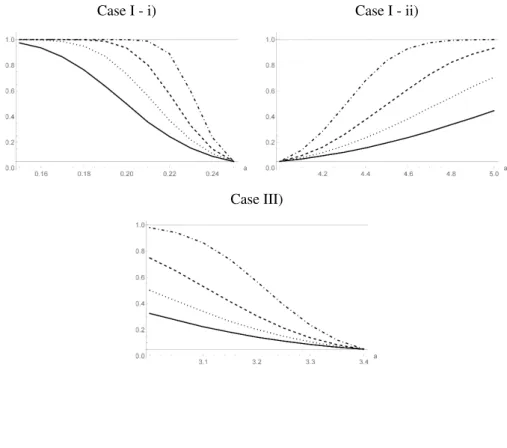
Case I - i)a= 1/4,c= 1/5andb=d= 1 (a > c)

H0:Xi∼Beta(1/4,1) vsH1:Xi∼Beta(1/5,1)

Case I - ii)a= 4,c= 5andb=d= 1 (a < c)

H0:Xi∼Beta(4,1) vsH1:Xi∼Beta(5,1)

Case III -a= 17/5,c= 3andb=d=r= 9/4

Theα = 0.05quantile was computed using the expressions of the exact cumulative distribution functions in (2) or (3) for Case I, and the near-exact cumulative distri-bution function in (15) for Case III. To compute the empirical power we considered 100 000 replications of samples of sizen= 50,100,200and500from the following distributions

Case I - i)Xi ∼Beta(a,1)withafrom 0.15 to 0.25 step 0.01

Case II - ii)Xi∼Beta(a,1)withafrom 4.0 to 5.0 step 0.1

Case III -Xi∼Beta(a,9/4)withafrom 3.0 to 3.4 step 0.05 .

In Figure 4 it is possible to observe, as expected, the convergence of the power to 1 whenamoves away from the value considered under the null hypothesis and also as a function of the sample size. These are known properties of likelihood ratio tests. In addition, we may say that the simulations point to an unbiased test since, underH0, the

simulated power is 0.05.

Figure 4: Power plots for different sample sizes.n= 50(solid line),n= 100(dotted line),n= 200(dashed line) andn= 500(dotted-dashed line)

Case I - i) Case I - ii)

3.2 Reproducibility probability

In this subsection we illustrate the reproducibility property of these likelihood ratio tests. The reproducibility probability (RP) of a test is the probability of making the same decision if a test were repeated under the same circumstances. This problem was first addressed by Goodman (1992) and has received, recently, increasing attention. The nonparametric predictive inference (NPI) for RP was first presented in Coolen and Bin Himd (2014) for two basic nonparametric tests, the one-sample sign test and the one-sample signed-rank test, and in Coolen and Alqifari (2018) RPs were computed for the quantile test and for a precedence test. We consider the NPI method to compute the lower and upper RPs of likelihood ratio tests for simple hypotheses introduced in Marques et al. (2018). The method can be summarized as follows. For ndata observationsx1 < x2 < · · · < xn we may considern+ 1intervals(xi−1, xi),i =

1, . . . , n+ 1. The valuesx0andxn+1may be defined, for a distribution with support

(0,1), asx0 =x1/2andxn+1 = (xn+ 1)/2. We consider Hill’s assumption (Hill,

1968; Arts et al, 2004) which assigns for a future real-valued observation, given the

ndata observations, probability1/(n+ 1)to each open interval between consecutive data observations. Thus, for themfuture observations, the n+_mmdifferent orderings of all these observations are all equally likely. For each ordering, we may count the number of future observations in each interval and compute, for the likelihood ratio, the minimum possible value,LR, and the maximum possible value,LR, and finally compute the NPI lower and upper RPs (for more details please see Marques et al. (2018)). In Marques et al. (2018), Section 4, the case considered in Section 2.1 of the present work was already addressed. Thus, in this subsection we consider more general set-ups, the cases IV and V in Sections 2.4 and 2.5. One considers the hypotheses

H0:Xi∼Beta(a, b) vsH1:Xi∼Beta(c, d)

and the scenarios considered in Sections 2.4 and 2.5.

Case IV)a= 17/5,b= 16/3,c= 12/5andd= 10/3

H0:Xi∼Beta(17/5,16/3) vsH1:Xi∼Beta(12/5,10/3)

Case V)a= 22/5,b= 3,c= 10/3andd= 7/4

H0:Xi∼Beta(22/5,3) vsH1:Xi∼Beta(10/3,7/4).

Using the results in Marques et al. (2018) and the 0.1 quantiles in Tables 1 and 2, we computed NPI lower and upper RPs. For Cases IV and V, we considern = 10and

m=nfuture observations, then we consider 15 and 50 replications simulated under

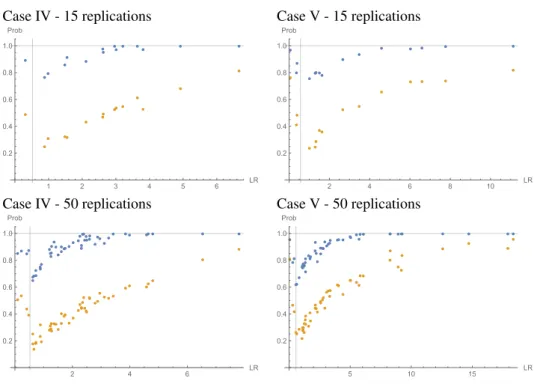
H0. In Figure 5, the blue dots are the upper RPs and the yellow dots are the lower RPs

evaluated for each simulated value of the likelihood ratio statistic.

In Figure 5 the vertical line marks the value of the exact quantile and the horizon-tal line marks the value 1. From Figure 5 we may observe the same features already described in Marques et al. (2018) for Case I, which are: the upper and lower RPs tend to increase and to be closer to each other when the simulated value of the likelihood

Figure 5: Lower (yellow dots) and upper (blue dots) reproducibility probabilities

Case IV - 15 replications Case V - 15 replications

                             1 2 3 4 5 6 LR 0.2 0.4 0.6 0.8 1.0 Prob                 _              2 4 6 8 10 LR 0.2 0.4 0.6 0.8 1.0 Prob

Case IV - 50 replications Case V - 50 replications

                                                                                                2 4 6 LR 0.2 0.4 0.6 0.8 1.0 Prob                                                                                                    5 10 15 LR 0.2 0.4 0.6 0.8 1.0 Prob

ratio statistic moves away from the quantile considered. When close to the quantile considered the lower RP is quite small which is a feature present in comparisons of two groups (Coolen and Bin Himd, 2014). As already mentioned the RP is a measure of how likely is to make the same decision if we repeat a test under the same circum-stances. When the lower RP is high it indicates that we may have a reasonable security that if the test were repeated we would end up with the same decision with regard to re-jection of the null hypothesis, thus ensuring the reproducibility of the test results. From Figure 5 we may observe that the lower RP only reaches values close, or equal, to 0.8 for quite distant values of the likelihood ratio statistics from the 0.1 quantile. This may suggest that in these cases the reproducibility of the test results is only guarantee for large values of the likelihood ratio.

4 Concluding remarks

In this paper we have studied the distribution of the likelihood ratio test statistic used to test between two Beta distributions. When two of the corresponding parameters of the two Beta distributions are equal and integers, representations of the exact distribution of the likelihood ratio statistic were obtained as transformations of a Gamma or of a GIG distribution. For the other three cases considered, near-exact or asymptotic

approximations, were developed. Using the exact distributions or the approximations developed, quantiles andp-values can be computed in a fast and precise way. This way, other more complex and time consuming methods, based on numerical methods or simulations, may be avoided. Similar results for the distribution of the likelihood ratio under the alternative hypothesis may be easily obtained using similar procedures. The power of the test increases with the sample size and when the values of the parameters are considerably different from the ones assumed in the null hypothesis, these are the already expected behaviours for likelihood ratio tests. The lower and upper RPs show that only for distant values of the likelihood ratio from the fixed quantile we may ensure the reproducibility of the test results. The authors aim, in the future, to address the case where the decision making involves more than two Beta distributions, and also tests between other types of distributions such as two Beta type II distributions or two Kumaraswamy distributions.

Acknowledgements

The authors would like thank the two Reviewers for their careful reading and construc-tive comments. This work was partially supported by the Fundac¸˜ao para a Ciˆencia e a Tecnologia (Portuguese Foundation for Science and Technology) through the project UID/MAT/00297/2013 (Centro de Matem´atica e Aplicac¸˜oes).

References

Arts G.R.J., Coolen F.P.A., van der Laan P., 2004. Nonparametric predictive inference in statistical process control. Quality Technology and Quantitative Management, 1, 201-216.

Coelho C.A., 1998. The Generalized Integer Gamma Distribution—A Basis for Distri-butions in Multivariate Statistics.Journal of Multivariate Analysis64, 86–102. Coelho C.A., 2004. The Generalized Near-Integer Gamma Distribution: A Basis for

‘Near-Exact’ Approximations to the Distribution of Statistics which are the Product of an Odd Number of Independent Beta Random Variables.Journal of Multivariate Analysis, 89, 191–218.

Coelho C.A. and Alberto R.P., 2012. On the Distribution of the Product of Independent Beta Random Variables Applications.Technical Report, CMA, 12.

Coelho C.A. and Marques F.J., 2012. Near-exact distributions for the likelihood ratio test statistic to test equality of several variance-covariance matrices in elliptically contoured distributions.Computational Statistics, 27, 627–659.

Coelho C.A., Arnold B.C. and Marques F.J., 2010. Near-exact distributions for certain likelihood ratio test statistics.Journal of Statistical Theory and Practice, 4, 711–725. Coolen F.P.A., Alqifari H.N., 2018. Nonparametric predictive inference for repro-ducibility of two basic tests based on order statistics.REVSTAT - Statistical Jour-nal, 16, 167-185

Coolen F.P.A., Bin Himd S., 2014. Nonparametric predictive inference for repro-ducibility of basic nonparametric tests. Journal of Statistical Theory and Practice, 8, 591-618.

Gil-Pelaez J., (1951). Note on the inversion theorem.Biometrika, 38, 481–482. Goodman S.N., (1992). A comment on replication, p-values and evidence.Statistics in

Medicine, 11, 875–879.

Griffiths, D. (1973). Maximum Likelihood Estimation for the Beta-Binomial Distribu-tion and an ApplicaDistribu-tion to the Household DistribuDistribu-tion of the Total Number of Cases of a Disease.Biometrics, 29, 637–648.

Gupta, A.K. and Nadarajah, S., (2004).Handbook of Beta Distribution and Its Appli-cations. Statistics: A Series of Textbooks and Monographs, Taylor & Francis. Hill B.M., 1968. Posterior distribution of percentiles: Bayes’ theorem for sampling

from a population.Journal of the American Statistical Association, 63, 677–691. Luke Y.L., (1969).The special functions and their approximations. Academic Press,

Inc., London.

Marques F.J., Coelho C.A. and de Carvalho M. 2015. On the distribution of linear combinations of independent Gumbel random variables.Stat Comput, 25, 683–701. Marques, F.J., Coelho, C.A. and Rodrigues, P.C., 2017. Testing the equality of several

linear regression models.Computational Statistics, in press

Marques F.J., Coolen F.P.A. and Coolen-Maturi T., 2018. Introducing nonparametric predictive inference methods for reproducibility of likelihood ratio tests.Journal of Statistical Theory and Practice, submitted for publication.

Pham, T.V., Piersma, S.R., Warmoes, M. and Jimenez, C.R. (2010). On the beta-binomial model for analysis of spectral count data in label-free tandem mass spectrometry-based proteomics.Bioinformatics, 26, 363-369.

Rachev, S.T., Hsu, J.S.J., Bagasheva, B.S. and Fabozzi, F.J. (2008).Bayesian Methods in Finance, Frank J. Fabozzi Series, John Wiley & Sons

Tricomi F.G. and Erd´elyi A., 1951. The asymptotic expansion of a ratio of Gamma functions.Pacific Journal of Mathematics1, 133–142.

Wiley, J.A., Martin, J.L., Herschkorn, S.J., and Bond, J. (2015). A New Extension of the Binomial Error Model for Responses to Items of Varying Difficulty in Educa-tional Testing and Attitude Surveys.PLoS ONE, 10, e0141981.

Wilks S.S., 1983. The Large-Sample Distribution of the Likelihood Ratio for Testing Composite Hypotheses.The Annals of Mathematical Statistics, 9, 60-62.