James Requeima12 Will Tebbutt12 Wessel Bruinsma12 Richard E. Turner1 1University of Cambridge and2Invenia Labs, Cambridge, UK
{jrr41, wct23, wpb23, ret26}@cam.ac.uk
Abstract
Multi-output regression models must exploit dependencies between outputs to maximise predictive performance. The application of Gaussian processes (GPs) to this setting typi-cally yields models that are computationally demanding and have limited representational power. We present the Gaussian Process Au-toregressive Regression (GPAR) model, a scal-able multi-output GP model that is scal-able to capture nonlinear, possibly input-varying, de-pendencies between outputs in a simple and tractable way: the product rule is used to decompose the joint distribution over the out-puts into a set of conditionals, each of which is modelled by a standard GP. GPAR’s effi-cacy is demonstrated on a variety of synthetic and real-world problems, outperforming exist-ing GP models and achievexist-ing state-of-the-art performance on established benchmarks.
1
Introduction
The Gaussian process (GP) probabilistic modelling framework provides a powerful and popular approach to nonlinear single-output regression (Rasmussen and Williams, 2006). The popularity of GP methods stems from their modularity, tractability, and interpretability: it is simple to construct rich, nonlinear models by com-positional covariance function design, which can then be evaluated in a principled way (e.g. via the marginal likelihood), before being interpreted in terms of their component parts. This leads to an attractive plug-and-play approach to modelling and understanding data, which is so robust that it can even be automated (Duvenaud et al., 2013; Sun et al., 2018).
Most regression problems, however, involve multiple outputs rather than a single one. When modelling such data, it is key to capture the dependencies between these outputs. For example, noise in the output space
Proceedings of the 22nd International Conference on
Ar-tificial Intelligence and Statistics (AISTATS) 2019, Naha, Okinawa, Japan. PMLR: Volume 89. Copyright 2019 by the author(s).
might be correlated, or, whilst one output might de-pend on the inputs in a complex (deterministic) way, it may depend quite simply on other output variables. In both cases multi-output GP models are required. There is a plethora of existing multi-output GP models that can capture linear correlations between output variables if these correlations are fixed across the in-put space (Goovaerts, 1997; Wackernagel, 2003; Teh and Seeger, 2005; Bonilla et al., 2008; Nguyen and Bonilla, 2014; Dai et al., 2017). However, one of the main reasons for the popularity of the GP approach is that a suite of different types of nonlinearinput depen-dencies can be modelled, and it is disappointing that this flexibility is not extended to interactions between theoutputs. There are some approaches that do allow limited modelling of nonlinear output dependencies (Wilson et al., 2012; Bruinsma, 2016) but this flexibil-ity comes from sacrificing tractabilflexibil-ity, with complex and computationally demanding approximate inference and learning schemes now required. This complexity significantly slows down model fitting, evaluation, and improvement work flow.
What is needed is a flexible and analytically tractable modelling approach to multi-output regression that supports plug-and-play modelling and model interpre-tation. The Gaussian Process Autoregressive Regres-sion (GPAR) model, introduced in Section 2, achieves these aims by taking an approach analogous to that em-ployed by the Neural Autoregressive Density Estimator (Larochelle and Murray, 2011) for density modelling. The product rule is used to decompose the distribu-tion of the outputs given the inputs into a set of one-dimensional conditional distributions. Critically, these distributions can be interpreted as a decoupled set of single-output regression problems, and learning and in-ference in GPAR therefore amount to a set of standard single-output GP regression tasks: training is closed form, fast, and amenable to standard scaling techniques. GPAR converts the modelling of output dependencies that are possibly nonlinear and input-dependent into a set of standard GP covariance function design problems, constructing expressive, jointly non-Gaussian models over the outputs. Importantly, we show how GPAR can capture nonlinear relationships between outputs as well as structured, input-dependent noise, simply through
CO2 C(t) =f2( , , t) Sea IceI(t) f1( , t) = TemperatureT(t)
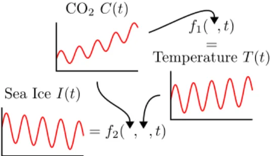
Figure 1: Cartoon motivating a factorisation for the joint distribution p(I(t), T(t), C(t))
kernel hyperparameter learning. We apply GPAR to a wide variety of multi-output regression problems, achieving state-of-the-art results on five benchmark tasks.
2
GPAR
Consider the problem of modelling the world’s average CO2 levelC(t), temperatureT(t), and Arctic sea ice
extent I(t)as a function of timet. By the greenhouse effect, one can imagine that the temperatureT(t)is a complicated, stochastic functionf1of CO2 and time: T(t) =f1(C(t), t). Similarly, one might hypothesise that the Arctic sea ice extentI(t)can be modelled as another complicated function f2 of temperature, CO2,
and time: I(t) = f2(T(t), C(t), t). These functional relationships are depicted in Figure 1 and motivate the following model where the conditionals model the postulated underlying functions f1 andf2:
p(I(t), T(t), C(t)) =p(C(t))p(T(t)|C(t)) | {z } modelsf1 p(I(t)|T(t), C(t)) | {z } modelsf2 .
More generally, consider the problem of modellingM
outputsy1:M(x) = (y1(x), . . . , yM(x))as a function of
the inputx. Applying the product rule yields1
p(y1:M(x)) (1) =p(y1(x))p(y2(x)|y1(x)) | {z } y2(x)as a random function ofy1(x) · · · p(yM(x)|y1:M−1(x)), | {z } yM(x)as a random function ofy1:M−1(x)
which states that y1(x), like CO2, is first generated
from x, according to some unknown, random function
f1; that y2(x), like temperature, is then generated fromy1(x)andx, according to some unknown, random functionf2; thaty3(x), like the Arctic sea ice extent, is then generated fromy2(x),y1(x), andx, according
1
This requires an ordering of the outputs; we will address this point in Section 2.
to some unknown, random functionf3;et cetera:
y1(x) =f1(x), f1∼p(f1),
y2(x) =f2(y1(x), x), f2∼p(f2), ..
.
yM(x) =fM(y1:M−1(x), x) fM ∼p(fM).
GPAR, introduced now, models these unknown func-tionsf1:M with Gaussian processes (GPs). Recall that
a GPf over an index setX defines a stochastic process, or process in short, where f(x1), . . . , f(xN)are jointly
Gaussian distributed for any x1, . . . , xN (Rasmussen
and Williams, 2006). Marginalising outf1:M, we find
that GPAR models the conditionals in Equation (1) with Gaussian processes:
ym|y1:m−1 (2)
∼ GP(0, km((y1:m−1(x), x),(y1:m−1(x0), x0))).
Although the conditionals in Equation (1) are Gaus-sian, the joint distribution p(y1:N)is not; moments of
the joint distribution over the outputs are generally intractable, but samples can be generated by sequen-tially sampling the conditionals. Figure 2b depicts the graphical model corresponding to GPAR. Crucially, the kernels(km) may specify nonlinear, input-dependent
relationships between outputs, which enables GPAR to model data where outputs inter-depend in complicated ways.
Returning to the climate modelling example, one might object that the temperature T(t) at time t does not just depend the CO2 level C(t) at time t, but
in-stead depends on the entire history of CO2 levelsC: T(t) =f1(C, t). Note: by writing C instead of C(t), we refer to the entire functionC, as opposed to just its value at t. Similarly, one might object that the Arctic sea ice extent I(t)at time tdoes not just depend on the temperature T(t) and CO2 level C(t) at time t,
but instead depends on the entire history of temper-atures T and CO2 levels C: T(t) =f2(T, C, t). This
kind of dependency structure, where outputym(x)now
depends on the entirety of all foregoing outputsy1:m
instead of just their value atx, motivates the following generalisation of GPAR in its form of Equation (2):
ym|y1:m−1∼GP(0, km((y1:m−1, x),(y1:m−1, x0))), (3) which we refer to as nonlocal GPAR, or non-instantaneous in the temporal setting. Clearly, GPAR is a special case of nonlocal GPAR. Figure 2a depicts the graphical model corresponding to nonlocal GPAR. Nonlocal GPAR will not be evaluated experimentally, but some theoretical properties will be described. Inference and learning in GPAR. Inference and learning in GPAR is simple. Let y(mn) =ym(x(n))
(a) f1 f2 f3 y1 y2 y3 (b) f1 f2 f3 y1(x) y2(x) y3(x) x
Figure 2: Graphical models corresponding to (a) non-local GPAR and (b) GPAR
outputs are observed at each input, we find
p(f1:M|(y (n) 1:M, x (n))N n=1) (4) = M Y m=1 p(fm| (y(mn)) N n=1 | {z } observations forfm ,(y1:(nm)−1, x (n))N n=1 | {z } input locations of observations ),
meaning that the posterior of fm is computed
sim-ply by conditioningfm on the observations for output
m located at the observations for the foregoing out-puts and the input, which again is a Gaussian process; thus, like the prior, the posterior predictive density also decomposes as a product of Gaussian condition-als. The evidencelogp((y(1:nM))
N
n=1|(x(n))Nn=1)
decom-poses similarly; as a consequence, the hyperparam-eters for fm can be learned simply by maximising
logp((y(mn))Nn=1|(y (n) 1:m−1, x
(n))N
n=1). In conclusion,
in-ference and learning in GPAR with M outputs comes down to inference and learning in M decoupled, one-dimensional GP regression problems. This shows that without approximations GPAR scales O(M N3), de-pending only linearly on the number of outputs M
rather than cubically, as is the case for general multi-output GPs, which scale O(M3N3).
Scaling GPAR. In these one-dimensional GP regres-sion problems, off-the-shelf GP scaling techniques may be applied to trivially scale GPAR to large data sets. Later we utilise the variational inducing point method by Titsias (2009), which is theoretically principled (Matthews et al., 2016) and empirically accurate (Bui et al., 2016b). This method requires a set of inducing inputs to be specified for each Gaussian process. For the first output y1 there is a single inputx, which is time. We use fixed (non-optimised) regularly spaced inducing inputs, as they are known to perform well for time series (Bui and Turner, 2014). The second and following outputsym, however, require inducing points
to be placed inxand y1, . . . , ym−1. Regular spacing
can be used again forx, but there are choices available for y1, . . . , ym−1. One approach would be to optimise
these inducing input locations, but instead we use the posterior predictive means of y1, . . . , ym−1 atx. This choice accelerates training and was found to yield good results.
Missing data. When there are missing outputs, the procedures for inference and learning described above remain valid as long as for every observationym(n)there
are also observations y(mn−)1:1. We call a data set satis-fying this propertyclosed downwards. If a data set is not closed downwards, data may be imputed, e.g. using the model’s posterior predictive mean, to ensure closed downwardness; inference and learning then, however, become approximate. The key conditional indepen-dence expressed by Figure 2b that results in simple inference and learning is the following:
Theorem 1. Let a set of observations D be closed downwards. Then yi ⊥ Di+1:M| D1:i, whereD1:i are
the observations for outputs 1, . . . , i and Di+1:M for
i+ 1, . . . , M.
Theorem 1 is proved in Appendix A from the sup-plementary material. Note that Theorem 1 holds for every graphical model of the form of Figure 2b, mean-ing that the decomposition into smean-ingle-output modellmean-ing problems holds for any choice of the conditionals in Equation (1), not just Gaussians.
Potential deficiencies of GPAR. GPAR has two apparent limitations. First, since the outputs from earlier dimensions are used as inputs to later dimen-sions, noisy outputs yield noisy inputs. One possible mitigating solution is to employ a denoising input transformation for the kernels, e.g. using the poste-rior predictive mean of the foregoing outputs as the input of the next covariance function. We shall refer to GPAR models employing this approach as D-GPAR. Second, one needs to choose an ordering of the outputs. Fortunately, often the data admits a natural ordering; for example, if the predictions concern a single output dimension, this should be placed last. Alternatively, if there is not a natural ordering, one can greedily opti-mise the evidence with respect to the ordering. This procedure considers 12M(M+ 1) configurations while an exhaustive search would consider all M! possible configurations: the best first output is selected out of all M choices, which is then fixed; then, the best second output is selected out of the remainingM−1 choices, which is then fixed; et cetera. These methods are examined in Section 6.
3
GPAR and Multi-Output GPs
The choice of kernelsk1:M forf1:M is crucial to GPAR,
as they determine the types of relationships between inputs and outputs that can be learned. Particular choices fork1:M turn out to yield models closely related
to existing work. These connections are made rigorous by the nonlinear and linear equivalent model discussed in Appendix B from the supplementary material. We
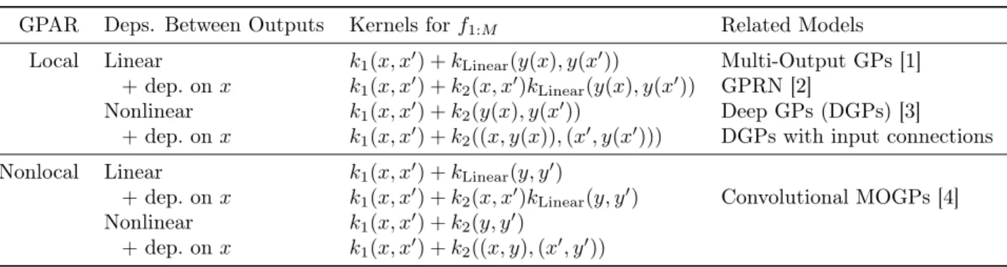
summarise the results here; see also Table 1.
Ifkmdepends linearly on the foregoing outputsy1:m−1 at particularx, then a joint Gaussian distribution over the outputs is induced in the form of a multi-output GP model (Goovaerts, 1997; Stein, 1999; Wackernagel, 2003; Teh and Seeger, 2005; Bonilla et al., 2008; Nguyen and Bonilla, 2014) where latent processes are mixed together according to a matrix, called the mixing ma-trix, that islower-triangular (Appendix B). One may let the dependency of km on y1:m−1 vary with x, in which case the mixing matrix varies withx, meaning that correlations between outputs vary with x. This yields an instance of the Gaussian Process Regression Network (GPRN) (Wilson et al., 2012) where inference is fast and closed form. One may even let km
de-pend nonlinearly ony1:m−1, which yields a particularly
structured deep Gaussian process (DGP) (Damianou, 2014; Bui et al., 2016a), potentially with skip connec-tions from the inputs (Appendix B). Note that GPAR may be interpreted as a conventional DGP where the hidden layers are directly observed and correspond to successive outputs; this connection could potentially be leveraged to bring machinery developed for DGPs to GPAR, e.g. to deal with arbitrarily missing data. One can further letkmdepend on theentirety of the
foregoing outputsy1:m−1, yielding instances of nonlocal
GPAR. An example of a nonlocal linear kernel is
k((y, x),(y0, x0)) =Z a(x −z, x0
−z0)y(z)y0(z0) dzdz0.
The nonlocal linear kernel again induces a jointly Gaus-sian distribution over the outputs in the form of a convolutional multi-output GP model (Álvarez et al., 2009; Álvarez and Lawrence, 2009; Bruinsma, 2016) where latent processes are convolved together accord-ing to a matrix-valued function, called theconvolution matrix, that islower-triangular (Appendix B). Again, one may let the dependency of km on the entirety of
y1:m−1 vary withx, in which case the convolution ma-trix varies withx, or even letkm depend nonlinearly
on the entirety of y1:m−1; an example of a nonlocal
nonlinear kernel is k(y, y0) =σ2exp − Z 1 2`(z)(y(z)−y 0(z))2dz .
Henceforth, we shall refer to GPAR with linear de-pendencies between outputs as GPAR-L, GPAR with nonlinear dependencies between outputs as GPAR-NL, and a combination of the two as GPAR-L-NL.
4
Further Related Work
The Gaussian Process Network (Friedman and Nach-man, 2000) is similar to GPAR, but was instead devel-oped to identify causal dependencies between variables
in a probabilistic graphical models context rather than multi-output regression. The work by Yuan (2011) also discusses a model similar to GPAR, but specifies a different generative procedure for the outputs. The multi-fidelity modelling literature is closely related to multi-output modelling. Whereas in a multi-output regression task we predict all outputs, multi-fidelity modelling is concerned with predicting a particular high-fidelity function, incorporating information from observations from various levels of fidelity. The idea of iteratively conditioning on lower fidelity models in the construction of higher fidelity ones is a well-used strategy (Kennedy and O’Hagan, 2000; Le Gratiet and Garnier, 2014). The model presented by Perdikaris et al. (2017) is nearly identical to GPAR applied in the multi-fidelity framework, but applications outside this setting have not been considered.
Moreover, GPAR follows a long line of work on the family of fully visible Bayesian networks (Frey et al., 1996; Bengio and Bengio, 2000) that decompose the distribution over the observations according to the product rule (Equation (1)) and model the resulting one dimensional conditionals. A number of approaches use neural networks for this purpose (Neal, 1992; Frey et al., 1996; Larochelle and Murray, 2011; Theis and Bethge, 2015; van den Oord et al., 2016). In particular, if the observations are real-valued, a standard archi-tecture lets the conditionals be Gaussian with means encoded by neural networks and fixed variances. Under broad conditions, if these neural networks are replaced by Bayesian neural networks with independent Gaus-sian priors over the weights, we recover GPAR as the width of the hidden layers goes to infinity (Neal, 1996; Matthews et al., 2018).
5
Synthetic Data Experiments
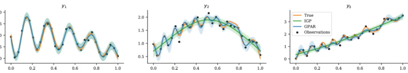
GPAR is well suited for problems where there is a strong functional relationship between outputs and for problems where observation noise is richly structured and input dependent. In this section we demonstrate GPAR’s ability to model both types of phenomena. First, we test the ability to leverage strong functional relationships between the outputs. Consider three out-puts y1,y2, andy3, inter-depending nonlinearly:
y1(x) =−sin(10π(x+ 1))/(2x+ 1)−x4+ 1, y2(x) = cos2(y1(x)) + sin(3x) + 2, y3(x) =y2(x)y2 1(x) + 3x+3,
where1, 2, 3i.i.d.∼ N(0,0.05). By substitutingy1and
y2into y3, we see thaty3 can be expressed directly in terms ofx, but via a complex function. The dependence ofy3ony1,y2, however, is much simpler. Therefore, as GPAR can exploit direct dependencies betweeny1:2and
GPAR Deps. Between Outputs Kernels forf1:M Related Models
Local Linear k1(x, x0) +kLinear(y(x), y(x0)) Multi-Output GPs [1]
+dep. onx k1(x, x0) +k2(x, x0)kLinear(y(x), y(x0)) GPRN [2]
Nonlinear k1(x, x0) +k2(y(x), y(x0)) Deep GPs (DGPs) [3]
+dep. onx k1(x, x0) +k2((x, y(x)),(x0, y(x0))) DGPs with input connections
Nonlocal Linear k1(x, x0) +kLinear(y, y0)
+dep. onx k1(x, x0) +k2(x, x0)kLinear(y, y0) Convolutional MOGPs [4]
Nonlinear k1(x, x0) +k2(y, y0)
+dep. onx k1(x, x0) +k2((x, y),(x0, y0))
Table 1: Classification of kernelsk1:M forf1:M, the resulting dependencies between outputs, and related models.
HerekLinear refers to a linear kernel andk1andk2to an exponentiated quadratic (EQ) or rational quadratic (RQ) kernel (Rasmussen and Williams, 2006). [1]: Goovaerts (1997); Stein (1999); Wackernagel (2003); Teh and Seeger (2005); Bonilla et al. (2008); Osborne et al. (2008); Nguyen and Bonilla (2014). [2]: Wilson et al. (2012). [3]: Damianou (2014); Bui et al. (2016a). [4]: Álvarez et al. (2009); Álvarez and Lawrence (2009); Bruinsma (2016).
y3, it should be presented with a much simplified task as compared to predicting y3 fromxdirectly. Figure 3 shows plots of independent GPs (IGPs) and GPAR fit to30data points from y1,y2 andy3. Indeed observe that GPAR is able to learny2’s dependence ony1, and
y3’s dependence ony1andy2, whereas the independent GPs struggle with the complicated structure.
Second, we test GPAR’s ability to capture non-Gaussian and input-dependent noise. Consider the fol-lowing three schemes in which two outputs are observed under various noise conditions: y1(x) =f1(x) +1 and
(1): y2(x) =f2(x) + sin2(2πx)
1+ cos2(2πx)2, (2): y2(x) =f2(x) + sin(π1) +2,
(3): y2(x) =f2(x) + sin(πx)1+2,
where1, 2 i.i.d.∼ N(0,0.1), andf1 andf2 are compli-cated, nonlinear functions.2 All three schemes have
i.i.d. homoscedastic Gaussian noise in y1. The noise in y2, however, depends on that in y1 and can be heteroscadastic. The task for GPAR is to learn the scheme’s noise structure. Figure 4 visualises the noise correlations induced by the schemes and the noise struc-tures learned by GPAR. Observe that GPAR is able to learn the various noise structures.
6
Real-World Data Experiments
In this section we evaluate GPAR’s performance and compare to other models on four standard data sets commonly used to evaluate multi-output models. We also consider a recently-introduced data set in the field of Bayesian optimisation, which is a downstream ap-plication area that could benefit from GPAR. Table 2 lists the models against which we compare GPAR. We
2The functions given byf1(x) =−sin(10π(x+ 1))/(2x+ 1)−x4 and f2(x) = 1 5e 2x(θ1cos(θ2πx) +θ3cos(θ4πx)) + √ 2x. Acronym Model IGP Independent GPs CK Cokriging
ICM Intrinstic Coregionalisation Model [1] SLFM Semi-Parametric Latent Factor Model [2] CGP Collaborative Multi-Output GPs [3] CMOGP Convolved Multi-Output GP Model [4] GPRN GP Regression Network [5]
Table 2: Models against which GPAR is compared. [1]: Goovaerts (1997); Stein (1999); Wackernagel (2003). [2]: Teh and Seeger (2005). [3]: Nguyen and Bonilla (2014). [4]: Álvarez and Lawrence (2011); Álvarez et al. (2010). [5]: Wilson et al. (2012).
always compare against IGP and CK, ICM, SLFM, and CGP, and compare against CMOGP and GPRN if results for the considered task are available. Since CK and ICM are much simplified versions of SLFM (Álvarez et al., 2010; Goovaerts, 1997) and CGP is an approximation to SLFM, we sometimes omit results for CK, ICM, and CGP. Implementations can be found athttps://github.com/wesselb/gpar(Python) and https://github.com/willtebbutt/GPAR.jl (Julia). Experimental details can be found in Appendix D from the supplementary material.
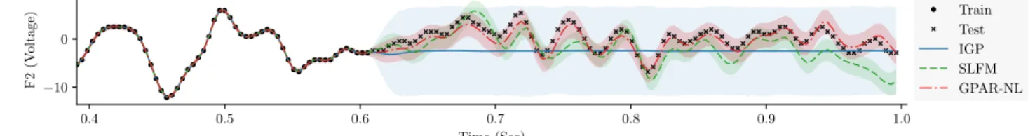
Electroencephalogram (EEG) data set.3 This data set consists of 256 voltage measurements from 7 electrodes placed on a subject’s scalp whilst the subject is shown a certain image; Zhang et al. (1995) describe the data collection process in detail. In par-ticular, we use frontal electrodes FZ and F1–F6 from the first trial on control subject 337. The task is to predict the last 100 samples for electrodes FZ, F1, and F2, given that the first 156 samples of FZ, F1, and F2
3
The EEG data set can be downloaded athttps:// archive.ics.uci.edu/ml/datasets/eeg+database.
Figure 3: Synthetic data set with complex output dependencies: GPAR vs independent GPs (IGP) predictions.
Figure 4: Correlation between the sample residues (deviation from the mean) fory1 andy2. Left, middle, and right plots correspond to schemes (1), (2) and (3) respectively. Samples are coloured according to input valuex; that is, all samples for a particular xhave the same colour. If the colour pattern is preserved, then GPAR has successfully captured how the noise in y1 correlates to that in y2.
Model SMSE MLL TT
IGP 1.75 2.60 2 sec SLFM 1.06 4.00 11 min GPAR-NL 0.26 1.63 5 sec
Table 3: Results for the EEG data set for IGP, the SLFM with four latent dimensions, and GPAR.
and the whole signals of F3–F6 are observed. Perfor-mance is measured with the standardised mean squared error (SMSE), mean log loss (MLL) (Rasmussen and Williams, 2006), and training time (TT). Figure 5 visualises predictions for electrode F2, and Table 3 quantifies the results. We observe that GPAR-NL out-performs independent in terms of SMSE and MLL; note that independent GPs completely fail to provide an informative prediction. Furthermore, independent GPs were trained in two seconds, and GPAR-NL took only three more seconds; in comparison, training SLFM took 11 minutes.
Jura data set.4 This data set comprises metal
con-centration measurements collected from the topsoil in a 14.5 km2 region of the Swiss Jura. We follow the
ex-4
The data can be downloaded at https: //sites.google.com/site/goovaertspierre/
pierregoovaertswebsite/download/.
Model IGP CK† ICM SLFM CMOGP†
MAE 0.5739 0.51 0.4601 0.4606 0.4552 MAE∗ 0.5753 0.4114 0.4145
Model GPRN† GPAR-NL D-GPAR-NL MAE 0.4525 0.4324 0.4114
MAE∗ 0.4040 0.4168 0.3996
Table 4: Results for the Jura data set for IGP, cok-riging (CK) and ICM with two latent dimensions, the SLFM with two latent dimensions, CMOGP, GPRN, and GPAR. ∗ Results are obtained by first log-transforming the data, then performing prediction, and finally transforming the predictions back to the original domain. † Results from Wilson (2014).
perimental protocol by Goovaerts (1997) also followed by Álvarez and Lawrence (2011): The training data comprises 259 data points distributed spatially with three output variables—nickel, zinc, and cadmium— and 100 additional data points for which only two of the three outputs—nickel and zinc—are observed. The task is to predict cadmium at the locations of those 100 additional data. Performance is evaluated with the mean absolute error (MAE).
Table 4 shows the results. The comparatively poor performance of independent GPs highlights the impor-tance of exploiting correlations between the mineral concentrations. Furthermore, Table 4 shows that D-GPAR-NL significantly outperforms the other models, achieving a new state-of-the-art.
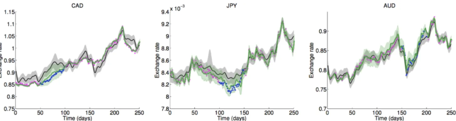
Exchange rates data set.5 This data set consists
of the daily exchange rate w.r.t. USD of the top ten international currencies (CAD, EUR, JPY, GBP, CHF, AUD, HKD, NZD, KRW, and MXN) and three precious metals (gold, silver, and platinum) in the year 2007. The task is to predict CAD on days 50–100, JPY on days 100–150, and AUD on days 150–200, given that CAD is observed on days 1–49 and 101–251, JPY on days 1–99 and 151–251, and AUD on days 1–149 and 201–251; and that all other currencies are observed throughout the whole year. Performance is measured
5
The exchange rates data set can be downloaded at
0.4 0.5 0.6 0.7 0.8 0.9 1.0 Time (Sec) −10 0 F2 (V oltage) Train Test IGP SLFM GPAR-NL
Figure 5: Predictions for electrode F2 from the EEG data set
Model IGP∗ CMOGP∗ CGP∗ GPAR-L-NL SMSE 0.5996 0.2427 0.2125 0.0302
Table 5: Experimental results for the exchange rates data set for IGP, CMOGP, CGP, and GPAR. ∗These numbers are taken from Nguyen and Bonilla (2014).
with the SMSE.
Figure 6 visualises GPAR’s prediction for data set, and Table 5 quantifies the result. We greedily optimise the evidence w.r.t. the ordering of the outputs to determine an ordering, and we impute missing data to ensure closed downwardness of the data. Observe that GPAR significantly outperforms all other models.
Tidal height, wind speed, and air temperature data set.6 This data set was collected at 5 minute in-tervals by four weather stations: Bramblemet, Camber-met, ChiCamber-met, and SotonCamber-met, all located in Southamp-ton, UK. The task is to predict the air temperature measured by Cambermet and Chimet from all other signals. Performance is measured with the SMSE. This experiment serves two purposes. First, it demonstrates that it is simple to scale GPAR to large data sets using off-the-shelf inducing point techniques for single-output GP regression. Second, it shows that scaling to large data sets enables GPAR to better learn dependencies between outputs, which, importantly, can significantly improve predictions in regions where outputs are par-tially observed. We utilise the variational inducing point method by Titsias (2009) as discussed in Sec-tion 2, with 10 inducing points per day. This data set is not closed downwards, so we use mean imputation when training. We use D-GPAR-L and set the tempo-ral kernel to be a simple EQ, meaning that the model cannot make long-range predictions, but instead must exploit correlations between outputs.
Nguyen and Bonilla (2014) consider from this data set 5 days in July 2013, and predict short periods of the air temperature measured by Cambermet and Chimet using all other signals. We followed their setup and predicted the same test set, but instead trained on
6
The data can be downloaded at http://www. bramblemet.co.uk, http://cambermet.co.uk, http:// www.chimet.co.uk, andhttp://sotonmet.co.uk.
the whole of July. Even though the additional ob-servations do not temporally correlate with the test periods at all, they enable GPAR to better learn the relationships between the outputs, which, unsurpris-ingly, significantly improved the predictions: using the whole of July, GPAR achieves SMSE0.056, compared to their SMSE 0.107.
The test set used by Nguyen and Bonilla (2014) is rather small, yielding high-variance test results. We therefore do not pursue further comparisons on their train–test split, but instead consider a bigger, more challenging setup: using as training data 10 days (days [10,20), roughly 30 k points), 15 days (days [18,23), roughly 47 k points), and the whole of July (roughly 98 k points), make predictions of 4 day periods of the air temperature measured by Cambermet and Chimet. Figure 7 visualises the test periods and GPAR’s pre-dictions for it. Despite the additional observations not correlating with the test periods, we observe clear, though dimishining, improvements in the predictions as the training data is increased.
MLP validation error data set. The final data set is the validation error of a multi-layer perceptron (MLP) on the MNIST data, trained using categorical cross-entropy, and set as a function of six hyperpa-rameters: the number of hidden layers, the number of neurons per hidden layer, the dropout rate, the learning rate to use with the ADAM optimizer, the L1 weight penalty, and theL2weight penalty. This exper-iment was implemented using code made available by Hernández-Lobato (2016). An improved model for the objective surface could translate directly into improved performance in Bayesian optimisation (Snoek et al., 2012), as this would enable a more informed search of the hyperparameter space.
To generate a data set, we sample 291 sets of hyperpa-rameters randomly from a rectilinear grid and train the MLP for 21 epochs under each set of hyperparameters, recording the validation performance after 1, 5, 11, 16, and 21 epochs. We construct a training set of 175 of these hyperparameter settings and, crucially, discard roughly 30% of the validation performance results at 5 epochs at random, and again discard roughly 30% of those results at 11 epochs, and so forth. The resulting data set has 175 labels after 1 epoch, 124 after 5, 88
Figure 6: Visualisation of the exchange rates data set and CGP’s (black) and GPAR’s (green) predictions for it. GPAR’s predictions are overlayed on the original figure by Nguyen and Bonilla (2014).
Figure 7: Visualisation of the air temperature data set and GPAR’s prediction for it. Black circles indicate the locations of the inducing points.
1 6 11 16 21
Epoch at Which to the Predict Validation Error 0.4 0.6 0.8 1.0 SMSE of V alidation Error Prediction IGP SLFM GPAR-L-NL
Figure 8: Results for the machine learning data set for a GP, the SLFM with two latent dimensions, and GPAR
after 11, 64 after 15 and 44 after 21, simulating the partial completion of the majority of runs. Importantly, a Bayesian Optimisation system typically exploits only completed training runs to inform the objective surface, whereas GPAR can also exploit partially complete runs. The results presented in Figure 8 show the SMSE in predicting validation performance at each epoch using GPAR, the SLFM, and independent GPs on the test set, averaged over 10 seed for the pseudo-random num-ber generator used to select which outputs from the training set to discard. GPs trained independently to predict performance after a particular number of epochs perform worse than the SLFM and GPAR, which both
have learned to exploit the extra information available. In turn, GPAR noticeably outperforms the SLFM.
7
Conclusion and Future Work
This paper introduced GPAR: a flexible, fast, tractable, and interpretable approach to multi-output GP re-gression. GPAR can model (1) nonlinear relation-ships between outputs and (2) complex output noise. GPAR can scale to large data sets by trivially lever-aging scaling techniques for one-dimensional GP re-gression (Titsias, 2009). In effect, GPAR transforms high-dimensional data modelling problems into set of single-output modelling problems, which are the bread and butter of the GP approach. GPAR was rigorously tested on a variety of synthetic and real-world prob-lems, consistently outperforming existing GP models for multi-output regression. An exciting future appli-cation of GPAR is to use compositional kernel search (Lloyd et al., 2014) to automatically learn and explain dependencies between outputs and inputs. Further insights into structure of the data could be gained by decomposing GPAR’s posterior over additive kernel components (Duvenaud, 2014). These two approaches could be developed into a useful tool for automatic structure discovery. Two further exciting future ap-plications of GPAR are modelling of environmental phenomena and improving data efficiency of existing Bayesian optimisation tools (Snoek et al., 2012).
Acknowledgements
Richard E. Turner is supported by Google as well as EPSRC grants EP/M0269571 and EP/L000776/1.
References
Álvarez, M. and Lawrence, N. D. (2009). Sparse con-volved gaussian processes for multi-output regression. Advances in Neural Information Processing Systems, 21:57–64.
Álvarez, M. A. and Lawrence, N. D. (2011). Computa-tionally efficient convolved multiple output Gaussian processes. Journal of Machine Learning Research, 12:1459–1500.
Álvarez, M. A., Luengo, D., and Lawrence, N. D. (2009). Latent force models.Artificial Intelligence and Statis-tics, 5:9–16.
Álvarez, M. A., Luengo, D., Titsias, M. K., and Lawrence, N. D. (2010). Efficient multioutput Gaus-sian processes through variational inducing kernels. Journal of Machine Learning Research: Workshop and Conference Proceedings, 9:25–32.
Bengio, Y. and Bengio, S. (2000). Modeling high-dimensional discrete data with multi-layer neural networks. InAdvances in Neural Information Pro-cessing Systems, pages 400–406.
Bonilla, E. V., Chai, K. M., and Williams, C. K. I. (2008). Multi-task Gaussian process prediction. Ad-vances in Neural Information Processing Systems, 20:153–160.
Bruinsma, W. P. (2016). The generalised gaussian convolution process model. MPhil thesis, Department of Engineering, University of Cambridge.
Bui, T. D., Lobato, D., Li, Y., Hernández-Lobato, J. M., and Turner, R. E. (2016a). Deep gaussian processes for regression using approxi-mate expectation propagation. arXiv preprint arXiv:1602.04133.
Bui, T. D. and Turner, R. E. (2014). Tree-structured Gaussian process approximations. Advances in Neu-ral Information Processing Systems, 27:2213–2221. Bui, T. D., Yan, J., and Turner, R. E. (2016b). A
unifying framework for gaussian process pseudo-point approximations using power expectation propagation. arXiv preprint arXiv:1605.07066.
Dai, Z., Álvarez, M. A., and Lawrence, N. D. (2017). Efficient modeling of latent information in supervised learning using Gaussian processes. arXiv preprint arXiv:1705.09862.
Damianou, A. (2014). Deep Gaussian Processes and Variational Propagation of Uncertainty. PhD thesis, Department of Neuroscience, University of Sheffield.
Duvenaud, D. (2014). Automatic Model Construction with Gaussian Processes. PhD thesis, Computational and Biological Learning Laboratory, University of Cambridge.
Duvenaud, D., Lloyd, J. R., Grosse, R., Tenenbaum, J. B., and Ghahramani, Z. (2013). Structure discov-ery in nonparametric regression through composi-tional kernel search. In International Conference on Machine Learning.
Frey, B. J., Hinton, G. E., and Dayan, P. (1996). Does the wake-sleep algorithm produce good density esti-mators? In Advances in neural information process-ing systems, pages 661–667.
Friedman, N. and Nachman, I. (2000). Gaussian process networks. In Uncertainty in Artificial Intelligence, pages 211–219. Morgan Kaufmann Publishers Inc. Goovaerts, P. (1997). Geostatistics for Natural
Re-sources Evaluation. Oxford University Press, 1 edi-tion.
Hernández-Lobato, J. M. (2016). Neural networks with optimal accuracy and speed in their predictions. Kennedy, M. C. and O’Hagan, A. (2000). Predicting
the output from a complex computer code when fast approximations are available. Biometrika, 87(1):1– 13.
Larochelle, H. and Murray, I. (2011). The neural au-toregressive distribution estimator. In AISTATS, volume 1, page 2.
Le Gratiet, L. and Garnier, J. (2014). Recursive co-kriging model for design of computer experiments with multiple levels of fidelity. International Journal for Uncertainty Quantification, 4(5).
Lloyd, J. R., Duvenaud, D., Grosse, R., Tenenbaum, J. B., and Ghahramani, Z. (2014). Automatic con-struction and natural-language description of non-parametric regression models. InAssociation for the Advancement of Artificial Intelligence (AAAI). Matthews, A. G. D. G., Hensman, J., Turner, R. E.,
and Ghahramani, Z. (2016). On sparse variational methods and the kullback-leibler divergence be-tween stochastic processes. Artificial Intelligence and Statistics, 19.
Matthews, A. G. d. G., Rowland, M., Hron, J., Turner, R. E., and Ghahramani, Z. (2018). Gaussian pro-cess behaviour in wide deep neural networks. arXiv preprint arXiv:1804.11271.
Neal, R. M. (1992). Connectionist learning of belief networks. Artificial intelligence, 56(1):71–113. Neal, R. M. (1996). Bayesian learning for neural
net-works, volume 118. Springer Science & Business Media.
Nguyen, T. V. and Bonilla, E. V. (2014). Collaborative multi-output Gaussian processes. Conference on Uncertainty in Artificial Intelligence, 30.
Osborne, M. A., Roberts, S. J., Rogers, A., Ramchurn, S. D., and Jennings, N. R. (2008). Towards real-time information processing of sensor network data us-ing computationally efficient multi-output Gaussian processes. In Proceedings of the 7th International Conference on Information Processing in Sensor Net-works, IPSN ’08, pages 109–120. IEEE Computer Society.
Perdikaris, P., Raissi, M., Damianou, A., Lawrence, N. D., and Karniadakis, G. E. (2017). Nonlinear information fusion algorithms for data-efficient multi-fidelity modelling. Proceedings of the Royal Society A: Mathematical, Physical and Engineering Science, 473.
Rasmussen, C. E. and Williams, C. K. I. (2006). Gaus-sian Processes for Machine Learning. MIT Press. Snoek, J., Larochelle, H., and Adams, R. P. (2012).
Practical bayesian optimization of machine learn-ing algorithms. In Advances in Neural Information Processing Systems, pages 2951–2959.
Stein, M. (1999). Interpolation of Spatial Data. Springer-Verlag New York, 1 edition.
Sun, S., Zhang, G., Wang, C., Zeng, W., Li, J., and Grosse, R. (2018). Differentiable compositional ker-nel learning for gaussian processes. International Conference on Machine Learning, 35.
Teh, Y. W. and Seeger, M. (2005). Semiparametric latent factor models. International Workshop on Artificial Intelligence and Statistics, 10.
Theis, L. and Bethge, M. (2015). Generative image modeling using spatial lstms. In Advances in Neural Information Processing Systems, pages 1927–1935. Titsias, M. K. (2009). Variational learning of inducing
variables in sparse Gaussian processes. Artificial Intelligence and Statistics, 12:567–574.
van den Oord, A., Kalchbrenner, N., Espeholt, L., Vinyals, O., Graves, A., et al. (2016). Conditional image generation with pixelcnn decoders. In Ad-vances in Neural Information Processing Systems, pages 4790–4798.
Wackernagel, H. (2003). Multivariate Geostatistics. Springer-Verlag Berlin Heidelberg, 3 edition. Wilson, A. G. (2014). Covariance Kernels for Fast
Au-tomatic Pattern Discovery and Extrapolation With Gaussian Processes. PhD thesis, University of Cam-bridge.
Wilson, A. G., Knowles, D. A., and Ghahramani, Z. (2012). Gaussian process regression networks. Inter-national Conference on Machine Learning, 29.
Yuan, C. (2011). Conditional multi-output regression. In International Joint Conference on Neural Net-works, pages 189–196. IEEE.
Zhang, X., Begleiter, H., Porjesz, B., Wang, W., and Litke, A. (1995). Event related potentials during object recognition tasks. Brain Research Bulletin, 38(6):531–538.