Asymmetric loss utility: an analysis of decision under risk

Full text

(1)Asymmetric loss utility: an analysis of decision under risk Alex Strashny University of California, Irvine [email protected] May 26, 2004 Original: November 10, 2003. Abstract This paper develops a utility model for evaluating lotteries. In estimating utility, risk averse people use an asymmetric loss function. Expected utility is seen as a special case that is a good approximation of the general case in some cases. The model resolves several paradoxes and makes easily falsifiable predictions. When used in hypothesis testing, the model allows researchers to directly specify their attitudes toward risk. The model is advantageous for two reasons. First, it is based on established principles of probability; second, it resolves several wellknown paradoxes.. Keywords: choice under uncertainty, non-expected utility theory, risk aversion, Allais paradox, Ellsberg paradox, St. Petersburg paradox, Equity Premium Puzzle, decision theory. 1.

(2) 1. Introduction. Suppose a lottery L has M outcomes numbered m = 1, 2, . . . M, P and outcome bm occurs with probability pm , pm = 1. The. elementary utility of an outcome b is u(b). The most common way of calculating the utility of the lottery is using the expected utility theory, which states that the utility of a lottery is the expected elementary utility:. UE (L) = Eu =. M X. pm u(bm ).. (1). m=1. There are several problems with expected utility. Aside from the theoretical problems, there are more practical ones as well. For example, expected utility fails to explain several well known paradoxes, such as the Allais paradox, Ellsberg paradox, St. Petersburg paradox, and the Equity Premium Puzzle. In this paper, I take a different approach. The utility of a lottery, after the lottery’s outcome is known, is the elementary utility of the outcome. That is, if we know that the lottery’s outcome is bm , then U(L) = u(bm ). Before the outcome is known, the utility of a lottery is a random variable. What people mean when they refer to the utility of a lottery is actually a point 2.

(3) estimate of the random variable. This approach has two advantages. First, it is based on established principles of probability; second, it resolves several well-known paradoxes. Expected value is the optimal estimator under quadratic loss, which is a symmetric loss function. In my view, a symmetric loss function reflects risk neutrality. A risk averse individual uses an asymmetric loss function in which higher loss comes from overestimating utility. This causes his estimates of utility to be, in general, less than expected utility. In section 2, I describe the model. In section 3, I look at several well-known paradoxes. Finally, in section 4, I discuss the model in the context of hypothesis testing.. 2. Utility. Suppose a person plans to play some lottery a total of n times, and that outcome bm occurs xm times. The total utility from all n games is:. nŨ(L) =. M X. xm u (bm ) .. (2). m=1. Define the utility of the lottery as the average per-game utility 3.

(4) after n games. That is,. Ũ(L) =. M ³ X xm ´. n. m=1. u (bm ) .. (3). In the above equations, since counts xm are random variables, so is Ũ(L). When evaluating lotteries, people estimate the utilities of those lotteries. I denote the random variable by Ũ (L) and its estimate by by U(L). Risk neutral individuals care about overestimating and underestimating utility equally: they have a symmetric loss function. For instance, people who minimize expected quadratic loss, estimate the utility of a lottery by the expected value over elementary utilities. Risk averse individuals would rather underestimate utility than overestimate it: they have an asymmetric loss function in which overestimation is penalized more than underestimation. If the probabilities pm are known, then counts {xm } have the Multinomial distribution as follows:. {xm } |n, {pm } ∼ Mult (n, {pm }) .. (4). In the case when there are M = 2 possible outcomes, this reduces to the Binomial distribution.. 4.

(5) Sometimes, the probabilities pm themselves are unknown. This is not a problem if their distribution is known. Suppose the probabilities {pm } are a priori Dirichlet distributed with parameter vector {αm }. (In case M = 2, this is the same as the Beta distribution.) We observe k outcomes. In these observations, outcome bm occurs ym times. Then, the posterior distribution of the probabilities is Dirichlet:. {pm } | {ym } ∼ D ({αm + ym }) .. (5). From this, when probabilities pm are not known, counts xm have the Multinomial-Dirichlet distribution. Note that, if the probabilities pm are known, as the number of games n approaches infinity, by the frequentist definition of ¡ ¢ probability, the weights nx approach the probabilities p. Thus, lim Ũ (L) = UE (L) .. n→∞. (6). So, any reasonable estimator of Ũ(L) must also approach expected utility UE (L). In other words, expected utility theory can be thought of in two ways. First, it accurately reflects preferences of risk neutral individuals with symmetric quadratic. 5.

(6) loss. Second, it is a limiting case when the number of games n approaches infinity and there is no uncertainty. 2.1. Loss function. A loss function C(Ũ, U) expresses the loss that an individual experiences from estimating random utility Ũ by some estimate U. To find the optimal estimate, the individual minimizes expected loss. If f (Ũ) is the probability mass function of Ũ, then. h ³ í ´ X ³ E C Ũ, U = C Ũ, U f (Ũ). (7). Ũ. h ³ í U = arg min E C Ũ, U U. (8). Each individual may have his own unique loss function C (·, ·). When discussing attitudes toward risk, we are interested in how loss function penalizes overestimation as opposed to underestimation of utility. Let ∆ > 0 be some constant. If a person is indifferent between overestimating and underestimating utility, that is, if C(U, U + ∆) = C(U, U − ∆), I call him risk neutral. If a person is more afraid to overestimate utility, that is, if C(U, U + ∆) > C(U, U − ∆), then he is risk 6.

(7) averse. Finally, if he is more afraid of underestimating utility, C(U, U + ∆) < C(U, U − ∆), then he is risk loving. To perform calculations, we need to define a specific loss function. In this paper, I use the following asymmetric loss: ⎧ ³ á ³ ´ ⎨ Ũ − U if Ũ ≥ U ¯ ¯a , Ca Ũ, U = ⎩ c ¯¯Ũ − U ¯¯ if Ũ < U a. (9). where a ≥ 0 and ca ≥ 0 are constants. ca > 1 reflects risk aversion, while ca = 1 reflects risk neutrality. When a → 0 and c0 = 1, the loss function is called the all-or-none loss; when a = 1, it is the asymmetric linear loss; when a = 2, this is the asymmetric quadratic loss; when a = 2 and c2 = 1, it is the usual quadratic loss. Because a defines the general shape of the loss function, I call it the type of loss; because ca defines the degree of asymmetry, I call it risk aversion. For linear (type 1) loss, there is an analytical solution for the best estimator U. Define q = (1 + c1 )−1 ; the best estimator under type 1 loss is the q-th quantile of Ũ. Thus, for symmetric linear loss, the best estimator is the median of Ũ. If the loss is symmetric quadratic (a = 2, c2 = 1), then the best estimator 7.

(8) is the expected value of Ũ. For arbitrary values of a and ca , however, I don’t know of a general analytical solution, but find best estimates numerically. The type of loss and risk aversion that people commonly have need to be determined experimentally. In this paper, I concentrate on three types of loss. I use the linear (type 1) loss because there is an analytical solution for the best estimator under this loss. A problem with this loss is that for discrete random variables, the estimator of utility U (L) is not a continuous function of risk aversion c1 . Quadratic (type 2) loss is also attractive, because symmetric quadratic loss is used so often. But because there is no analytical solution for it, I don’t use it for the more complicated problems, such as the Equity Premium Puzzle of section 3.4. Finally, sometimes, type 2 loss produces estimates that are too high to be of interest, while type 1 produces estimates that are two low to be of interest. This is the case with the St. Petersburg paradox of section 3.3. In that case, I use type 1.5 loss.. 8.

(9) 2.2. Risk aversion. Here, I suggest a couple of thought experiments which can help each person find his own value of risk aversion ca . This is done by imagining lotteries the values of which the person knows for himself. For example, suppose the utility of a lottery has the Discrete Uniform distribution, as follows: it is −1 with probability 50% and 1 with probability 50%. In a person’s view, the utility of this lottery is U. Then, for a > 1, his risk aversion ca is ca = (1 − U)a−1 (1 + U)1−a .. (10). Selected values of risk aversion ca are tabulated in table 1. Based on this thought experiment, for type 1.5 loss, risk aversion c1.5 between 1.5 and 2.0 seems reasonable; for type 2 (quadratic) loss, risk aversion c2 of 2.3 to 4.0 seems reasonable. Let’s perform a similar thought experiment with another lottery. Suppose the utility of a lottery has the Standard Normal distribution and that a person values this lottery at U. For type 1 (linear) loss, the corresponding risk aversion is. 9.

(10) Utility U 0.0 −0.1 −0.2 −0.3 −0.4 −0.5 −0.6 −0.7 −0.8 −0.9. Type of loss a 1.5 2.0 1.0 1.0 1.1 1.2 1.2 1.5 1.4 1.9 1.5 2.3 1.7 3.0 2.0 4.0 2.4 5.7 3.0 9.0 4.4 19.0. Table 1: Risk aversion ca corresponding to selected values of Discrete Uniform utility described in the text.. c1 =. 1 − 1, Φ (U). (11). where Φ (·) is the cumulative density of the Standard Normal. For other types of loss function, I do not know of an analytical solution for risk aversion. I solve for risk aversion numerically and tabulate the values in table 2. Based on this thought experiment, the following values of risk aversion ca don’t seem very high: for linear (type 1) loss, c1 = 6; for type 1.5 loss, c1.5 = 9; for quadratic (type 2) loss, risk aversion c2 = 13 does not seem very high. The above thought experiments are done just to get the feel for the correct magnitude of risk aversion. In this paper, I use 10.

(11) Utility U 0.0 −0.5 −0.8 −1.0 −1.2 −1.5. Type of 1.0 1.5 1.0 1.0 2.3 2.9 3.8 5.5 5.4 8.7 7.8 13.8 14.1 28.4. loss a 2.0 1.0 3.6 7.7 13.1 22.4 52.5. Table 2: Risk aversion ca corresponding to selected values of Standard Normal utility described in the text.. low values of risk aversion to illustrate that even a small deviation from the standard symmetric loss approach (which is implied by expected utility) can resolve a number of apparent problems. Thus, when applying quadratic loss to discrete utilities, I use c2 = 3.0 (see table 1); when applying linear loss to the Normal distribution, I use c1 = 3.8 (see table 2); when the intermediate, type 1.5, loss is needed, as for the St. Petersburg paradox, I use c1.5 = 1.7 (table 1). Actually, the paradoxes discussed below are resolved under a wide range of values of a and ca . Using higher risk aversions ca resolves them even more easily. 2.3. Buying and selling. When a person buys a lottery, he will receive one of its potential outcomes; when he sells a lottery, he will have to pay out one of. 11.

(12) its potential outcomes.1 That is, from the seller’s point of view, all the outcomes are negated. This means that, if a person is not risk neutral, his estimated utility of a lottery as a buyer is not equal to the (negative) estimated utility as a seller. For example, consider a lottery with two equally likely outcomes: b1 = 0, b2 = 1; the lottery will be played once (n = 1). A person’s elementary utility is u (b) = b; he has quadratic (type 2) loss and a risk aversion of c2 = 3.0. If the person is considering buying the lottery, he evaluates it at 0.25; that is, he is willing to pay 0.25 or less for playing the lottery once. If, on the other hand, the person is considering selling the lottery, he evaluates it at −0.75. This means that he requires a payment of 0.75 or more if he will have to make the payments specified by the lottery. 2.4. Backward induction. If, by picking one of several lotteries, a person commits to playing it n times, everything is straightforward: the person calculates the utility U(L) of playing each lottery n times, and picks the lottery with the greatest utility. 1. The terms going long a lottery and going short a lottery might be more accurate.. 12.

(13) Suppose, however, that the person knows that he will play n times, but he can decide which lottery to play before each game. Then, he does not choose a single lottery, but rather chooses a lottery path. This is easily done with backward induction. The person knows that during the last game, game n, he will pick the lottery with the greatest one-game utility. Thus, when making the choice for game n − 1, he already knows his choice for game n. Similarly, when choosing the lottery for game n − 2, he already knows his choices for the last two games. In this way, the person can calculate the best path of lotteries for all n games. I use this logic in the Equity Premium Puzzle of section 3.4.. 3. Paradoxes. The “paradoxes” discussed below are situations in which the standard expected utility theory predicts one outcome, while we observe another outcome in experiments. This points to a failure of the theory to make correct predictions in some circumstances. I resolve the paradoxes by showing that if the model developed in this paper is used, the predicted and observed outcomes match.. 13.

(14) 3.1. Allais paradox. Here is a usual statement of the Allais paradox. A person is asked to choose between the following two lotteries: Gamble A Receive $1M (one million dollars) with 100% probability. Gamble B Receive $5M with 10% probability, $1M with 89% probability, or nothing with 1% probability. He is also asked to choose between the following two lotteries: Gamble C Receive $1M with 11% probability, and nothing with 89% probability. Gamble D Receive $5M with 10% probability, and nothing with 90% probability. It is observed that most people choose A over B and choose D over C. However, according to expected utility theory, if a person prefers A over B, he must also prefer C over D. Denote the possible outcomes as b = {0, 1, 5}. Preferring A to B means that the difference in utilities of these lotteries must be greater than zero. In expected utility terms, that difference is 14.

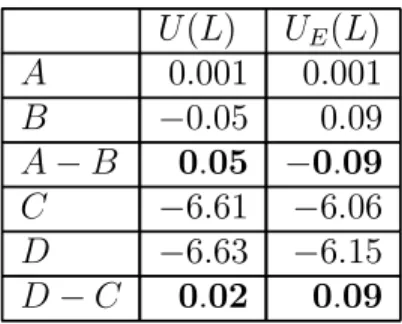
(15) UE (A) − UE (B) = 0.11u(1) − 0.10u(5) − 0.01u(0).. (12). Likewise, the difference between expected utilities of D and C is. UE (D) − UE (C) = 0.10u(5) + 0.01u(0) − 0.11u(1).. (13). In other words, these expected utility differences have the opposite sign. UE (A) − UE (B) = − (UE (D) − UE (C)) .. (14). Thus, according to expected utility, if a person prefers A to B, it is impossible that he prefers D to C. Here is a resolution of the paradox. Since the potential payoffs are so large compared to the resources of most players, suppose that the lotteries are only offered once: n = 1. To reflect decreasing marginal utility of money, let the utility of each outcome b = {0, 1, 5} be logarithmic: u(b) = ln(v+b), where v > 0 is. a constant that reflects player’s resources. I set v = 10−3 , which. 15.

(16) A B A−B C D D−C. U (L) UE (L) 0.001 0.001 −0.05 0.09 0.05 −0.09 −6.61 −6.06 −6.63 −6.15 0.02 0.09. Table 3: Allais utilities as estimated under asymmetric quadratic (type 2) loss, and by expected value. The paradox disappears under asymmetric loss.. corresponds to the player having about a thousand dollars. Under quadratic loss with c2 = 3.0, the paradox disappears. Refer to table 3 which shows that A is in fact preferred to B at the same time as D is preferred to C. According to the model developed here, I predict that if people are explicitly told that they can play the lotteries a very large number of times, then they will make choices consistent with expected utility. 3.2. Ellsberg paradox. Here is a usual statement of the Ellsberg paradox. An urn contains 300 balls: 100 are red; of the rest, some are blue and some are green. A person draws a random ball from the urn and is asked to choose between the following lotteries:. 16.

(17) Gamble A Receive $1 if the ball is red. Gamble B Receive $1 if the ball is blue. He also has to choose between the following two lotteries: Gamble C Receive $1 if the ball is not red. Gamble D Receive $1 if the ball is not blue. People usually prefer A to B and C to D. However, if we use expected utility theory, it appears that a person who prefers A to B has to also prefer D to C. Let pR be the probability of a red ball and pN R be the probability that the ball is not red. Then, under expected utility theory, preferring A to B implies that, in the person’s view, pR > pB . But preferring C to D implies that, in his view, pN R > pN B . Since pN R = 1 − pR , both of these inequalities cannot be true. The key to resolving this paradox is to realize that people are not estimating probabilities at all, they are estimating lotteries. Consider these lotteries with the model presented in this paper. A person plans to play his chosen lottery n times; xR is the number of times he draws a red ball. Letting the utility of no payment be zero, u (0) = 0, the random utility of A is 17.

(18) Ũ(A) =. xR u(1). n. (15). The estimate of this utility is the same thing but with xR replaced by its estimate x̂R . Thus, utilities of A and B are. x̂R u (1) n x̂B u (1) U (B) = n. (16). U (A) =. (17). Since drawing any ball is equally likely, the person knows that the probability of a red ball is pR =. 100 300. = 13 . From this,. he knows the distribution of the number of red draws xR : it is Binomial with parameters n and pR = 13 . µ ¶ 1 . xR ∼ B n, pR = 3. (18). On the other hand, he does not know the probability of a blue ball pB . The person might believe that the probability pB is distributed according to some probability function. Since probability pB can be anything between 0 and 23 , the person might think that pB is distributed Uniformly between 0 and 23 . If f (pB ) is the probability density of pB , then the distribution 18.

(19) of the number of blue balls is. f (xB ) =. Z. 2 3. B (n, pB ) f (pB ) dpB .. (19). 0. If f (pB ) is in fact Uniform, the expected number of red draws xR is equal to the expected number of blue draws xB : E [xR ] = E [xB ]. However, the variance of blue draws is greater than the variance of red draws: V ar (xB ) > V ar (xR ). This is because the probability of red draws is certain, while the probability of blue draws is not. The added uncertainty adds to the variance. Under asymmetric loss, with equal expected values and unequal variances, the estimate x̂B is less than x̂R . Because of this, the person prefers A over B. The same logic applies to the second pair of lotteries. Let xN R be the number of non-red draws. Then, because of equal expected values and unequal variances, the estimate of the number of non-blue draws is less than the estimate of the number of non-red draws: x̂N B < x̂N R . And so, U(A) > U(B) and U (C) > U (D). As a numerical example, let’s say that u(1) = 1, u(0) = 0, and the number of games is n = 20. I use quadratic loss with risk aversion c2 = 3.0. The lottery utilities are shown in table 19.

(20) A B A−B C D C −D. U(L) 0.29 0.24 0.05 0.62 0.57 0.05. Table 4: Ellsberg utilities.. 4. As the table shows, A is preferred to B while C is preferred to D. 3.3. St. Petersburg paradox. Here is a discussion of the St. Petersburg paradox based on (Martin 2001). A fair coin is flipped until it comes up heads for the first time. Let k be the toss on which this happens. Then, the St. Petersburg lottery pays $2k . The question is, how much would someone be willing to pay for playing this lottery? The expected value of the lottery is infinite: 1 1 EV = 21 + 22 + . . . = ∞. 2 4. (20). From this, it might appear that people would be willing to pay an infinite amount of money for the lottery, which is obviously wrong. One flaw with the above presentation of the paradox is 20.

(21) that it is made in terms of payoffs, not utilities. In fact, the first solution of the paradox, proposed by Bernoulli, is that people perceive payoffs in terms of utilities which are increasing, but at a decreasing rate. Under this solution, the utility of the lottery is 1 ¡ ¢ 1 ¡ ¢ UE (L) = u 21 + u 22 + . . . < ∞. 2 4. (21). However, we can easily circumvent this solution by making the payoffs not 2k , but higher. If u−1 (·) is the inverse of the ¡ ¢ elementary utility function, let’s make the payoff u−1 2k . In this case, the expected utility of the lottery is infinite, and so. it appears, once again, that people should be willing to pay an infinite amount for it. Now, consider this lottery in the framework presented here. For simplicity, let the utility of an outcome be equal to the outcome: u(b) = b. Under quadratic (type 2) loss, the value of utility diverges to infinity, regardless of what the risk aversion c2 is. Under linear (type 1) loss with either risk neutrality or risk aversion (c1 ≥ 1), the utility U(L) is always 2. While this is one possible answer, it is rather uninteresting. It could be argued that the answer is simply an artifact of the fact that the linear 21.

(22) loss produces discontinuous estimates when applied to discrete distributions. Consider now a type of loss that is between the two types discussed above, namely, the type 1.5 loss. Under this loss function, the utility of the lottery converges to a value greater than 2. For example, if the number of games is n = 1 and the risk aversion is c1.5 = 1.7, the utility of the lottery converges to U(L) ≈ 3.85. 3.4. Equity premium puzzle. This section provides some insight into the Equity Premium Puzzle. The difference between the return on equities and the return on almost riskless bonds is called the equity premium. Because equities are risky while bonds are not, expected equity premium is positive. In the United States and some other countries, when viewed through the lens of various asset pricing models, the premium seems excessive. According to asset pricing models, which use expected utility theory, risk aversion required to sustain such a large premium is unrealistically high (Obstfeld & Rogoff 1996, p. 310). There are two possible explanations for this paradox: either the asset pricing models do not accurately describe human behavior, or people are, in fact, 22.

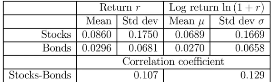
(23) extremely risk averse, at least in some situations. The classic paper on the subject is (Mehra & Prescott 1985). The paper examines real returns on stocks and almost riskless bonds between the years 1889 and 1978. The average real return on stocks was 6.98% per year, while on bonds, it was 0.8% per year. Thus, the equity premium is 6.98% − 0.8% = 6.18% per annum. But, according to asset pricing models, which use expected utility theory, under reasonable values of risk aversion, equity premium should not be greater than about 1% or 2%. Similarly large equity premiums are present in other data as well. (Shiller 2000) gives annual data on Stocks, Bonds, and the Consumer Price Index between the years 1871 and 1997.2 Stocks data consists of January values of the Standard and Poor’s Composite index and yearly dividend data for those stocks. Bonds data is the total nominal return from investing in January and then reinvesting in July at the six month prime commercial paper rate. Based on the (Shiller 2000) data, I calculate real returns for holding Stocks and Bonds. Rate r is the real annual return; Logarithm Return (LR) is ln (1 + r). The calculated statistics are in table 5. According to this data, the equity premium 2. Thanks to John Nuttall of University of Western Ontario for providing the data.. 23.

(24) Return r Log return ln (1 + r) Mean Std dev Mean µ Std dev σ Stocks 0.0860 0.1750 0.0689 0.1669 Bonds 0.0296 0.0681 0.0270 0.0658 Correlation coefficient Stocks-Bonds 0.107 0.129 Table 5: Returns on Stocks and Bonds from 1871 to 1997.. is 8.60% − 2.96% = 5.63%, still much greater than 2%. I use the model developed in this paper, with a relatively low value of risk aversion, to predict investor behavior in two cases: when the returns are as described by the data; and when returns are such that the equity premium is 2%. I find that the predicted investor behavior if returns are as observed seems reasonable, while behavior when equity premium is set to 2% seems very unreasonable. Suppose only two investment vehicles are available: Stocks and Bonds: V = {S, B}. In the minds of investors, the Logarithm Rates are Normally distributed with statistics as shown in table 5, and zero correlations across time. Each investor knows the number of years n that he will invest. For example, this could be the number of years to retirement. To simplify computations, I use the linear (type 1) loss function. Each investor knows his risk aversion c1 , which could be related to personal24.

(25) ity, family situation, and so on. I assume the relatively low risk aversion of c1 = 3.8 (see table 2 in section 2.2). For convenience, let t be the number of years until the investor stops investing (such as until retirement). Thus, the first year of investing is t = n while the last year is t = 1. Define the utility from investing is the logarithm of the total return. In other words,. Ũ = ln. n Y. (1 + rt ) =. t=1. n X. ln (1 + rt ) ,. (22). t=1. where rt is the real return that the investor receives in year t. Before the beginning of each year, investors decide what percentage of their money to put into each of the investment vehicles. They determine the optimal investment path by backward induction, as discussed in section 2.4. The utility is Normally distributed as follows:. Ũ ∼ N. Ã n X. µt ,. t=1. n X t=1. !. σ 2t ,. (23). where µt and σ t are mean and standard deviation of the Logarithm Return of the investment mix chosen for year t. If π V,t 25.

(26) is the fraction invested in V in year t, then. µt = σ 2t =. X. (24). π V,t µV. ÃV X. π 2V,t σ2V. V. !. + 2π S,t π B,t σ S σB ρSB. (25). The right hand side variables, µV , σ V , and ρSB , are taken from table 5. Figure 1 shows the proportion of money invested in Stocks, as a function of time remaining t, for a person with risk aversion c1 = 3.8; the rest of the money is held in Bonds. Until there are t = 21 years left, the person holds all his money in Stocks. Starting from t = 20, he gradually begins to shift from Stocks into Bonds. In t = 8, proportion invested in Stocks falls below 50%. During the last year of investing, when t = 1, the proportion is π S,1 = 22%. Now, suppose that, following asset pricing models, equity premium was 2%. That is, all the data is as is, except that the returns of Stocks rS are shifted by −E [rS ] + E [rB ] + 0.02. This changes the expected return on Stocks without changing their risk (standard deviation of return) or correlation to Bonds. 26.

(27) Figure 1: Optimal investment path under observed equity premium. Proportion invested in stocks versus years to retirement.. 27.

(28) The estimated mean of Logarithm Return for Stocks becomes µS = E [ln (1 + rS )] = 0.0339. Figure 2 shows the proportion of money invested in Stocks, as a function of t, under this scenario. Now, the person starts shifting into Bonds at t = 786; he starts investing less than 50% in Stocks at t = 312; he starts investing less than 20% in Stocks at t = 27. Such an investment path is very unrealistic.. 4. Hypothesis testing. In this section, I outline some ideas on how to apply the utility model presented in this paper to hypothesis testing. Hypothesis testing allows us to tell whether sufficient evidence exists for some proposition of interest. For example, based on data related to some quantity β, we might want to know if there is sufficient evidence that β > 0. The alternate hypothesis, HA , is the proposition for which we would like to know whether sufficient support exists; the null hypothesis, H0 , is the complement of the alternate. In this example, H0 : β ≤ 0; HA : β > 0. In conventional hypothesis testing, the size of the test is usually set to 5%; sometimes, it is also set to either 10% or 1%. The researcher sets the size of the test somewhat arbitrarily, without 28.

(29) Figure 2: Optimal investment path if equity premium was 2%. Proportion invested in stocks versus years to retirement.. 29.

(30) any direct reference to his attitude toward risk. Many times a null can be rejected at one common level, such as 5%, but not at another common level, such as 1%. In this situation in particular, the researcher has to have his preferences well-quantified. 4.1. The basic utility approach. Let B be a random variable, such as the response to some treatment. u (B) > 0 means that the response is desirable. B can take on M possible values, subscripted with m = 1, 2, . . . , M . A researches has already observed some values of this random variable. He wants to know that, if the treatment is applied in the future, the average utility of the treatment will be positive. The possible values of the random variable {bm } are known, but their probabilities pm are not. In observations, outcome bm occurs ym times. The researcher plans to apply this treatment n times. The utility of the treatment, Ũ (L), is the average perapplication utility. If the researcher’s estimate of this utility is positive, he concludes that, on average, the treatment produces desirable results; if the estimate is zero or negative, then the researcher concludes that, on average, the treatment produces undesirable results. The researcher explicitly accounts for his 30.

(31) attitudes toward risk in the estimation process by choosing an appropriate loss function. For simplicity, assume that the treatment, if chosen, will be applied a lot of times (n is very large). Then, the ratios. x n. reduce to the probabilities. But keep in mind that the probabilities themselves are not known but rather follow the Dirichlet distribution. The random variable utility becomes. Ũ (L) =. M X. pm u (bm ) .. (26). m=1. 4.2. Sample calculation. Suppose u (B) can be any integer between −10 and 10, all a priori equally likely. A researcher observes the utilities of k = 20 treatments. These observed utilities are: −10, −7, −6, −2, −2, −1, −1, 0, 2, 2, 5, 6, 6, 7, 8, 8, 9, 9, 9, 9. (27) The researches wants to know whether, if he applies the treatment a very large number of times, the average per-application utility will be positive. Let µ be the expected value of u (B). In the conventional hypothesis test framework, the researcher would test the following 31.

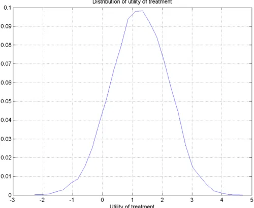
(32) hypothesis: H0 : µ ≤ 0; HA : µ > 0. Let µ̂ be the estimator of expected value µ, and let σ̂ be its (estimated) standard deviaµ̂ tion. A priori, if µ = 0, the ratio has the t distribution with σ̂ 20 − 1 = 19 degrees of freedom. From this, if the size of the test is 5%, the critical value of the test statistic is 1.73; if the size is 1%, the critical value is 2.54. The observed µ̂ is 2.55; the observed σ̂ = 1.30. The obtained test statistic is 1.97. Thus, the researcher accepts the hypothesis that µ > 0 at the 5% level, but not at the 1% level. It’s not clear what decision the researcher should make since there is no direct correspondence between the size of the test and the researcher’s attitudes toward risk. Now, let’s apply the approach developed above. Since a priori all outcomes are equally likely, set the prior parameter αm = 1 for all m. Figure 3 shows the distribution of utility of treatment, Ũ (L). The researcher calculates the point estimate of the utility, U (L), by specifying the parameters a and ca of the loss function that best reflect his preferences. In this example, the utility is positive under a wide range of very reasonable parameters. For instance, if the researcher has quadratic (type 2) loss with a moderate risk aversion of c2 = 13.1, then utility is U (L) = 0.3; 32.

(33) Figure 3: Distribution of utility for the sample calculation.. for a higher risk aversion of c2 = 22.4, utility is still positive at U (L) = 0.1. (See table 2 for risk aversion c2 .) A very high risk aversion of c2 = 52.5 does produce a negative utility of U (L) = −0.2 though. Whether the researcher decides that the treatment has a desirable effect depends directly on his easily quantifiable degree of risk aversion.. 33.

(34) 5. Conclusion. The utility model presented here is attractive theoretically since it is built upon solid probability principles. The model sheds light on several well-known paradoxes. The model can also be put to good use in hypothesis testing.. References Kahneman, D. & Tversky, A. (1979), ‘Prospect theory: An analysis of decision under risk.’, Econometrica 47, 263—291. Martin, R. (2001), The St. Petersburg paradox, in E. N. Zalta, ed., ‘The Stanford Encyclopedia of Philosophy (Fall 2001 Edition)’. URL: http://plato.stanford.edu/archives/fall2001/entries/paradoxstpetersburg/ Mehra, R. & Prescott, E. C. (1985), ‘The equity premium: A puzzle’, Journal of Monetary Economics 15, 145—162. Nuttall, J. (2003), ‘Comments on attempts to solve the equity premium puzzle’. URL: http://publish.uwo.ca/~jnuttall/equity.html 34.

(35) Obstfeld, M. & Rogoff, K. (1996), Foundations of International Macroeconomics, third edn, MIT Press. Shiller, R. J. (2000), Irrational Exuberance, Princeton University Press. URL: http://aida.econ.yale.edu/~shiller/books.htm Tversky, A. & Kahneman, D. (1981), ‘The framing of decisions and the psychology of choice.’, Science 211, 453 — 458.. 35.

(36)

No results found