Abstract— Computational fluid dynamics (CFD) was used to investigate heat transfer phenomena in a kerosene based ferrofluid. The flow is in a cylinder with height and diameter 3.5 mm and 75 mm, and the ferrofluid is treated as a two phase mixture of magnetic particles in a carrier phase. Different temperature gradients and uniform magnetic fields were applied over the geometry. Nusselt numbers were calculated as the heat transfer characteristic in the ferrofluid. Obtained results show that in the presence of aggregation of magnetic particles heat transfer will decrease, and Rayleigh rolls can not be observed.
Keywords—Ferrofluid, Nusselt number, Simulation.
I. INTRODUCTION
Ferrofluids are suspensions of small magnetic particles in appropriate carrier liquids such as kerosene [1]. Such fine particles may be coated by a suitable surfactant to keep a stable suspension state and they can be treated as particles of single magnetic domain. But some particles may combine to each other because of dipole-dipole interactions, and aggregations will produce [2].
Ferrofluids exert some unique performances under the influence of external magnetic fields, i.e. an applied magnetic field can be used to control physical and flowing properties of the ferrofluid [3]. Therefore they have a wide range of applications in a variety of fields like biomedicine and technology [1]. In most application cases, the flow and thermal phenomena inside the ferrofluid are involved [4].
Study of transport phenomena in ferrofluids involves use of computational fluid dynamics (CFD). Several recent publications have established the potential of CFD for describing the ferrofluids behavior like fluid motion and heat transfer [5]-[8].
Since the temperature gradient and the magnetic field strength are two vital factors affecting the flow and thermal behavior of ferrofluids, different cases contain combination of these factors have been simulated in this paper in order to
investigate their effects. In addition the influence of magnetic particle’s diameter on heat transfer is studied.
II. GOVERNING EQUATIONS
A. Mixture Model
Mixture model can predict the behavior of ferrofluids [1], [9], so this method is used in this study. The continuity, momentum, and energy equations for the mixture and the volume fraction equation for the secondary phases, as well as algebraic expressions for the relative velocities are as follow
( m) .
(
m m)
0t ρ ρ
∂
+ ∇ =
∂ v
(1)
(
)
(
)
2
( ) .
. ( )
m m m m m m m m
p p p Mp Mp c c Mc Mc m p
p P
t
m L V
ρ ρ μ
α ρ α ρ ρ α ξ
∂ + ∇ = −∇ + ∇ −
∂
∇ + + + ∇
v v v v
v v v v g H
(2)
(
)
(
)
, , ,
( m v mc T) . p p p p pc c c c p cc T . km T
t ρ α ρ α ρ
∂
+ ∇ + = ∇ ∇
∂ ⎡⎣ v v ⎤⎦
(3)
where , , ,ρ v P μ,ξ, ,H and k are density, velocity, pressure,
dynamic viscosity, Langevin parameter, magnetic field vector, and conductivity, respectively. Here subscripts m, p and c sequently refer to the mixture, magnetic particles and carrier fluid, and vMi =vi −vm is diffusion velocity. From the continuity equation for secondary phase, the volume fraction equation for magnetic phase can be obtained:
(
p p)
.(
p p(
m dr p,)
)
0t α ρ α ρ
∂
+ ∇ − =
∂ v v
(4)
wherev
dr p, is drift velocity. With considering to forces act ona single magnetic particle, the slip velocity is defined similar to [9]
(
)
2
( )
3 18
p p c
p
s p c
c p c
d m L
d
ρ ρ
ξ
πμ πμ
−
= − = ∇ +
v v v H g
(5)
Heat Transfer in the Kerosene-Based Ferrofluid
Using Computer Simulations
A. Jafari
1, T. Tynjälä
1, S.M. Mousavi
2,3, and P. sarkomaa
1where the stokes drag coefficient, valid for low Reynolds numbers, is applied. In this equation dpis the magnetic particle
diameter.
B. Magnetic Field Calculation
The conductivity of ferrofluids is usually very small, so Maxwell’s equations are as follow:
. 0,
∇ =B
(6) 0,
∇ ×H =
(7) where B is the magnetic induction which is related to the magnetization vector,M, and the magnetic field vector by the constitutive relation:
0( ),
μ
= +
B M H
(8) where μ0 is a magnetic permeability in vacuum. Magnetic scalar potential,φm, is defined as
m φ = −∇
H . (9)
Using Maxwell’s equations, the flux function for
magnetic scalar potential,
φm, can be written as
(
0)
(
0)
. 1 m . p p
p T T T
φ α α
α ∂ ∂ ∂ ∇ + ∇ = ∇ − + − ∂ ∂ ∂ ⎡⎛ ⎞⎤ ⎡⎛ ⎞⎤ ⎢⎜ ⎟⎥ ⎜ ⎟ ⎢⎝ ⎠⎥ ⎜ ⎟ ⎣ ⎦ ⎢⎣⎝ ⎠⎥⎦
M M M
H
(10)
where subscript 0 represents initial conditions and pand T
α are volume fraction of magnetic particles, and temperature, respectively. Within the simulations
0 , m T χ β ∂ = ∂ = − ∂ ∂
M M M
H and
p
M
α ∂
∂ are constant and using Langevin equation they can be defined as
(
)
0( )
0
2 0
1
1 coth ,
, p d
p T ξ α ξ α ξ ∂ = − + ∂
⎡
⎤
⎢
⎥
⎣
⎦
M MH H (11)
(
)
0( )
0
2
2 0
1
1 coth ,
, p p d
T T ξ α ξ α ξ ∂ = − − + ∂
⎡
⎤
⎢
⎥
⎣
⎦
M M H (12)( )
0 0 1 coth , dp T ξ
α ξ ∂ = − ∂
⎡
⎤
⎛
⎞
⎜
⎟
⎢
⎥
⎝
M⎠
H M⎣
⎦
(13)
where 0
( B )
m k T
μ
ξ = H , and ,m and kB are particle magnetic
moment and Boltzmann constant, respectively. Here
( )
p dL
α ξ
=
M M and saturation moment of bulk magnetic solid,Md, can be calculated from saturation magnetization of fluid byMs =αpMd.
III. NUMERICAL METHOD
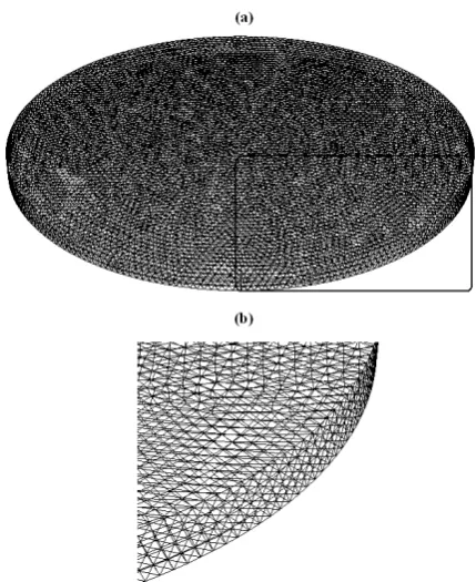
Commercial software, Gambit, was used to create the geometry and generate the grid. To divide the geometry into discrete control volumes, more than 105 tetrahedral computational cells, 2×10⁵ triangular elements, and
4
2.4 10× nodes were used. The grid is shown in Fig. 3.
Fig. 1: (a) The grid used in simulations, (b) To obtain better visualization the highlighted part in Fig. 1 (a) is magnified. A grid independency check has been conducted to ensure that the results are not grid dependent. To do this test, three different grids have been chosen. Their details and obtained numerical results at Ms =48 / ,kA m d =5.5 ,nm ΔTcritical =25 ,K and
25
T K
[image:2.595.323.538.186.449.2]Δ = are shown in table 1. The results appear to be grid independent. There was no significant variation in the nusselt number resulted by the grid with 2.1 10× 5mesh volume and those obtained from the fine grid, so the second grid was selected for all calculations.
Table 1: Effect of mesh on nusselt number after 200 s
Grid # 1 # 2 # 3
Number of nodes
3
1.9 10× 2.4 10× 4 5 10× 4 Mesh volume 1.2 10× 5 2.1 10× 5 2.5 10× 5
Nusselt
[image:2.595.300.554.644.726.2]The commercial code for computational fluid dynamics, Fluent, has been used for the simulations, and a user defined function was added to apply a uniform external magnetic field parallel to the temperature gradient . The finite volume method is adopted to solve three dimensional governing equations. The solver specifications for the discretization of the domain involve the presto, second-order upwind and first-order upwind for pressure, momentum and volume fraction, respectively. In addition for second-order upwind is used for energy. The under-relaxation factors, which are significant parameters affecting the convergence of the numerical scheme, were set to 0.3 for the pressure, 0.7 for the momentum, and 0.2 for the volume fraction. Using mentioned values for the under-relaxation factors a reasonable rate of convergence was achieved.
IV. RESULTS AND DISCUSSION
Simulations were done for a kerosene-based ferrofluid. Physical properties used in the simulations are the same as [9]. For the sake of simplicity, it is assumed that the effect of the magnetization variation due to the local temperature change of the ferrofluid is negligible because our main attention is to develop a numerical algorithm for the energy transport of a ferrofluid. Such assumption will not alter the intrinsic characteristic of the algorithm, but it simplifies the numerical computation.
[image:3.595.346.514.139.277.2]The magnetic fluid is in a cylinder with diameter and length 75 mm and 3.5 mm, respectively (as shown in Fig. 1). Constant temperature boundary conditions were applied for both bottom and top of the cylinder, and uniform external magnetic field was subjected parallel to the temperature gradient.
Fig. 2: The geometry used in this study
Temperature difference 28 K was applied between top and bottom of the cylinder. To estimate heat transfer performance of the ferrofluid, the local Nusselt number, Nu, is calculated at different values of magnetic fields in the presence and absence of natural convection. Obtained results show that heat transfer increases when temperature of bottom of the cylinder is higher. As Fig. 3 illustrates at the first of simulation effect of temperature gradient is more than magnetic field strength. This is also proved using Taguchi technique [10]. Note that in this paper when T
Tcritical
Δ
Δ is positive, it means that temperature of
bottom of the cylinder is higher and natural convection exists. Also negative sign represents absence of natural convection.
5.65 5.655 5.66 5.665 5.67 5.675 5.68
0 0.5 1
M/Ms
[image:3.595.307.552.488.722.2]Nu
Fig. 3: Nusselt number versus normalized magnetization after 1 s. Here Ms=18 / ,kA m d =5.5nm , and ΔTcritical =4.5K . Triangles and squares belong to T 6.2
Tcritical
Δ
Δ = and
6.2
T Tcritical
Δ
Δ = − , respectively.
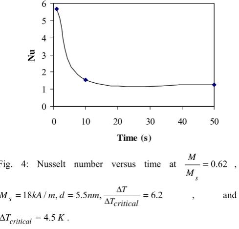
As Fig. 4 represents heat transfer of the ferrofluid depends on time. Strek and Jopek also referred to this in their paper [11]. With the geometry used in this study after 10 s the system becomes stable, and change of nusselt number with time is not significant. As Jafari et al. showed [9] with increase of aspect ratio, length to diameter of cylinder, instability in the system will increase.
0 1 2 3 4 5 6
0 10 20 30 40 50
Time (s)
Nu
Fig. 4: Nusselt number versus time at 0.62 s
M
M = ,
18 / , 5.5 , 6.2
s
T Tcritical
M kA m d nm Δ
Δ
= = = , and
4.5 critical
T K
Δ = .
[image:3.595.57.291.489.595.2]presented in Fig. 5. As can be expected with increase of temperature difference over the cylinder and strength of external magnetic field, heat transfer will improve. It is also found that after 0.5
s
M
M = heat transfer of the ferrofluid will
increase significantly.
1.2 1.22 1.24 1.26 1.28 1.3 1.32 1.34
0 0.5 1
M/Ms
Nu
Fig. 5: Nusselt number versus normalized magnetization after 50 s. Here Ms=48 / ,kA m d =5.5nm, and ΔTcritical =25K.
Triangles and squares belong to T 0.76
Tcritical
Δ
Δ = and
1.52
T Tcritical
Δ
Δ = , respectively.
Some times it is difficult to prevent aggregation in ferrofluids, so it has value to investigate its effect on the system. Similar simulations with higher diameter of magnetic particles were done and results are shown in Fig. 6. As this Fig. illustrates, formation of aggregates decrease the heat transfer characteristics of the ferrofluid.
1.26 1.27 1.28 1.29 1.3 1.31 1.32 1.33
0 0.2 0.4 0.6 0.8 1
M/Ms
[image:4.595.354.506.212.549.2]Nu
Fig. 6: Nusselt number versus normalized magnetization after
50 s. Here s 48 / , T 1.52
Tcritical
M kA m Δ
Δ
= = , and
25 critical
T K
Δ = . Triangles and squares belong to d =30nm
and d =5.5nm, respectively.
In order to better understanding the effect of aggregation on transfer phenomena flow pattern of the ferrofluid is studied. As Fig. 6 (a) illustrates in the presence of natural convection for smaller magnetic particles’ diameter Rayleigh rolls can be observed. This rotations increase heat transfer, and their effect on thermal convection in ferrofluids is important in certain chemical engineering and biochemical situations [12]. For
30
d= nm such kind of vortices did not recognize (Fig. 6 (b)).
Fig. 7: Velocity vectors after 50 s on a plane at z=0.00175 m, and for Ms=48 / ,kA m ΔTcritical =25K , and
0.76
T Tcritical
Δ
Δ = . (a) d =5.5nm, and (b) d =30nm.
V. CONCLUSION
[image:4.595.63.275.516.675.2]ACKNOWLEDGMENT
Authors gratefully acknowledge the Academy of Finland Grant No. 110852 for the support of this work.
REFERENCES
[1] T. Tynjälä, Theoretical and Numerical Study of Therrmomagnetic Convection in Magnetic Fluids. PhD Thesis, Finland: Lappeenranta University of Technology press, 2005.
[2] T. Tynjälä, A. Bozhko, P. Bulychev, G. Putin, and p. Sarkomaa, “On features of ferrofluid convection caused by barometrical sedimentation,” Journal of Magnetism and Magnetic Materials, vol. 300, 2006, pp. e195-e198.
[3] Y. Xuan, M. Ye, and Q. Li, “Mesoscale simulation of ferrofluid structure,” International Journal of Heat and Mass Transfer, vol. 48, 2005, pp. 2443–2451.
[4] Y. Xuan, Q. Li, and M. Ye, “Investigations of convective heat transfer in ferrofluid microflows using lattice-Boltzmann approach,” International Journal of Thermal Sciences, vol. 46, 2007, pp. 105-111.
[5] S. M. Snyder, T. Cader, and B. A. Finlayson, “Finite element model of magnetoconvection of a ferrofluid,” Journal of Magnetism and Magnetic Materials, vol. 262, 2003, pp. 269-279.
[6] C. Tangthieng, B. A. Finlayson, J. Maulbetsch, and T. Cader, “Heat transfer enhancement in ferrofluids subjected to steady magnetic fields,” Journal of Magnetism and Magnetic Materials, vol. 201, 1999, pp. 252-255.
[7] T. Tynjälä, A. Hajiloo, W. Polashenski, and P. Zamankhan,
“Magnetodissipation in ferrofluids,” Journal of Magnetism and Magnetic Materials, vol. 252, 2002, pp. 123–125.
[8] T. Tynjälä, and J. Ritvanen, “Simulations of thermomagnetic convection in an annulus between two concentric cylinders,” Indian Journal of Engineering and Material Sciences, vol. 11, 2004, pp. 283-288. [9] A. Jafari, T. Tynjälä, S. M. Mousavi,and P. Sarkomaa, “CFD simulation
of heat transfer in ferrofluids,” In Proceedings of European Congress of Chemical Engineering, Copenhagen, 16-20 September 2007.
[10] A. Jafari, T. Tynjälä, S. M. Mousavi, and P. Sarkomaa, “CFD simulation and evaluation of controllable parameters effect on Soret coefficient in ferrofluids using Taguchi technique, ” Journal of Computers andFluids,to be published.
[11] T. Strek, and H. Jopek, “Computer simulation of heat transfer through a ferrofluid,” Phys. Stat. Sol. (b), 2007, pp. 1–11 (DOI
0.1002/pssb.200572720).