Estimation of the long memory parameter in non stationary models: A Simulation Study

1

GREQAM

Groupement de Recherche en Economie Quantitative d'Aix-Marseille - UMR-CNRS 6579 Ecole des Hautes études en Sciences Sociales

Universités d'Aix-Marseille II et III

Document de Travail

n°2011-24

Estimation of the long memory parameter in

non stationary models: A Simulation Study

Mohamed Boutahar

Rabeh Khalfaoui

May 2011

Estimation of the long memory parameter in non stationary models:

A Simulation Study

M. Boutahar1, R. Khalfaoui2

Abstract

In this paper we perform a Monte Carlo study based on three well-known semiparametric estimates for the long memory fractional parameter. We study the efficiency of Geweke and Porter-Hudak, Gaussian semiparametric and wavelet Ordinary Least-Square estimates in both stationary and non stationary models. We consider an adequate data tapers to compute non stationary estimates. The

Monte Carlo simulation study is based on different sample size. We show that for d∈[1/4,1.25)

the Haar estimate performs the others with respect to the mean squared error. The estimation methods are applied to energy data set for an empirical illustration.

Key words: Wavelets, long memory, tapering, non-stationarity, volatility

1. Introduction

In recent years, studies about long memory have received the attention of statisticians and mathe-maticians. This phenomenon has grown rapidly and can be found in many fields such as hydrology, chimistry, physics, economic and finance. For instance, the studies of Diebold and Redebusch (1989) and Sowell (1992b) for real gross national product, Shea (1991) for interest rates, Lo (1991) and Willinger et al. (1995) for Ethernet traffic, Boutahar et al. (2007) for US inflation rate and Tsay (2009) for political time series. Moreover, Bollerslev and Mikkelsen (1996) proposed the FIGARCH model for modelling the persistence in the volatility in financial time series. The con-cept of long memory describes the property that many time series models possess, despite being stationary, higher persistence than short memory models, such as ARMA models.

Usually a long memory modelX_t can be characterized by a single memory parameterd∈(0,1/2)

called the degree of memory of the model, which controls the shape of the spectrum near zero frequency and the hyperbolic decay of its autocorrelation function. More precisely, the spectral

1_{M. Boutahar GREQAM, Université de la Méditerranée 2 rue de la charité, 13236, Marseille cedex 02, France}

e-mail: [email protected]

2_{R. Khalfaoui GREQAM, Université de la Méditerranée 2 rue de la charité, 13236, Marseille cedex 02, France}

e-mail: [email protected]

density, f_X(λ), of the long memory model is approximated in the neighborhood of the zero

fre-quency by

f_X(λ)∼cλ−2d asλ →0+, 0<c<∞. (1.1)

thus, f_X(λ)→∞asλ→0+. Under additional regularity assumptions of fX(λ),the autocorrelation

functionρ(k)of the long memory model has the following asymptotic behavior:

ρ(k)∼ck2d−1 ask→∞. (1.2)

As a consequence, for 0<d<1/2,∑−+∞∞|ρ(k)|=∞.This property of absolute nonsummability of

autocorrelations is often considered as definition of long memory and is satisfied by the ARFIMA models (Granger and Joyeux 1980 and Hosking 1981).

The properties of the model X_t depend on the parameter value d. Several estimation techniques

have been proposed in the literature for detecting the long memory phenomenon, in both time and frequency domains (Sowell 1992 and Beran 1994). These methods are grouped into three categories: the heuristic, the semiparametric and the parametric method. In the first group, we can cite for example Hurst (1951), Higuchi (1988) and Lo (1991). The second method focuses on the frequency domain estimation, in this context the most popular method is the one developed by Geweke and Porter-Hudak (1983). See also Reisen (1994), Chen et al. (1994), Robinson (1995a) and Robinson (1995b) among others. The third method based on the maximum likelihood function is proposed by Whittle (1951), Fox and Taqqu (1986), Dahlhaus (1989) and Sowell (1992). In

this class we estimate simultaneously all the parameters such as the long memory parameter d,

the short-runAR, theMAparameters and the scale parameter. Another semiparametric method for

estimating the long memory parameter is the so-called wavelet method proposed by McCoy and Walden (1996) and Jensen (1999a).

Some recent simulation studies comparing different techniques of estimation in stationary long memory models can be found in Taqqu et al. (1995), Reisen et al. (2006), Boutahar et al. (2007) and Tsay (2009).

We propose here a Monte Carlo study to compare the GPH, Gaussian semiparametric and wavelet OLS estimation method in both stationary and non stationary models. More specifically, our main objective is to determine the best estimation method of the long memory.

The rest of the paper is organized as follows. Section 2 describes the importance of fractional differencing. Section 3 briefly recalls definitions of long memory models. In section 4 we provide

a brief theoretical background of wavelets.3 Section 5 describes the GPH, the Local Whittle and

the wavelet estimation methods. Section 6 proposes a simulation study. An empirical application will be presented in section 7. Section 8 concludes.

3_{For a broader view of wavelet theory see Daubechies (1992, 1988), Mallat (1989) or Meyer (1993).}

2. Fractional differencing

2.1. Importance of fractional differencing

Most financial and economic time series are non-stationary, with their means and covariance fluctu-ating in time. Therefore, how to transform a non-stationary time series into a stationary one became an important problem in the field of time series analysis. The point of fractional differencing mod-els is not merely to allow for the memory measure to be fractional, but to allow it to be unknown, and estimated from data.

LetX_t be a time series, we can obtain a new seriesY_t by differencingX_t (i.e.Y_t = (1−L)dX_t). Let

f_Y(λ)be the spectral density ofYt. The spectral density ofXt is given by

f_X(λ) = 1−e iλ −2d f_Y(λ). (2.1)

2.2. Meaning of fractional differencing

The fractional differencing method proposed in this paper illustrates the essence of long-term

mem-ory. It shows the connection between differencing parameterdand long-term memory.

Consider the ARFIMA(0,d,0) model often called fractional white noise which can be expressed as

(1−L)dXt =εt where(1−L)d=∑∞_k=0δk(d)Lkand

δk(d) =

Γ(k−d)

Γ(k+1)Γ(−d), (2.2)

where Γ(.) denotes the gamma function. When d=0, Xt is merely a white noise, and its

auto-correlation function is equal to 0. When d =1, Xt is a random walk, whose value of

autocor-relation function is 1, and it can be regarded as a white noise after the first-order differencing.

Whendis non-integer,Xt=−∑+_k=∞₁δk(d)Xt−k+εt, and henceXtis influenced by all historical data

(Xt−1, Xt−2, . . .), this is just the characteristic of long-term memory.

3. Long memory

Researchers in several fields had noticed that the correlation between observations sometimes de-cayed at a slower rate than for data following classical ARMA models. Later on, as a direct result of the pioneer research of Mandelbrot and Van Ness (1968), self-similar and long memory models were introduced in the fields of statistics as a basis for inferences. Since then, this field is experienc-ing a considerable growth in the number of research results (for instance, see Franco and Reisen (2004); Boutahar et al. (2007); Reisen et al. (2006) and the references therein). The ARFIMA models are extension of ARMA models (short memory), thus we introduce a long memory charac-teristic by the fractional integration.

3.1. Definition and characteristics

A processXt,t≥0, is an ARFIMA(0,d,0) or I(d) model if:

(1−L)d(Xt−µ) =εt, (3.1)

whereεtis a white noise model anddis a real number such that|d|<1/2. This model is stationary

ford<1/2 and invertible ford>−1/2. Its Wold representation is given by:

X_t=µ+

+∞

∑

k=1

δk(−d)εt−k. (3.2)

where δk(d) is given by (2.2). For 0 <d <1/2, the autocorrelations decay hyperbolically like

k2d−1ask→+∞. Similarly, the spectral density of I(d) models behaves likeλ−2d asλ →0.

More generally, an ARFIMA(p,d,q) model is defined as:

Φ(L) (1−L)d(Xt−µ) =Θ(L)εt, (3.3)

whereεt∼i.i.d(0,σ_ε2)is a white noise process,Φ(L) =1−φ1L−. . .−φpLpandΘ(L) =1+θ1L+

. . .+θqLq.

The spectral density of the model{Xt}_t=1,...,T is

f(λ) = σ 2 ε 2π Θ(eiλ) Φ(eiλ) 2 1−e iλ −2d , for −π<λ <π. (3.4)

f(λ)is continuously differentiable for all non-zero frequencies. Ford>0, f(λ)is discontinuous

and unbounded at zero frequency. The principal properties of an ARFIMA(p,d,q) are as follows:

·ifd>−1/2,X_t is invertible,

·ifd<1/2,X_t is stationary,

·if−1/2<d<0, the autocorrelation functionρ(k)decreases more quickly than the case 0<d<1₂.

There is a stronger mean reversion, andX_tis called anti-persistent in Mandelbrot’s terminology.

·if 0<d< 1₂,X_t is a stationary long memory model. The autocorrelation function decays

hyper-bolically to zero and we have for|k| →∞,γ(k)≡Cγ(d,φ,θ)|k|

2d−1 where C_γ(d,φ,θ) = σ 2 ε π Θ(1) Φ(1) 2 Γ(1−2d)sin(πd), (3.5)

and then for|k| →∞,

ρ(k) = γ(k) γ(0)≡ C_γ(d,φ,θ) Rπ −π f(λ)dλ |k|2d−1. (3.6)

·ifd=1/2, the spectral density is unbounded at zero frequency.

3.2. Fractional gaussian noise

The fractional Gaussian noise (fGn) model was independently developed by Granger (1980), Granger and Joyeux (1980), and Hosking (1981). The best way to introduce the fGn model is to do it from

the fractional Brownian motion{B_H(t), t≥0}. 4

The fGn model{X_t, t≥0}is the increment of the fractional Brownian motion

X_t =B_H(t)−B_H(t−1), t≥1. (3.7)

Xt is a stationary Gaussian with autocovariance function

γ(k) =E(XtXt+k) = 1 2 h |k+1|2H−2k2H+|k−1|2Hi, k≥0. γ(k)∼H(2H−1)k2H−2, fork→∞andH6=1 2. (3.8)

withHis theself similarity parameter orHurst coefficient, 0<H<1.

The fGn model reduces to a white noise whenH =1/2, in this caseγ(k) =0 for allk≥1. When

1/2<H<1,X_t is a long memory model.

The spectral density of the fGn model is given by

f(λ) = CH 2 sinλ 2 2 +∞

∑

Wavelets are mathematical tools for analyzing time series. This method has been adopted in the areas of computational economics (see, for example, Davidson et al. 1998), then McCoy and

4_{Regular Brownian motion is a continuous time stochastic model,B(s), composed of independent Gaussian}

incre-ments. Mandelbrot and Van Ness (1968) also note that in a sense fractional Brownian motion,BH(s), can be regarded

as the approximation (0.5−H) fractional derivative of regular Brownian motion:

BH(s) = 1 Γ(H+1₂) Z s 0 (s−t)H−12_{dB(t) fors}∈_(0,1).

whereΓ(.)is the gamma function,B(t)is regular Brownian motion with unit variance andHis the Hurst coefficient,

originally due to Hurst (1951). The autocovariance of fractional Brownian motion is given by: E(BH(s)BH(t)) =

1 2

h

s2H+t2H− |s−t|2Hi.

Walden (1996) suggested an approximate maximum likelihood estimation method for estimating the fractional differencing parameter of a fractional white noise model. Johnstone and Silverman (1997) extended the method to an ARFIMA model. The series were decomposed (filtered) using wavelet transform. This analysis provides a time-frequency representation of a time series. It was developed to overcome the short coming of the Time Fourier Transform (TFT), which can be used to analyze non-stationary time series.

The Fourier transform can only provide frequency information that comprise the time series. It gives no direct information about when an oscillation occurred. However, wavelets can keep track of time and frequency information. The basic idea behind wavelet analysis is to decompose a time series into a number of components, each component can be associated with a particular scale at a particular time.

Generally, the wavelet refers to a set of functions of the form

ψsτ(t) =|s| −1/2 ψ t−τ s , (4.1)

where s is the dilation parameter (scaling parameter) which dilates or compresses a time series,

It is defined as |1/frequency| and corresponds to frequency information, and τ is the translation

parameter which simply moves the wavelet through the time domain.

Any function f ∈L2(_R)can be expanded into a wavelet series

f(t) = +∞

∑

∑

whereψjk∈L2(R)denotes thedilatedandtranslatedwavelet defined by

ψjk(t) =2j/2ψ 2jt−k

. (4.3)

for j,k∈_Z. The term jgives thescalecorresponding to adilationby 2j(theoctave), andk∈_Zis

the position or translation.

There are several wavelet families such as Haar, Daubechies, Shannon and so on. Daubechies (1992) constructed the hierarchy of the compactly supported and orthogonal wavelets with a desired degree of smoothness. This smoothness can be achieved by the number of vanishing moments

(the wavelet function ψ(t) has M vanishing moments if Rxrψ(t)dt =0, for r=0, . . . ,M−1).

Daubechies defined in her famous book Ten lectures on waveletsmany different types of wavelet

transform; the continuous wavelet transform, the discrete wavelet transform,... . In statistical setting researchs are more usually concerned with discret rather than continuous functions. In the following subsection we present a brief definition of discrete wavelet transform.

4.1. The Discrete Wavelet Transform

The wavelet transform is a function of scale in contrast to the Fourier transform which is a function of frequency. The scale is inversely proportional to a frequency interval. If the scale parameter

increases, then the wavelet basis is stretched in the time domain, shrunk in the frequency domain, and shifted toward lower frequencies. Conversely, a decrease in the scale parameter reduces the time support, increases the number of frequencies captured, and shifts toward higher frequencies. The wavelet method is essentially a transformation of time series data based on the two types of

filters called awavelet filterandscaling filter denoted byhandg, respectively. The wavelet filter

hand the scaling filtergare used to construct the Discrete Wavelet Transform (DW T) matrix. The

wavelet filterhof supportL∈_N(Lis the length of the filter), is defined so as to satisfy the following

three properties L

∑

∑

∑

∑

The scaling filter of supportLsimilarly satisfies the following three conditions :

L

∑

∑

∑

∑

The scaling filterg_i,i=1, . . . ,L, is the quadrature mirror filter corresponding to the wavelet filter

h_i,i=1, . . . ,Lby the relationship

g_i= (−1)i+1h_L−i−1. (4.4)

In addition, the following relation holds between the wavelet filterhand the scaling filterg

L

∑

i=1

g_ih_i+2n=0. (4.5)

LetX = (X₁, X₂, . . . ,X_T)0 be anT−vector of observations. Usually, the discrete wavelet transfor-mations are used with equally spaced observations with a simple size equal to an integer power of

2. Thus, we assume T =2J for some positive integer J. Using the wavelet filter and the scaling

filter, the original time seriesX_t,t =1, . . . ,T is transformed to the new seriesωj,t andνj,t, called

the wavelet and scaling coefficients, respectively. Then we can write

ω =W X. (4.6)

whereω is a T-vector wavelet coefficients andW isT×T real valued matrix called wavelet

trans-form matrix.5

4.2. Wavelet coefficients

TheDW T ofX= (X1, X2, . . . , XT) 0

can be performed using the so-called pyramid algorithm (Mal-lat 1989b).

•At first, the time seriesXt,t=1, . . . ,T withT =2J is filtered using the wavelet and scaling filters.

We obtain twoT/2-vectors of coefficients,ω1(wavelet coefficients) andν1(scaling coefficients).

The wavelet coefficients can be obtained by

ω1,t= L

∑

and the scaling coefficients can be obtained by

ν1,t = L

∑

•Second, the vector of scaling coefficients is filtered with both wavelet and scaling filter to obtain

a vector of wavelet and scaling coefficients ω2 andν2 each with length T/4. Thus, we filterν1,t

separately withhi,i=1, . . . ,Landgi,i=1, . . . ,Land subsample to produce two new series, namely

ω2,t = L

∑

∑

•Third, repeating this process recursively, afterJapplications ofDW T to get a wavelet and scaling

coefficients given by ωj,t = L

∑

∑

T. Orthonormality implies thatX=WTωandkωk2=kXk2, see Perceival and Walden (2000)

for more details.

After a brief overview of long memory phenomenon and wavelet analysis of time series, we present in the following section some estimation methods for the long memory parameter.

5. Estimation procedure

5.1. Stationary case

We deal with some well known estimation methods of the long memory parameter d. The first

one is the semiparametric method based on an approximated regression equation obtained from the logarithm of the spectral density function of a model. This method is proposed by Geweke and Porter-Hudak (1983). The second is the Gaussian semiparametric method developed by Robinson (1995b). The third is the wavelet method based on the discrete wavelet coefficients proposed by Abry and Veitch (1996) and Jensen (1999a).

5.1.1. GPH estimate

The GPH estimation procedure is a two-step procedure, which begins with the estimation of d.

This method is based on least squares regression in the spectral domain, exploits the sample form

of the pole of the spectral density at the origin: fX(λ)∼λ−2d,λ →0.To illustrate this method,

we can write the spectral density function of a stationary modelXt,t=1, . . . ,T as

f_X(λ) = 4 sin2(λ 2) −d f_ε(λ). (5.1)

where f_ε(λ)is the spectral density ofεt, assumed to be a finite and continuous function on the

in-terval[−π,π]; taking the logarithm of the spectral density function fX(λ),the log-spectral density

can be expressed as

log{fX(λ)}=log{fε(0)} −dlog

4 sin2(λ 2) +log f_ε(λ) f_ε(0) . (5.2)

LetI_X(λj)be the periodogram evaluated at the Fourier frequenciesλj=2πj/T, j=1,2, . . . ,m,T

is the number of observations and m is the number of considered Fourier frequencies, that is the

number of periodogram ordinates,6which will be used in the regression

logI_X(λj) = log{fε(0)} −dlog

4 sin2(λj 2 ) +log f_ε(λj) f_ε(0) +log I_X(λj) fX(λj) . (5.3)

6_{We can note that the chose of mis an important issue since it strongly affects estimation results. On the one}

hand,mshould be sufficiently small in order to consider only near zero frequencies. On the other hand,mshould be

sufficiently large to ensure convergence of OLS estimation.

where log{f_ε(0)}is a constant, log4 sin2(λj/2) is the exogenous variable and log

I_X(λj)/fX(λj)

is a disturbance error. The GPH estimate requires two major assumptions related to asymptotic

be-havior of the equation (5.3):

H1: for low frequencies, we suppose that logf_ε(λj)/fε(0) is negligible.

H2: the random variables logI_X(λj)/fX(λj) ,j=1, . . . ,mare asymptoticallyi.i.d.

Under the hypothesesH1andH2, we can write the linear regression

logI_X(λj) =α−dlog 4 sin2(λj 2 ) +e_j, (5.4)

whereej ∼i.i.d(−c,π2/6). 7 LetYj=−log

4 sin2(λj/2) , the GPH estimator is the OLS

esti-mate of the regression logIX(λj) on the constantα andYj. The estimate ofd, say ˆdGPH is

ˆ d_GPH =∑ m j=1 Yj−Y¯ logI_X(λj) ∑m_j=1 Yj−Y¯ 2 . (5.5)

where ¯Y =m−1∑m_j=1Yjandm=g(T)with lim_T→

∞

g(T) =∞and lim

T→∞

g(T)/T =0.

Geweke and Porter-Hudak (1983) showed that, ifT →∞and|d|<1/2 we have

√ m dˆ_GPH−d∼N  0, π2 6 ( m

∑

Porter-Hudak (1990), Crato and de Lima (1994), showed that the parameter m must be selected

so that m=Tυ_{, withυ =0.5, 0.6,0.7. Robinson (1995a), Hurvich et al. (1998), Tanaka (1999)}

and Lieberman et al. (2001) have analyzed the GPH estimate ˆdGPH in great detail. Under the

assumption of normality forXt, it has been proved that the estimate is consistent and asymptotically

normal, so that the estimated standard error of ˆdGPH can be used for inference. An alternative

semiparametric estimator has been proposed by Robinson (1995b).

5.1.2. Gaussian semiparametric estimate

The Gaussian semiparametric estimate called Local Whittle (LW) estimate was originally

devel-oped by Robinson (1995b) under the assumption thatXt,t=1, . . . ,T is a stationary model and its

spectral density behaves at low frequencies likeGλ−2d.8

Robinson (1995b) studied the Gaussian semiparametric estimate ofd based on minimization of a

local Whittle frequency domain log-likelihood,

`m(d,G) = 1 m m

∑

7_{cis Euler constant equal to 0.57721...}

8_{At low frequencies, the spectral density f}

X(λ)∼GX|λ|−2dasλ→0. for some finite constantGX>0.

wherem9 is some integer less thanT controlling the number of frequencies included in the local

likelihood. Given the interval of admissible estimate of d by, D= [∇1,∇2], where∇1 and∇2 are

numbers such that−1/2<∇1<∇2<1/2, theLW estimates are defined by

ˆ

d_mLW,GˆLW_m = arg min

d∈D,0<G<∞

`m(d,G). (5.8)

Concentrating equation (5.7) with respect toG, we obtain

ˆ d_mLW =arg min d∈D R_m(d). (5.9) where R_m(d) =logGLW_m (d) −2d1 m m

∑

∑

For linear time series with homoskedastic martingale difference innovations, with spectral density satisfying the same regularity conditions as for log-periodogram estimation based in GPH estimate,

Robinson (1995b) proved that ˆd_mLW is consistent and asymptotically normal

√ m dˆ_mLW−d→d N 0,1 4 . (5.11)

5.1.3. Wavelet OLS estimate

Let a time series X_t, t =1, . . . ,T follows a long memory model and let ψ(t) a wavelet function

satisfying

Z

ψ(t)dt =0, (5.12)

Z

trψ(t)dt =0, r=0, . . . ,M−1. (5.13)

Consider the family ofdilationsandtranslationsof the wavelet functionψ(t)defined by equation

(4.3). It can be shown that

Z

ψ2_jk(t)dt = Z

ψ2(t)dt. (5.14)

TheDW T of the modelXt,t=1, . . . ,T is then defined by

9_{The bandwithmsatisfies}

1 m+

m5log2m T4 →0.

if the approximation fX(λ)∼GX|λ|−2dhas errorO

|λ|2−2d

asλ→0.

ωjk=

Z

X_tψjkdt, for j, k∈Z. (5.15)

ifψ_jk are orthonormal basis,10 we obtain the following representation of the modelXt:

Xt = +∞

∑

∑

Consider theDW T coefficientsωjk discussed in subsection (4.2) and define the statistics

ˆ µj= 1 n_j nj

∑

wheren_j is the number of coefficients at octave javailable to be computed. As shown by Veitch

and Abry (1999). ˆ µj∼ z_j nj χ_n2_j. (5.18)

wherez_j=22d jc,c>0,andχ_n2_jis Chi-squared random variable withnjdegrees of freedom. Thus,

by taking logarithms we may write11

log₂µˆj∼2d j+log2c+

logχ_n2_j

log 2 −log2nj. (5.19)

Recall that the expected value and the variance of the random variable logχ_n2are given by

E logχ_n2 = ψ n 2 +log 2, (5.20) Var logχ_n2 = ζ 2,n 2 .

whereψ(z)is the psi function,ψ(z) =d/dzlog{Γ(z)}, andζ(2,n/2)is the Riemann zeta function

ζ(x) = 1 Γ(x) Z ∞ 0 ux−1 eu₋₁du= 1 1−21−s ∞

∑

The equation(5.19)can be written as

yj=α+βxj+εj, (5.22)

wherey_j=log₂µˆj−gj,α =logc,β =2d,xj=log2(2j) = jandεj=log2logχnj−log2nj−gj,

g_j=ψ nj/2

−log n_j/2. We conclude thatεj satisfies

10_{The family}

ψi j satisfies :Rψi j(t)ψkl(t) =0.

11_{see Veitch and Abry (1999) for details.}

E εj ≈ 0, (5.23) Var εj = ζ 2, nj 2 (log 2)2 ≈ 2njlog 2₂−1 .

In order to obtain a wavelet estimate, an OLS regression is fitted to points x_j,y_jfor j=1, . . . ,J

with weightsκj=nj.Thus, once the estimate ˆβ is obtained, an estimate for long memory parameter

dis given by ˆd=βˆ/2. Furthermore, an estimate of the variance of ˆdis provided by the estimate of

the variance of ˆβ,Var dˆ=1/4Var

ˆ

β

.

It is well known that under regularity conditions, the wavelet OLS estimate of d is efficient and

consistent.

5.2. Non-stationary case

It is necessary to extend the concept of long memory to the non-stationary framework, d ≥1/2.

Hurvich and Ray (1995) proposed a general model for possibly non-stationary integrated vector

models with componentsX_t,t=1, . . . ,T, each with memory parameterd>−1/2. So that, we say

X_t has memory parameterd>−1/2 ifY_t = (1−L)DX_t,D=bd+1/2c, is stationary with meanµ

and spectral density f_Y(λ)behaving as Gλ−2(d−D) around the origin, −1/2≤d−D≤1/2. To

estimate the memory parameter of an integrated model beyond the stationary regime (d>1/2), it

has been suggested to apply a data taper either to the time seriesX_t or to its D-th order difference

Y_t.

The idea of tapering in improving a Fourier approximation has a long history dating back to 1900 (see Brillinger, 1981). Tukey (1967) introduced this technique to time series for reducing the

periodogram bias due to the strong peaks and throughs in spectral density.12

Velasco (1999a, b)

A taper is a sequenceh_t,t=1, . . . ,T. Given a series ofT observations,X_t,t=1, . . . ,T, the tapered

discrete Fourier transform and the periodogram are defined as

DX(λj) = 2π T

∑

∑

The expectation of the periodogram is

12_{Tapering was originally used in nonparametric spectral analysis of short memory (d=0) time series in order}

to reduce bias due to frequency domain leakage, where part of the spectrum "leaks" into adjacent frequencies. The leakage is due to the discontinuity caused by the finitness of the sample and is reduced by using tapers which smooth this discontinuity.

EI_X(λj) =

Z π

−π

f_X(λ)K(λ−λj)dλ. (5.26)

where f_X(λ)is the spectral density ofXtdefined in (1.1) andK(λ) = (2πT)−1

∑T₁exp(iλt) 2 is the

Fejér kernel. Velasco (1999a) showed that whenX_t is non-stationary, f_X(λ)plays exactly the same

role as a spectral density in the asymptotics for the discrete Fourier transform at frequenciesλj,j6=

0 mod T and he showed that the periodogram is (asymptotically) unbiased forλ if j is growing

slowly withT andd<1.13 Velasco (1999a, b) and Velasco and Robinson (2000) have considered

several tapering schemes such as the cosine bell and Zurbenko-Kolmogorov tapers (Zurbenko,

1979). These tapers h_t,t =1, . . . ,T have the property of being orthogonal to polynomials up to

given order, for a subset of Fourier frequencies,

T

∑

1

1+t+. . .+tD−1h_teitλj_{=0, j∈ℑ}

D,T ⊂1, . . . ,T˜ , (5.27)

where ˜T = b(T−1)/2c. The usual discrete Fourier transform is obtained setting h_t ≡1,t =

1, . . . ,T, while the full cosine bell taper is given byh_t =1/2(1−cos[2πt/T]), and∑ht2=3T/8.

For sample sizeT =4N, whereN is an integer, the weightshP_t of the Parzen window14 are

h_tP=    21−2t−_TT 3 , 1≤t≤N or 3N≤t≤4N, 1−6h2t_T−T 2−2t−T T 3i , N<T <3N. (5.28)

Zurbenko (1979) used a class of data tapers h_tZ, t =1, . . . ,T suggested by Kolmogorov, indexed

by order p=1,2, . . . , assuming N=T/p integer. For p=3, Zurbenko’s weights are similar to

the cosine window, and when p=4,hZ_t are very close tohP_t. If p=2, Zurbenko taper is equal to

Bartlett’s triangular window15and when p=1 they are constant.

Hurvich and Chen (2000)

Hurvich and Chen (2000) have defined a family of data tapers. This family depends on a single

13_{See theorem 1 in Velasco (1999a) for more details.}

14_{The Parzen window is a piecewise curve window obtained by the convolution of two triangles of half length or}

four rectangles of one-four length.

w(n) =      1−6n−_NN_/2/22+6|n−_NN_/2/2|3,0≤ n−N₂ ≤N₄ 21−|n−_NN_/2/2|3, N₄ ≤n−N 2 ≤ n 2

n=0,1,2, . . . ,N−1, whereNis the length of the window.

15_{The Bartlett window of widthNalso known as triangular window is defined as}

w(n) =    1−2n N, 0≤n≤ N 2 1+2n_N, −N 2 ≤n≤0 0,otherwise

parameter p, referred to as the taper order. Seth_t =1−exp(2iπt/T) and for any integer p≥0,

define the tapered discrete Fourier transform of order pof the sequenceX_t, t∈_Zas follows:

D_Xp(λ) = (2πTap)−1/2 T

∑

wherea_p=n−1∑_tT=1|ht|2pis a normalization factor. As shown in Hurvich and Chen (2000, Lemma

0), the decay of the discrete Fourier transform of the taper of order pis given by

(2πTap)−1/2 T

∑

This property means that higher-order tapers control the leakage more effectively. The Fourier transform of the taper may be expressed as a finite sum of shifted Dirichlet kernels,

T

∑

∑

∑

Chen (2001) defined a new class of tapers. He proposed a linear combinations of Hurvich and Chen (2000) tapers with different phase shifts,

h(x) = 1−ei2πxp a₀+a₁ei2πx_{+. . .+a} q−1ei2(q−1)πx . (5.33) 5.2.1. GPH estimate

Under some smoothness conditions on the short-memory density function f∗, and by assuming that

the taper order pis larger thanD, the ratios of thepooled periodogram ofY_t divided by its spectral

density ¯I_τY_,p(λ˜j)/fY(λ˜j)arei.i.d.16 τ is the pooling order of the periodogram.

where ¯ I_τY_,p(λ˜j) = (p+τ)(l−1)+p

∑

∑

16_{See Faÿ et al. (2009)}

The parameter I_τX(λj) is the periodogram of X evaluated at the frequencies λj = 2πj/T, j =

1, . . . ,m. The log-periodogram estimate of Geweke and Porter-Hudak (1983) is defined as the least squares estimate in the linear regression model

loghI¯Y_τ,p(λ˜j) i =logf∗(0) + (d−D)Y_j+u_j,1≤ j≤m, (5.36) whereYj=−2 log 1−e iλ˜j anduj ∼ =log h ¯ I_τY_,p(λ˜j)/fX(λ˜j) i . The GPH estimate is ˆ d_GPH(m) = ∑ m j=1 Yj−Y¯ ∑mj=1 Yj−Y¯ 2×log h ¯ I_τY_,p(λ˜j) i +D (5.37)

Velasco (1999b) showed that the GPH estimate is consistent for d ∈[1/2,1) and asymptotically

normally distributed ford∈[1/2,3/4), the GPH estimate has non-normal limiting distribution for

d∈[3/4,1], and ford>1, it is consistent if p≥ bd+1/2c+1.

5.2.2. Local Whittle estimate

Let`p(G,d)be the objective function17

`_p(G,d) = p m _j=p,

∑

I(λj)is defined in (5.25). Define the lower and upper bound of the admissible estimates ofdby∇1

and∇2. ∇1and∇2are numbers such that−1/2<∇1<∇2<d∗, whered∗is the maximum value

ofdwe can estimate with tapers of order p. The estimates of(Gp,dp)are defined as

ˆ

Gp,dˆ_LWp = arg min

0<G<∞,d∈[∇1,∇2]

`(G,d) (5.39)

It can be shown that

ˆ d_LWp = arg min d∈[∇1,∇2] R_p(d), (5.40) where Rp(d) =logGp(d)−2d p m _j=p,

∑

∑

Velasco (1999a) showed that the LW estimate withτ=0 andD=0 is consistent ford∈(−1/2,1)

and asymptoticallyN(0,1/4)ford∈(−1/2,3/4). He showed that ifd>1 and p≥ bd+1/2c+1

the estimate is consistent. In the next section, we report the results of a Monte Carlo experiment based on the three estimation methods defined above.

6. Simulation study

In this section, a simulation study is used to assess the performance of the three estimation proce-dures. For this purpose we consider four models: ARFIMA(0,d,0), ARFIMA(1,d,0), ARFIMA(0,d,1)

and ARFIMA(1,d,1), d=0.05, 0.15, 0.25, 0.35, 0.45, 0.50, 0.75, 1.00, 1.25, 1.50. 1000

replica-tions of sample sizeT =28, 29, 210 are generated. The GPH method was applied using truncation

value m=T0.5. The realizations of ARFIMA(1,d,1) model were generated for same sample size

and of AR coefficient φ =0.2 and MA coefficient θ =0.1. Wavelet analysis is performed with

the Haar or D(2)18 and Daubechies filters with 2 and 4 vanishing moments. In the non stationary

case, for all estimators we have used the taper of order p=2 and p=3 of Bartlett and Zhurbenko

Kolmogorov, respectively.

Our aim is divided in three points: first, to show the efficiency of the estimates, we computed the

Bias and the Root Mean Squared Error of the estimates of long memory parameter d. Second,

to show the effect of choosing the wavelet filter in estimating the long memory parameter for stationary and non stationary times series. Third, to show the importance of data tapers in non stationary case.

To compare the different estimators we considered the Bias given by Bias=d¯−d, where ¯d =

1 n∑

n

i=1dˆi and the Root Mean-Squared Error value, denoted hereafter by RMSE , i.e, RMSE =

q 1 n∑ n i=1 dˆi−d 2 .

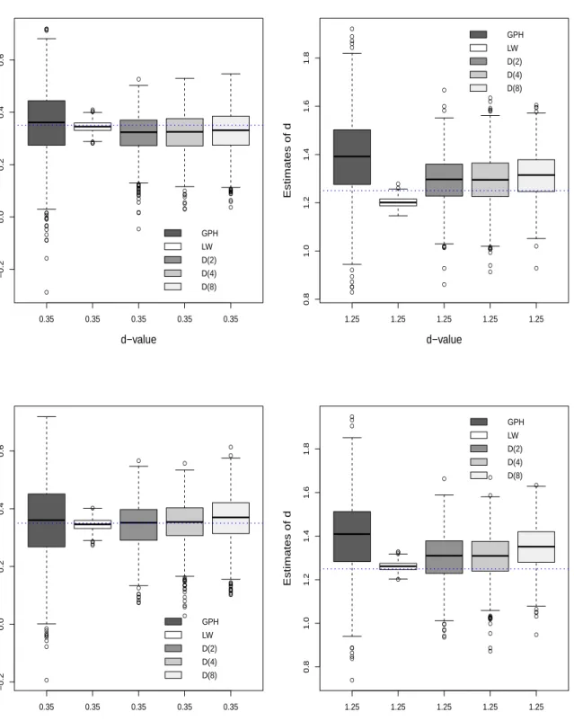
The boxplots for the ARFIMA(0,d,0) and ARFIMA(1,d,1) models withd=0.35 (stationary case)

andd=1.25 (non stationary case) are given in figures 6.3.

TheRMSEandBiasfor the GPH, LW and wavelet OLS estimates over 1000 simulated realizations

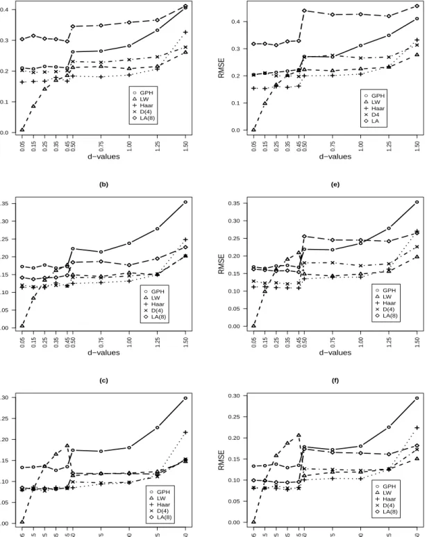
are provided in table 6.1, 6.2, 6.3 and 6.4. Some general comments are as follows :

•In stationary case, for the four models the LW estimate performs the GPH estimate (smallRMSE).

Such results were pointed out in Boutahar et al. (2007). In non stationary case, we have found the same results.

•Generally, for the four models used in our simulation and ford≤0.2, the LW estimate is better

than the wavelet OLS one.

• Increasing the number of vanishing moments, we showed that the LW estimate is better. For

instance, for the LA(8) estimate (the number of vanishing moments is 4) the RMSEis larger than

those of all estimates.

18_{The Haar filter corresponds to the Daubechies filter with one vanishing moments.}

Figure 6.1. RMSEas a function ofdfor ARFIMA(0,d,0) and ARFIMA(1,d,0) models. ● ● ● ● ● ● ● ● ● ● (a) ● GPH LW Haar D(4) LA(8) 0.05 0.15 0.25 0.35 0.45 0.50 0.75 1.00 1.25 1.50 0.0 0.1 0.2 0.3 0.4 d−values RMSE ● ● ● ● ● ● ● ● ● ● (d) ● GPH LW Haar D4 LA 0.05 0.15 0.25 0.35 0.45 0.50 0.75 1.00 1.25 1.50 0.0 0.1 0.2 0.3 0.4 d−values RMSE ● ● ● ● ● ● ● ● ● ● (b) ● GPH LW Haar D(4) LA(8) 0.05 0.15 0.25 0.35 0.45 0.50 0.75 1.00 1.25 1.50 0.00 0.05 0.10 0.15 0.20 0.25 0.30 0.35 d−values RMSE ● ● ● ● ● ● ● ● ● ● (e) ● GPH LW Haar D(4) LA(8) 0.05 0.15 0.25 0.35 0.45 0.50 0.75 1.00 1.25 1.50 0.00 0.05 0.10 0.15 0.20 0.25 0.30 0.35 d−values RMSE ● ● ● ● ● ● ● ● ● ● (c) ● GPH LW Haar D(4) LA(8) 0.05 0.15 0.25 0.35 0.45 0.50 0.75 1.00 1.25 1.50 0.00 0.05 0.10 0.15 0.20 0.25 0.30 d−values RMSE ● ● ● ● ● ● ● ● ● ● (f) ● GPH LW Haar D(4) LA(8) 0.05 0.15 0.25 0.35 0.45 0.50 0.75 1.00 1.25 1.50 0.00 0.05 0.10 0.15 0.20 0.25 0.30 d−values RMSE

Notes: RMSEas a function of long memory parameter using GPH, LW and wavelet OLS (Haar,

D(4) and LA(8)) estimation methods. (a), (b), (c) for an ARFIMA(0,d,0); (d), (e) and (f) for an

ARFIMA(1,d,0) models, withT =256,T =512 andT =1024.

Figure 6.2. RMSEas a function ofdfor ARFIMA(0,d,1) and ARFIMA(1,d,1) models. ● ● ● ● ● ● _● ● ● ● (g) ● GPH LW Haar D(4) LA(8) 0.05 0.15 0.25 0.35 0.45 0.50 0.75 1.00 1.25 1.50 0.1 0.2 0.3 0.4 d−values RMSE ● ● ● ● ● ● ● ● ● ● (j) ● GPH LW Haar D(4) LA(8) 0.05 0.15 0.25 0.35 0.45 0.50 0.75 1.00 1.25 1.50 0.0 0.1 0.2 0.3 0.4 d−values RMSE ● _{● ● ●} ● ● _● ● ● ● (h) ● GPH LW Haar D(4) LA(8) 0.05 0.15 0.25 0.35 0.45 0.50 0.75 1.00 1.25 1.50 0.00 0.05 0.10 0.15 0.20 0.25 0.30 0.35 d−values RMSE ● ● ● ● ● ● ● ● ● ● (k) ● GPH LW Haar D(4) LA(8) 0.05 0.15 0.25 0.35 0.45 0.50 0.75 1.00 1.25 1.50 0.00 0.05 0.10 0.15 0.20 0.25 0.30 0.35 d−values RMSE ● _{● ● ●} ● ● _● ● ● ● (i) ● GPH LW Haar D(4) LA(8) 0.05 0.15 0.25 0.35 0.45 0.50 0.75 1.00 1.25 1.50 0.00 0.05 0.10 0.15 0.20 0.25 0.30 0.35 d−values RMSE ● ● ● ● ● ● ● ● ● ● (l) ● GPH LW Haar D(4) LA(8) 0.05 0.15 0.25 0.35 0.45 0.50 0.75 1.00 1.25 1.50 0.00 0.05 0.10 0.15 0.20 0.25 0.30 d−values RMSE

Notes: RMSEas a function of long memory parameter using GPH, LW and wavelet OLS (Haar,

D(4) and LA(8)) estimation methods. (g), (h), (i) for an ARFIMA(0,d,1); (j), (k) and (l) for an

ARFIMA(1,d,1) models, withT =256,T =512 andT =1024.

Figure 6.3. Box-plots of GPH, LW and wavelet OLS estimators. ● ● ● ● ● ● ● ● ● ● ● ● ● ● ● ● ● ● ● ● ● ● ● ● ● ● ● ● ● ● ● ● ● ● ● ● ● ● ● ● ● ● ● ● ● ● ● ● ● ● ● ● ● ● ● ● ● ● ● ● ● ● ● 0.35 0.35 0.35 0.35 0.35 −0.2 0.0 0.2 0.4 0.6 d−value Estimates of d GPH LW D(2) D(4) D(8) ● ● ● ● ● ● ● ● ● ● ● ● ● ● ● ● ● ● ● ● ● ● ● ● ● ● ● ● ● ● ● ● ● ● ● ● ● ● ● ● ● ● 1.25 1.25 1.25 1.25 1.25 0.8 1.0 1.2 1.4 1.6 1.8 d−value Estimates of d GPH LW D(2) D(4) D(8) ● ● ● ● ● ● ● ● ● ● ● ● ● ● ● ● ● ● ● ● ● ● ● ● ● ● ● ● ● ● ● ● ● ● ● ● ● ● ● ● ● ● ● ● ● ● ● ● ● ● ● ● ● ● ● ● 0.35 0.35 0.35 0.35 0.35 −0.2 0.0 0.2 0.4 0.6 d−value Estimates of d GPH LW D(2) D(4) D(8) ● ● ● ● ● ● ● ● ● ● ● ● ● ● ● ● ● ● ● ● ● ● ● ● ● ● ● ● ● ● ● ● ● ● ● ● ● ● ● ● 1.25 1.25 1.25 1.25 1.25 0.8 1.0 1.2 1.4 1.6 1.8 d−value Estimates of d GPH LW D(2) D(4) D(8)

Notes: The results are based on 1000 realizations with sample sizeT=1024 for an ARFIMA(0,d,0)

and ARFIMA(1,d,1) model. The dotted blue lines indicate 0.35 and 1.25 ordinates, respectively. The

first row of the picture corresponds to the ARFIMA(0,d,0) model and the second row corresponds to the ARFIMA(1,d,1) model.

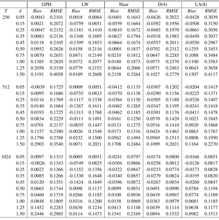
Table 6.1. Bias and RMSE of the GPH, LW and wavelet OLS estimator of the long memory parameter for an ARFIMA(0,d,0).

GPH LW Haar D(4) LA(8)

T d Bias RMSE Bias RMSE Bias RMSE Bias RMSE Bias RMSE

256 0.05 -0.0043 0.2101 0.0018 0.0084 -0.0401 0.1643 -0.0426 0.2022 -0.0428 0.3039 0.15 0.0021 0.2072 -0.0759 0.0851 -0.0559 0.1664 -0.0392 0.1956 -0.0508 0.3150 0.25 -0.0047 0.2152 -0.1181 0.1410 -0.0610 0.1672 -0.0485 0.1970 -0.0661 0.3056 0.35 0.0083 0.2136 -0.1348 0.1695 -0.0627 0.1794 -0.0518 0.1983 -0.0450 0.3037 0.45 0.0118 0.2105 -0.1399 0.1853 -0.0664 0.1674 -0.0557 0.2011 -0.0550 0.2967 0.50 0.0952 0.2626 0.0158 0.2116 -0.0001 0.1837 0.0702 0.2312 0.1255 0.3453 0.75 0.0870 0.2651 0.0471 0.2149 0.0210 0.1812 0.0647 0.2285 0.1088 0.3484 1.00 0.1385 0.2820 0.0372 0.2077 0.0180 0.1873 0.0575 0.2370 0.1100 0.3583 1.25 0.2058 0.3330 0.0779 0.2152 0.0644 0.2066 0.0571 0.2463 0.0643 0.3658 1.50 0.3191 0.4058 0.0109 0.2608 0.2158 0.3264 0.1027 0.2779 0.1507 0.4117 512 0.05 -0.0039 0.1725 0.0009 0.0051 -0.0412 0.1135 -0.0307 0.1202 -0.0204 0.1415 0.15 0.0095 0.1686 -0.0755 0.0833 -0.0370 0.1138 -0.0290 0.1156 -0.0225 0.1371 0.25 0.0116 0.1769 -0.1117 0.1338 -0.0384 0.1130 -0.0305 0.1188 -0.0326 0.1407 0.35 0.0140 0.1684 -0.1267 0.1611 -0.0482 0.1265 -0.0347 0.1195 -0.0241 0.1418 0.45 0.0193 0.1725 -0.1313 0.1768 -0.0462 0.1185 -0.0301 0.1176 -0.0411 0.1478 0.50 0.0834 0.2229 -0.0111 0.1491 0.0161 0.1250 0.0570 0.1420 0.1023 0.1845 0.75 0.0701 0.2137 -0.0035 0.1447 0.0133 0.1275 0.0516 0.1410 0.0920 0.1868 1.00 0.1157 0.2380 0.0026 0.1548 0.0173 0.1316 0.0424 0.1463 0.0863 0.1767 1.25 0.1796 0.2788 0.0232 0.1500 0.0562 0.1494 0.0569 0.1513 0.0808 0.1950 1.50 0.2903 0.3540 0.0071 0.2021 0.1708 0.2484 0.1099 0.2021 0.1164 0.2270 1024 0.05 0.0097 0.1333 0.0005 0.0031 -0.0241 0.0797 -0.0174 0.0800 -0.0166 0.0851 0.15 -0.0026 0.1343 -0.0749 0.0825 -0.0304 0.0866 -0.0258 0.0812 -0.0126 0.0817 0.25 0.0022 0.1366 -0.1152 0.1356 -0.0322 0.0847 -0.0233 0.0774 -0.0173 0.0828 0.35 0.0085 0.1266 -0.1330 0.1648 -0.0340 0.0857 -0.0279 0.0824 -0.0195 0.0820 0.45 0.0120 0.1351 -0.1424 0.1849 -0.0396 0.0872 -0.0267 0.0834 -0.0260 0.0847 0.50 0.0663 0.1744 0.0098 0.1137 0.0099 0.0851 0.0491 0.0990 0.0784 0.1194 0.75 0.0460 0.1719 0.0266 0.1185 0.0100 0.0936 0.0419 0.0967 0.0774 0.1189 1.00 0.0848 0.1805 0.0316 0.1200 0.0158 0.0969 0.0383 0.0979 0.0681 0.1185 1.25 0.1452 0.2283 0.0438 0.1234 0.0413 0.1148 0.0439 0.1114 0.0638 0.1177 1.50 0.2446 0.2985 0.0114 0.1473 0.1541 0.2169 0.0894 0.1532 0.0982 0.1513

•For 0.5≤d<1.5, we have used the Bartlett taper of order p=2. We found that the Haar filter

performs better results than the GPH, LW, D(4) and LA(8) estimates. But, for d ≥1.5 we have

used the Zhurbenko Kolmogorov taper of order p=3. Using the Zhurbenko Kolmogorov taper the

D(4) is better than the GPH, Haar and LA(8) estimates. Hence, we have smallRMSE.

•In non stationary case, ford≥1.5 the LW estimate is better than all other estimates.

We concluded that theRMSEof the LW estimate are smaller than those of GPH and wavelet OLS

Table 6.2. Bias and RMSE of the GPH, LW and wavelet OLS estimator of the long memory parameter for an ARFIMA(1,d,0).

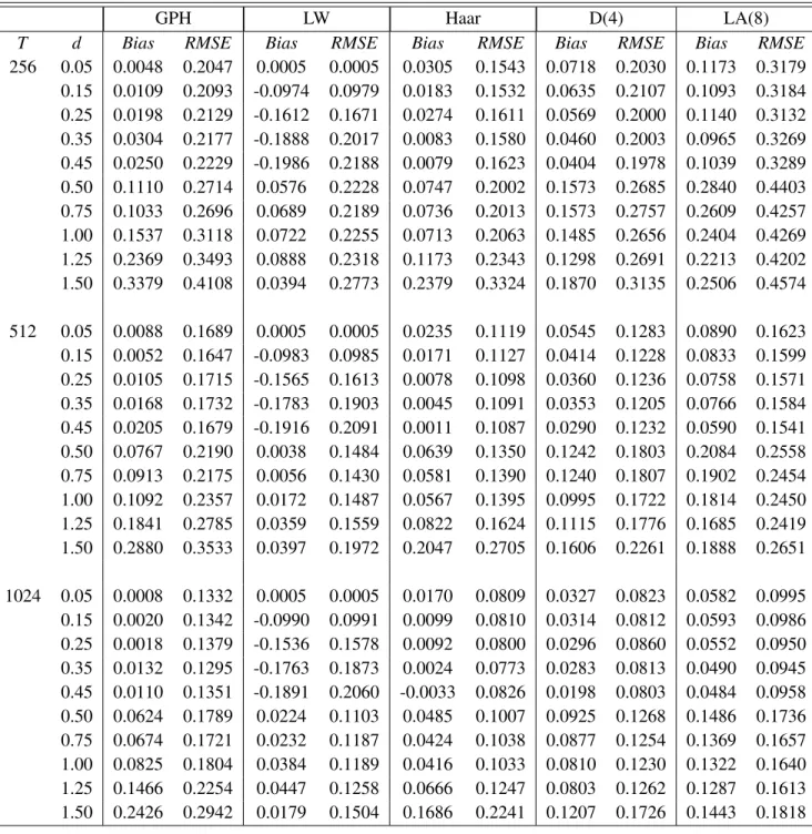
GPH LW Haar D(4) LA(8)

T d Bias RMSE Bias RMSE Bias RMSE Bias RMSE Bias RMSE

256 0.05 0.0048 0.2047 0.0005 0.0005 0.0305 0.1543 0.0718 0.2030 0.1173 0.3179 0.15 0.0109 0.2093 -0.0974 0.0979 0.0183 0.1532 0.0635 0.2107 0.1093 0.3184 0.25 0.0198 0.2129 -0.1612 0.1671 0.0274 0.1611 0.0569 0.2000 0.1140 0.3132 0.35 0.0304 0.2177 -0.1888 0.2017 0.0083 0.1580 0.0460 0.2003 0.0965 0.3269 0.45 0.0250 0.2229 -0.1986 0.2188 0.0079 0.1623 0.0404 0.1978 0.1039 0.3289 0.50 0.1110 0.2714 0.0576 0.2228 0.0747 0.2002 0.1573 0.2685 0.2840 0.4403 0.75 0.1033 0.2696 0.0689 0.2189 0.0736 0.2013 0.1573 0.2757 0.2609 0.4257 1.00 0.1537 0.3118 0.0722 0.2255 0.0713 0.2063 0.1485 0.2656 0.2404 0.4269 1.25 0.2369 0.3493 0.0888 0.2318 0.1173 0.2343 0.1298 0.2691 0.2213 0.4202 1.50 0.3379 0.4108 0.0394 0.2773 0.2379 0.3324 0.1870 0.3135 0.2506 0.4574 512 0.05 0.0088 0.1689 0.0005 0.0005 0.0235 0.1119 0.0545 0.1283 0.0890 0.1623 0.15 0.0052 0.1647 -0.0983 0.0985 0.0171 0.1127 0.0414 0.1228 0.0833 0.1599 0.25 0.0105 0.1715 -0.1565 0.1613 0.0078 0.1098 0.0360 0.1236 0.0758 0.1571 0.35 0.0168 0.1732 -0.1783 0.1903 0.0045 0.1091 0.0353 0.1205 0.0766 0.1584 0.45 0.0205 0.1679 -0.1916 0.2091 0.0011 0.1087 0.0290 0.1232 0.0590 0.1541 0.50 0.0767 0.2190 0.0038 0.1484 0.0639 0.1350 0.1242 0.1803 0.2084 0.2558 0.75 0.0913 0.2175 0.0056 0.1430 0.0581 0.1390 0.1240 0.1807 0.1902 0.2454 1.00 0.1092 0.2357 0.0172 0.1487 0.0567 0.1395 0.0995 0.1722 0.1814 0.2450 1.25 0.1841 0.2785 0.0359 0.1559 0.0822 0.1624 0.1115 0.1776 0.1685 0.2419 1.50 0.2880 0.3533 0.0397 0.1972 0.2047 0.2705 0.1606 0.2261 0.1888 0.2651 1024 0.05 0.0008 0.1332 0.0005 0.0005 0.0170 0.0809 0.0327 0.0823 0.0582 0.0995 0.15 0.0020 0.1342 -0.0990 0.0991 0.0099 0.0810 0.0314 0.0812 0.0593 0.0986 0.25 0.0018 0.1379 -0.1536 0.1578 0.0092 0.0800 0.0296 0.0860 0.0552 0.0950 0.35 0.0132 0.1295 -0.1763 0.1873 0.0024 0.0773 0.0283 0.0813 0.0490 0.0945 0.45 0.0110 0.1351 -0.1891 0.2060 -0.0033 0.0826 0.0198 0.0803 0.0484 0.0958 0.50 0.0624 0.1789 0.0224 0.1103 0.0485 0.1007 0.0925 0.1268 0.1486 0.1736 0.75 0.0674 0.1721 0.0232 0.1187 0.0424 0.1038 0.0877 0.1254 0.1369 0.1657 1.00 0.0825 0.1804 0.0384 0.1189 0.0416 0.1033 0.0810 0.1230 0.1322 0.1640 1.25 0.1466 0.2254 0.0447 0.1258 0.0666 0.1247 0.0803 0.1262 0.1287 0.1613 1.50 0.2426 0.2942 0.0179 0.1504 0.1686 0.2241 0.1207 0.1726 0.1443 0.1818

estimates for d ≤ 0.2 and d ≥1.5. Thus, the LW estimation method has a good performance.

Moreover, the performance of the Haar estimate is better for 0.3≤d<1.5.

Table 6.3. Bias and RMSE of the GPH, LW and wavelet OLS estimator of the long memory parameter for an ARFIMA(0,d,1).

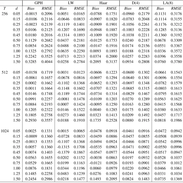
GPH LW Haar D(4) LA(8)

T d Bias RMSE Bias RMSE Bias RMSE Bias RMSE Bias RMSE

256 0.05 -0.0015 0.2096 0.0051 0.0165 -0.0788 0.1751 -0.0960 0.2179 -0.1131 0.3176 0.15 -0.0106 0.2116 -0.0646 0.0833 -0.0907 0.1820 -0.0783 0.2048 -0.1114 0.3155 0.25 -0.0023 0.2139 -0.1119 0.1401 -0.0909 0.1901 -0.1056 0.2261 -0.1176 0.3212 0.35 0.0106 0.2125 -0.1207 0.1690 -0.0948 0.1887 -0.1003 0.2228 -0.1285 0.3136 0.45 0.0180 0.2016 -0.1314 0.1893 -0.1009 0.1920 -0.1038 0.2211 -0.1360 0.3192 0.50 0.1129 0.2682 0.0437 0.2181 -0.0125 0.1753 0.0240 0.2187 0.0678 0.3309 0.75 0.0854 0.2624 0.0488 0.2100 -0.0147 0.1916 0.0174 0.2156 0.0551 0.3367 1.00 0.1325 0.2792 0.0635 0.2250 0.0093 0.1893 0.0188 0.2318 0.0336 0.3572 1.25 0.2242 0.3525 0.0713 0.2213 0.0374 0.2000 0.0257 0.2283 0.0396 0.3558 1.50 0.3285 0.4044 0.0258 0.2784 0.2095 0.3137 0.0934 0.2808 0.0760 0.3780 512 0.05 -0.0158 0.1719 0.0031 0.0123 -0.0606 0.1223 -0.0600 0.1302 -0.0661 0.1543 0.15 -0.0061 0.1657 -0.0678 0.0816 -0.0697 0.1294 -0.0640 0.1301 -0.0696 0.1554 0.25 0.0002 0.1662 -0.1102 0.1368 -0.0652 0.1293 -0.0697 0.1348 -0.0782 0.1579 0.35 0.0011 0.1664 -0.1148 0.1602 -0.0707 0.1321 -0.0685 0.1315 -0.0803 0.1613 0.45 0.0146 0.1748 -0.1189 0.1744 -0.0734 0.1314 -0.0829 0.1467 -0.0795 0.1615 0.50 0.0991 0.2257 -0.0081 0.1478 -0.0109 0.1203 0.0270 0.1289 0.0563 0.1625 0.75 0.0884 0.2193 0.0007 0.1424 -0.0095 0.1250 0.0163 0.1280 0.0415 0.1568 1.00 0.1205 0.2322 0.0146 0.1522 0.0040 0.1285 0.0175 0.1402 0.0380 0.1633 1.25 0.1805 0.2758 0.0273 0.1460 0.0323 0.1413 0.0209 0.1492 0.0457 0.1717 1.50 0.2930 0.3557 0.0188 0.1910 0.1735 0.2528 0.0880 0.1915 0.0818 0.1986 1024 0.05 0.0025 0.1331 0.0015 0.0065 -0.0478 0.0918 -0.0461 0.0916 -0.0472 0.0942 0.15 -0.0009 0.1360 -0.0728 0.0833 -0.0459 0.0886 -0.0457 0.0855 -0.0508 0.0939 0.25 -0.0013 0.1353 -0.1107 0.1368 -0.0494 0.0924 -0.0466 0.0871 -0.0542 0.0996 0.35 0.0057 0.1360 -0.1315 0.1708 -0.0535 0.0963 -0.0471 0.0902 -0.0550 0.0996 0.45 0.0074 0.1403 -0.1379 0.1867 -0.0547 0.0977 -0.0544 0.0951 -0.0517 0.0947 0.50 0.0563 0.1655 0.0202 0.1152 -0.0038 0.0863 0.0197 0.0932 0.0528 0.1037 0.75 0.0529 0.1665 0.0199 0.1163 -0.0121 0.0926 0.0193 0.0901 0.0379 0.1012 1.00 0.0876 0.1831 0.0344 0.1196 0.0060 0.0979 0.0220 0.0962 0.0466 0.1061 1.25 0.1485 0.2258 0.0483 0.1239 0.0276 0.1083 0.0241 0.0963 0.0331 0.1034 1.50 0.2454 0.2986 0.0218 0.1477 0.1493 0.2095 0.0824 0.1483 0.0735 0.1369 7. Empirical application 7.1. Data

In this section, the proposed methodology is applied to a real example for illustration. The data consist of weekly crude oil spot prices (in US dollars per barrel) during the period from Jun 15,

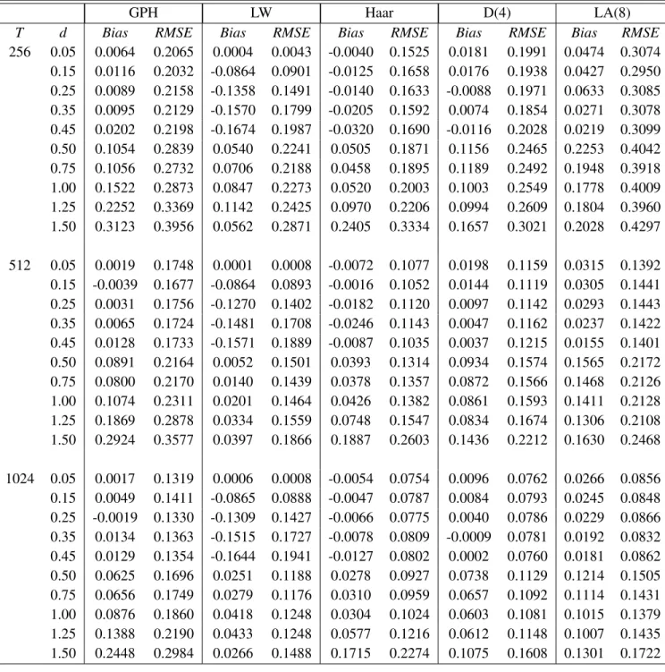
Table 6.4. Bias and RMSE of the GPH, LW and wavelet OLS estimator of the long memory

parameter for an ARFIMA(1,d,1),φ =0.2,θ =0.1

GPH LW Haar D(4) LA(8)

T d Bias RMSE Bias RMSE Bias RMSE Bias RMSE Bias RMSE

256 0.05 0.0064 0.2065 0.0004 0.0043 -0.0040 0.1525 0.0181 0.1991 0.0474 0.3074 0.15 0.0116 0.2032 -0.0864 0.0901 -0.0125 0.1658 0.0176 0.1938 0.0427 0.2950 0.25 0.0089 0.2158 -0.1358 0.1491 -0.0140 0.1633 -0.0088 0.1971 0.0633 0.3085 0.35 0.0095 0.2129 -0.1570 0.1799 -0.0205 0.1592 0.0074 0.1854 0.0271 0.3078 0.45 0.0202 0.2198 -0.1674 0.1987 -0.0320 0.1690 -0.0116 0.2028 0.0219 0.3099 0.50 0.1054 0.2839 0.0540 0.2241 0.0505 0.1871 0.1156 0.2465 0.2253 0.4042 0.75 0.1056 0.2732 0.0706 0.2188 0.0458 0.1895 0.1189 0.2492 0.1948 0.3918 1.00 0.1522 0.2873 0.0847 0.2273 0.0520 0.2003 0.1003 0.2549 0.1778 0.4009 1.25 0.2252 0.3369 0.1142 0.2425 0.0970 0.2206 0.0994 0.2609 0.1804 0.3960 1.50 0.3123 0.3956 0.0562 0.2871 0.2405 0.3334 0.1657 0.3021 0.2028 0.4297 512 0.05 0.0019 0.1748 0.0001 0.0008 -0.0072 0.1077 0.0198 0.1159 0.0315 0.1392 0.15 -0.0039 0.1677 -0.0864 0.0893 -0.0016 0.1052 0.0144 0.1119 0.0305 0.1441 0.25 0.0031 0.1756 -0.1270 0.1402 -0.0182 0.1120 0.0097 0.1142 0.0293 0.1443 0.35 0.0065 0.1724 -0.1481 0.1708 -0.0246 0.1143 0.0047 0.1162 0.0237 0.1422 0.45 0.0128 0.1733 -0.1571 0.1889 -0.0087 0.1035 0.0037 0.1215 0.0155 0.1401 0.50 0.0891 0.2164 0.0052 0.1501 0.0393 0.1314 0.0934 0.1574 0.1565 0.2172 0.75 0.0800 0.2170 0.0140 0.1439 0.0378 0.1357 0.0872 0.1566 0.1468 0.2126 1.00 0.1074 0.2311 0.0201 0.1464 0.0426 0.1382 0.0861 0.1593 0.1411 0.2128 1.25 0.1869 0.2878 0.0334 0.1559 0.0748 0.1547 0.0834 0.1674 0.1306 0.2108 1.50 0.2924 0.3577 0.0397 0.1866 0.1887 0.2603 0.1436 0.2212 0.1630 0.2468 1024 0.05 0.0017 0.1319 0.0006 0.0008 -0.0054 0.0754 0.0096 0.0762 0.0266 0.0856 0.15 0.0049 0.1411 -0.0865 0.0888 -0.0047 0.0787 0.0084 0.0793 0.0245 0.0848 0.25 -0.0019 0.1330 -0.1309 0.1427 -0.0066 0.0775 0.0040 0.0786 0.0229 0.0866 0.35 0.0134 0.1363 -0.1515 0.1727 -0.0078 0.0809 -0.0009 0.0781 0.0192 0.0832 0.45 0.0129 0.1354 -0.1644 0.1941 -0.0127 0.0802 0.0002 0.0760 0.0181 0.0862 0.50 0.0625 0.1696 0.0251 0.1188 0.0278 0.0927 0.0738 0.1129 0.1214 0.1505 0.75 0.0656 0.1749 0.0279 0.1176 0.0310 0.0959 0.0657 0.1092 0.1114 0.1431 1.00 0.0876 0.1860 0.0418 0.1248 0.0304 0.1024 0.0603 0.1081 0.1015 0.1379 1.25 0.1388 0.2190 0.0433 0.1248 0.0577 0.1216 0.0612 0.1148 0.1007 0.1435 1.50 0.2448 0.2984 0.0266 0.1488 0.1715 0.2274 0.1075 0.1608 0.1301 0.1722

1990 to January 29, 2010. The data are from the U.S. Energy Information Administration.19 We

consider a weekly nominal percentage return for crude oil series, i.e., rt =ln(Pt/Pt−1)∗100 for

t=1,2, . . . ,T, wherertis the return for crude oils at timet,Pt is the weekly current price andPt−1

19_{http://tonto.eia.doe.gov/dnav/pet/pet_pri_spt_s1_w.htm}

is the previous week’s price.

In the literature, the oil price has been analyzed by many authors, see for example Chang and Wong (2003) for oil price fluctuations in Singapore economy, Sadorsky (2006) for forecasting and modeling petroleum volatility, Lardic and Mignon (2006), Lardic and Mignon (2008) for oil prices and economic activities, Chen and Chen (2007) for financial assets, Narayan and Narayan (2007) for modeling and forecasting crude oil market volatility and Kang et al. (2009) for forecasting volatility of daily crude oil markets.

Figure (7.1) shows the dynamics of crude oil spot prices and return oil price of the two sample WTI

20 _{and Europe Brent}21 _{and figure (7.2) depicts a plot of volatility (i.e. of the absolute returns|r}

t|)

for the two crude oils and corresponding correlogram and spectrum function. We observe a slow decay of correlogram indicating the long memory behavior of the volatility of the weekly energy price.

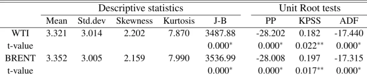
Table 7.1. Summary statistics and Unit Root tests of energy price volatility.

Descriptive statistics Unit Root tests

Mean Std.dev Skewness Kurtosis J-B PP KPSS ADF WTI 3.321 3.014 2.202 7.870 3487.88 -28.202 0.182 -17.440 t-value 0.000∗ 0.000∗ 0.022∗∗ 0.000∗ BRENT 3.352 3.005 2.159 7.990 3536.99 -28.008 0.197 -17.315

t-value 0.000∗ 0.000∗ 0.017∗∗ 0.000∗

Notes: Sample period, weekly data: Juin 15, 1990 to January 29, 2010. J-B is the Jarque-Bera statistic for null hypothesis of normality in sample volatility distribution. PP and ADF are the Phillips-Perron and

Augmented-Dickey-Fuller adjustedt-statistics of lagged dependent variable in a regression with intercept

and trend (H0: Data are I(1)). KPSS is the Kiwatkoski et al. (1992) test statistic based on residuals from

regression with intercept and trend (H0: Data are I(0)). The critical values for PP, KPSS and ADF are

−3.43, 0.216 and−3.96, respectively, at 1% significance level. * and ** indicate significance at 1% and

5% level, respectively.

Table(7.1) displays descriptive statistics and unit root tests of weekly volatility for both WTI and Brent crude oil spot prices. The sample mean and variance of volatility are around 3 and skewness and kurtosis statistics indicate that the volatility distribution is not normally distributed.

We apply three standard unit root tests on each individual transformed series, PP (Phillips-Perron), KPSS (Kwiatkoski, Phillips, Schmidt and Shin) and Augmented-Dickey-Fuller in order to show the stationarity behavior for weekly crude oil data. Results are given in table (7.1). For the PP and ADF tests, large negative values for the statistics support the rejection of the null hypothesis of unit root at the 1% significance level. For KPSS test, the statistics are significant at 5% level implying

20_{West Texas Intermidiate or Texas light Sweet is a type of crude oil used in the pricing of US domestic crudes, as}

well as oil imports into the US.

21_{Brent crude or Brent petroleum is used as a reference for pricing a number of other crude streams. It is produced}

in North sea region.

Figure 7.1. Oil price time series. 0 200 400 600 800 1000 20 40 60 80 100 120 140 Pr ice ($/Barrel) WTI 0 200 400 600 800 1000 −20 −10 0 10 20 Retur ns (%) 0 200 400 600 800 1000 20 40 60 80 100 120 140 Pr ice ($/Barrel) BRENT 0 200 400 600 800 1000 −20 −10 0 10 20 Retur ns (%)

Notes: Level and return oil price in the period between Jun 15, 1990 and January 29, 2010.

that the two series are stationary models. Hence, the volatility crude oil price series are stationary. Thus, we can examine evidence for any possible long-range dependence phenomenon.

To implement the tapering on non stationarity crude oil data, we have concentrated on the Bartlett

and Zhurbenko Kolmogorov tapers. We plotted these data tapers for p=2 and p=3 for sample

size T =1024 on the first row of Fig. 7.3. The tapered crude oil series h_tp_t are plotted in the

second and fourth rows. In the third and fifth rows of the pictures we plotted the log-periodogram of tapered crude oil series.

7.2. Long memory of crude oil spot price volatility

Baillie et al. (1996), introduced the Fractionally Integrated GARCH (FIGARCH) model as gen-eralization of the GARCH and Integrated GARCH (IGARCH) specifications, see Beine et al. (2002), Giraitis et al. (2004), Lardic and Mignon (2004), Lee (2005) and Baillie et al. (2007) for a few recent applications. They suggested the FIGARCH model because is able to distinguish between short and long memory in conditional variance behavior. Let the conditional variance

ht=Var(εt|Ωt−1)whereΩt−1is the information set in periodt−1. The GARCH model is written

Figure 7.2. Energy price analysis. 0 200 400 600 800 1000 0 5 10 15 20 25 WTI V olatility 0 200 400 600 800 1000 0 5 10 15 20 BRENT V olatility 5 10 15 20 −0.05 0.00 0.05 0.10 0.15 0.20 0.25 Lag A CF WTI 5 10 15 20 −0.05 0.00 0.05 0.10 0.15 0.20 Lag A CF BRENT 0.0 0.1 0.2 0.3 0.4 0.5 2 5 10 20 frequency spectr um WTI bandwidth = 0.00189 0.0 0.1 0.2 0.3 0.4 0.5 2 5 10 20 50 frequency spectr um BRENT bandwidth = 0.00189

Notes: weekly volatility WTI (top left) and Brent (top right) crude oil spot price in the period Jun 15, 1990 to January 29, 2010 and corresponding ACF and spectrum function.

as

(1−β(L))ht=ω+α(L)εt2. (7.1)

where β(L) and α(L) are polynomials of order p and q, respectively. Let νt =εt2−ht. The

FIGARCH model is defined as follows:

φ(L) (1−L)dε_t2=ω+ (1−β(L))νt. (7.2)

whereφ(L) = [1−β(L)−α(L)] (1−L)−d. Note that the FIGARCH model reduces to a GARCH

model whend=0 and to an IGARCH model whend=1. The conditional variance of FIGARCH

model may be written as

ht= ω 1−β(L)+λ(L)ε 2 t. (7.3) Whereλ(L) =1− φ(L)(1−L)d/[1−β(L)].

In our analysis, we first estimate the fractional integration parameter d by the three methods

de-scribed previously in section 5. The estimates results are provided in table (7.2). These estimates indicate evidence of long memory in WTI and Brent crude oil volatility.

We also assess the null hypothesis of a White noise model for WTI and Brent returns using

Box-Pierce test statisticsQ(24). The corresponding t-statistics are 70.722 and 69.397 for WTI and Brent

returns, with p−value=0, respectively. Thus, we find significant evidence of serial dependence

in the volatility series. Therefore, this finding implies non-normality and serial correlation in the crude oil volatilities. We used a filter to remove the serial dependence in the return series and the resulting residuals series are re-tested for GARCH and FIGARCH models to detect the long memory phenomenon in the volatility of crude oils spot prices. We used an autoregressive moving average ARMA(p,q) model to take out all the linearity in the return series. The identification of the

autoregressive and moving average orders pand qare based on the lowest AIC. The Box-Pierce

Q-statistics (not presented here) showed that the residuals of an ARMA(3,3) and ARMA(3,1) are White noise for the WTI and Brent return, respectively.

Second, we reported the estimation results of the GARCH and FIGARCH models in table (7.4). We showed that the FIGARCH (1,d,1) describe volatility persistence for the two crude oil prices.

The estimates of long memory parameterd are 0.72 and 0.94 for the WTI and Brent, respectively,

rejecting the null hypothesis of the GARCH model (d=0). This result indicates persistence in the

conditional variance of the volatility crude oils. Therefore, the FIGARCH model is able to capture persistence in the volatility of crude oils.

Table 7.2. GPH, LW and wavelet OLS estimates. WTI Brent p=1 p=2 p=3 p=1 p=2 p=3 Panel A: GPH (1983) Spot price (pt) 0.904 (0.000) 1(0..142000) 1(0..187000) 0(0..864000) 1(0..117000) 1(0..122000) return (rt) −0.144 (0.282) 0.019 (0.984) 0(0..082934) −0.181 (0.177) −0.001 (0.998) 0.075 (0.940) Absolute return (|rt|) 0.379 (0.004) 0(0..542000) 0(0..515000) 0(0..395003) 0(0..623000) 0(0..626000)

Panel B: Local Whittle

Spot price (pt) 1.008 (0.000) 0(0..925000) 0(0..857000) 1(0..008000) 0(0..971000) 0(0..832000) return (rt) 0.027 (0.079) 0(0..021172) 0(0..027079) 0(0..006658) 0(0..004757) −0.002 (0.876) Absolute return (|rt|) 0.623 (0.000) 0 .374 (0.000) 0 .347 (0.000) 0 .518 (0.000) 0 .299 (0.000) 0 .223 (0.000)

Panel C: Haar filter

Spot price (pt) 0.854 (0.001) 1(0..558000) 1(0..541000) 0(0..826001) 1(0..510000) 1(0..497000) return (rt) −0.055 (0.000) 0.033 (0.000) 0(0..046000) −(00..000030) 0.023 (0.000) 0(0..032000) Absolute return (|rt|) 0.137 (0.000) 0(0..207001) 0(0..227002) 0(0..114000) 0(0..208000) 0(0..229000) Panel D: D(4) filter Spot price (pt) 0.608 (0.001) 1(0..318000) 1(0..359000) 0 .636 (0.002) 1(0..318000) 1(0..344000) return (rt) −0.117 (0.000) −0.019 (0.000) −0.003 (0.001) −0.126 (0.008) −0.040 (0.006) −0.026 (0.005) Absolute return (|rt|) 0.159 (0.004) 0(0..195004) 0(0..190004) 0(0..087003) 0(0..171004) 0(0..180005)

Panel E: LA(8) filter

Spot price (pt) 0.529 (0.012) 1(0..324005) 1(0..400001) 0(0..571016) 1(0..328007) 1(0..398005) return (rt) −0.070 (0.004) 0.031 (0.007) 0(0..047008) −0.006 (0.036) 0.076 (0.043) 0(0..089040) Absolute return (|rt|) 0.069 (0.025) 0(0..139027) 0(0..144031) −0.018 (0.001) 0.092 (0.011) 0(0..196014)

Notes:(pt),(rt)and|rt|are, respectively, crude oil spot price, return and absolute return. The value

between parentheses are p-values. p=1,2 and 3 are the orders of the taper. p=1 means no tapering, p=2 is the Bartlett taper and p=3 is the Zhurbenko Kolmogorov taper.

Table 7.3. ARMA model estimation for the oil price returns. ˆ φ0 φˆ1 φˆ2 φˆ3 θˆ1 θˆ2 θˆ3 WTI 0.1420 (0.1563) 0(0..27670312) −0.5153 (0.0278) −0.2293 (0.0318) −0.1677 (0.3456) 0.4134 (0.00) 0(0.4273.1488) BRENT 0.1527 (0.1819) −0.3251 (0.0312) 0.0893 (0.0484) 0(0..09880323) 0(0.5041.2603)

Notes: The value between parentheses are standard deviation. he mean µ was clearly

non-signicant for the tow processes.

Figure 7.3. Data tapers, tapered oil series and log-periodogram of tapered series. 0 200 400 600 800 1000 0.0 0.2 0.4 0.6 0.8 1.0 p=2 time h(t) 0 200 400 600 800 1000 0.0 0.2 0.4 0.6 0.8 1.0 p=3 time h(t) 0 200 400 600 800 1000 0 5 10 15 20 25 30 35 WTI time p(t).h(t) 0 200 400 600 800 1000 0 5 10 15 20 25 30 35 WTI time p(t).h(t) 0.0 0.1 0.2 0.3 0.4 0.5 −30 −20 −10 0 10 20 30 40 WTI bandwidth = 0.000282, 95% C.I. is (−6.26,16.36)dB frequency log−P er iodogr am 0.0 0.1 0.2 0.3 0.4 0.5 −40 −20 0 20 40 WTI bandwidth = 0.000282, 95% C.I. is (−6.26,16.36)dB frequency log−P er iodogr am 0 200 400 600 800 1000 0 5 10 15 20 25 30 35 Brent time p(t).h(t) 0 200 400 600 800 1000 0 10 20 30 Brent time p(t).h(t) 0.0 0.1 0.2 0.3 0.4 0.5 −30 −20 −10 0 10 20 30 40 Brent bandwidth = 0.000282, 95% C.I. is (−6.26,16.36)dB frequency log−P er iodogr am 0.0 0.1 0.2 0.3 0.4 0.5 −40 −20 0 20 40 Brent bandwidth = 0.000282, 95% C.I. is (−6.26,16.36)dB frequency log−P er iodogr am

Notes: The columns correspond to data tapers of orders p=2,3, respectively.

In the first row, the plots correspond to the weightsht. In second and fourth

rows we plot the tapered series htpt. In the third and fifth rows appear the

log-periodogram of the above series plotted against frequency.

Table 7.4. Estimation results for Crude oil price

WTI BRENT

GARCH FIGARCH GARCH FIGARCH

ω 0.6866 (0.004) 0(.03758.022) 0(.04427.020) 0(.02549.017) α 0.0.091 (0.000) 0(.00945.000) β 0.871 (0.000) 0(.07941.000) 0(.08843.000) 0(.08732.000) Qs(24) 25.621 (0.372) 26(0..331434) 26(0..324575) 26(0.3098.884) d-FIGARCH 0.7262 (0.000) 0(.09477.000) φ 0.1888 (0.000) 0(.00286.850) Notes: p-values are in parentheses below corresponding parameter

esti-mates.Qs(24)is the Box-Pierce test statistic for lag 24.

8. Conclusion

In this paper we considered a simulation study to evaluate the procedure for estimating the long memory parameter in stationary and non stationary time series. We have compared three

semipara-metric methods for the estimation of the fractional parameter d in four models: ARFIMA(0,d,0),

ARFIMA(1,d,0), ARFIMA(0,d,1) and ARFIMA(1,d,1). These estimates are the Geweke and Porter-Haduk (1983), the Local Whittle (Robinson, 1995b) and the wavelet Ordinary Least-Square (Jensen,

1999). We have used the Bartlett and Zhurbenko Kolmogorov tapers with orders p=2 and p=3,

respectively, in non stationary models. According to the simulation results we have showed that the

order pof taper has a strong impact on the performance of estimates. Ford≤0.25 and ford≥1.5

the Local Whittle estimate possesses a small mean squared error than the GPH and wavelet OLS estimates for small and large sample sizes and for different values of long memory parameter. But,

ford ∈[0.25,1.5)the performance of Haar estimate (Jensen, 1999) usually is better than the two

other estimates.

The estimation results showed that the volatility of crude oil prices exhibit strong evidence of long memory which can be captured by FIGARCH model.

References

Abry, P., Veitch, D. (1996). Wavelet analysis of long-range-dependence traffic. IEEE Transactions

on Information Theory. 44, 2–15.

Baillie, R.T., Bollerslev, T. and Mikkelsen, H.O. (1996). Fractionally integrated generalized

au-toregressive conditional heteroskedasticity. Journal of Econometrics. 74, 3–30.

Baillie, R.T., Han Y.W., Myers, R.J. and Song, J. (2007). Long memory and FIGARCH models for

daily and high frequency commodity prices. Journal of Futures Markets. 27, 643-668.

Beine, M., Laurent, S. and Lecourt C. (2002). Accounting for conditional leptokurtosis and closing

days effects in FIGARCH models of daily exchange rates. Applied Financial Economics. 12,

589-600.

Beran, J. (1994). Statistics for long memory processes. New York: (Chapman & Hall).

Bollerslev, T. and Mikkelsen, H. O. (1996). Modeling and pricing long memory in stock market

volatility. Journal of Econometrics. 73, 151-184.

Boutahar, M., Marimoutou, V. and Nouira, L. (2007). Estimation Methods of the Long Memory

Parameter: Monte Carlo Analysis and Application. Journal of Applied Statistics. 34, 261-301.

Brillinger, D. R. (1981). Time Series: Data analysis and Theory. Expanded Edition, 540 pp.,

Holden-Day. San Francisco, CA.

Chang, Y., Wong, J.F. (2003). Oil price fluctuations and Singapore economy. Energy Policy. 31,

1151-1165.

Chen, W. W. (2001). Tapering and nonstationarity/non invertibility in time series. Presented at Symposium on New Directions in Time Series Analysis, CIRM, Luminy, France.

Chen, G., Abraham, B. and Peiris, S. (1994). Lag window estimation of the degree of differencing

in fractionally integrated time series models. Journal of Time Series Analysis. 15, 473–487.

Chen, S.S. and Chen, H.C. (2007). Oil prices and real exchange rates. Energy Economics. 29,

390-404.

Crato, N. and de Lima, P. J. F. (1994). Long range dependence in the conditional variance of stock

returns. Economics Letters. 45, 281-285.

Dahlhaus, R. (1989). Efficient parameter estimation for self-similar processes. The Annals of

Statistics. 17, 1749-1766.

Daubechies, I. (1992). Ten Lectures on Wavelets. CBMS-NSF Series in Applied Mathematics. 61.

SIAM, Philadelphia.

Davidson, R., Labys, W.C. and Lessourd, J.B. (1998). Wavelet Analysis of Commodity Price

Behavior. Computational Economics. 11, 103-128.

Dickey, D. and Fuller, W. (1979). Distribution of the estimators for autoregressive time series with

unit root. Journal of the American Statistical Association. 74, 427-431.

Diebold, F. X. and Rudebush. G. (1989). Long memory and persistence in aggregate output.

Journal of Monetary Economics.24, 189-209.

Faÿ, G., Moulines, E., Roueff, F. and Taqqu, M.S. (2009). Estimators of long-memory: Fourier

versus wavelets. Journal of Econometrics. 151, 159-177.