04 August 2020
POLITECNICO DI TORINO
Repository ISTITUZIONALE
Satellite Image Segmentation with Deep Residual Architectures for Time-Critical Applications / Ghassemi, Sina; Sandu, Constantin; Fiandrotti, Attilio; Tonolo, Fabio Giulio; Boccardo, Piero; Francini, Gianluca; Magli, Enrico. - (2018), pp. 2235-2239. ((Intervento presentato al convegno European Signal Processing Conference tenutosi a Rome, Italy nel Sep. 2018.
Original
Satellite Image Segmentation with Deep Residual Architectures for Time-Critical Applications
Publisher: Published DOI:10.23919/EUSIPCO.2018.8553545 Terms of use: openAccess Publisher copyright
(Article begins on next page)
This article is made available under terms and conditions as specified in the corresponding bibliographic description in the repository
Availability:
This version is available at: 11583/2721854 since: 2019-03-14T11:34:07Z
Satellite Image Segmentation with Deep Residual
Architectures for Time-Critical Applications
Sina Ghassemi
∗, Constantin Sandu
‡, Attilio Fiandrotti
∗, Fabio Giulio Tonolo
‡, Piero Boccardo
†, Gianluca Francini
§and Enrico Magli
∗∗Dept. of Electronics and Telecommunications, Politecnico di Torino, Turin, Italy [sina.ghassemi—attilio.fiandrotti—enrico.magli]@polito.it
†Dept. of Regional and Urban Studies and Planning, Politecnico di Torino, Turin, Italy, [email protected] ‡ITHACA, Information Technology for Humanitarian Assistance, Cooperation and Action, Turin, Italy
[constantin.sandu—fabio.giuliotonolo]@ithaca.polito.it
§Telecom Italia S.p.A., Torino, Italy, [email protected]
Abstract—This work addresses the problem of training a convolutional neural network for segmenting satellite images in emergency situations, where images to be segmented are potentially very different from training images. Such case is particularly challenging due to the large intra-class variations in image statistics between images captured at different locations by different sensors. We propose a convolutional encoder-decoder network architecture where the encoder is built around residual networks. We show that the proposed architecture enable learn-ing features able to generalize the learnlearn-ing process across images with largely different statistics. Our architecture can accurately segment images that have no reference in the training set, whereas a minimal refinement of the trained network significantly boosts the segmentation accuracy.
I. INTRODUCTION
Hand-segmenting satellite images is a labor-intensive pro-cess, thus fast, reliable schemes for automatic satellite image segmentation are desirable. Image segmentation can be defined as the problem of classifying each pixel in an image according to a number of (predefined) labels. Most of the existing schemes for satellite image segmentation [1] deal with the case where training samples are first extracted from part of the image, then a supervised algorithm is trained to segment the rest of the same image. This work addresses the particular yet important case of training an algorithm so that it can be quickly deployed over images that differ substantially from the training samples. This is the case of satellite based emergency map-ping, when a large number of image interpreters is required to manually carry out reference mapping and damage assessment analyses in a short time frame (few hours) [2]. The challenging aspect of such applications is the potentially large intra-class statistics variations between training and deployment images, which requires a highly-generalized learning process.
Convolutional Neural Networks (CNNs) recently outper-formed many competing techniques in a number of image processing tasks [3], [4]. First a number ofconvolutionallayers extracts discriminative features of increasing semantic level from the the input image. Position (and scale) robustness are achieved discarding absolute spatial information via repeated convolve-and-subsample operations. Considering a classic
im-age classification problem, one or morefully connectedlayers label the entire image among a finite set of options accord-ing to such features. Notably, CNNs can be trained end-to-end to learn such features, avoiding handcrafting the feature extractor [5]. However, subsampling operations and fully con-nected layers remove most of the spatial information, making classification-tailored CNNs unsuited for image segmentation.
Fully convolutionalCNNs (FCNs) recently showed promis-ing results in image segmentation [6]. In a FCN, deconvolu-tional[7] layers are used to reverse the subsampling process, upsampling feature maps and recovering the spatial resolution. Then, unitary-sized convolutional filters replace the fully con-nected layers preserving feature position. Symmetric encoder-decoder architectures and aggressive augmentation help further performance [8]. In addition, conditional random fields based postprocessing may further refine the segmentation accuracy by leveraging context information [9]. FCN-based architec-tures recently achieved state of the art performance in the ISPRS segmentation competition [10], [11].
This work investigates architectures [4] for satellite image segmentation. We propose an encoder-decoder CNN architec-ture with a residual encoder and deconvolutional decoder that can be trained in a fully-supervised manner. We experiment with residual networks of different depth, training the net-work over images vastly different from deployment images. Experiments show that network depth improves segmentation performance. Most important, residual networks enable the deep architectures required to learn features good enough to generalize across images with statistics largely different from training images. Moreover, we show that refining the trained network over a small hand-annotated portion of the deploy-ment images can dramatically boosts the network performance with little extra effort.
The rest of this paper is organized as follows. Sec. II provides the background relevant to this work. Sec. III de-scribes the proposed network architecture and relative training procedures. Sec. IV describes the experimental methodology and relative results. Conclusions are drawn in Sec. V.
II. BACKGROUND
A. Residual Networks
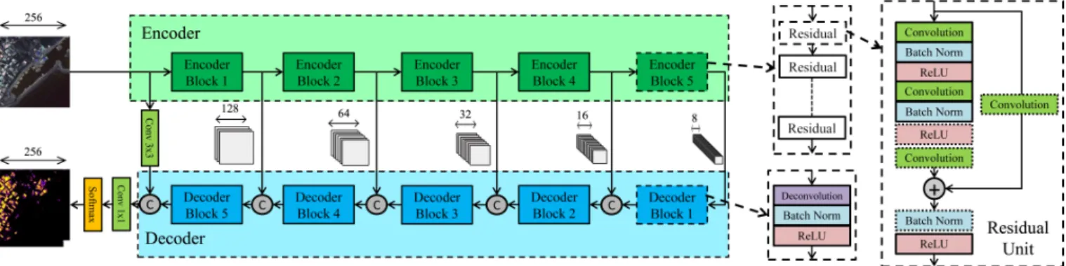
Residual Networks (ResNets) [4] are a class of CNNs that enable deep topologies while maintaining the number of learnable parameters under control. We refer to the basic block of a ResNet asunitin the following. Each unit includes two or three convolutional layers with 3×3 or 1×1 filters and ReLU activation functions as illustrated in Fig. 1 (right box). The output of the last convolutional layer is added with the input of the first layer via a skip connection. Multiple residual units are stacked without intermediate pooling operators to create a residual block. Notice that the filters in the first convolutional layer of each block have stride equal to two to compensate for the lack of pooling operators. The number and the size of the feature maps within each block is homogeneous, and multiple blocks can be stacked to create very deep topologies. Concerning image classification applications, the last block of a ResNet is typically followed by a pooling operator and a fully connected layer with C neurons, one per each classification label. The supervised training of a ResNet is equivalent to learning one residual function for each unit, which makes ResNets easier to train than conventional CNNs of identical depth.
B. Deconvolutional Networks
Deconvolutional networks were introduced as an unsuper-vised framework for coping with the loss of mid-level cues [7] due to pooling operations. In our image segmentation framework, we leverage deconvolutional layers as a supervised method for spatially upsampling feature maps in the decoder. Each deconvolutional layer (backward convolution) performs two operations. First, the input feature map is spatially up-sampled (unpooling) by a two factor padding missing features with zero value features. Second, such sparse feature map is convolved with a number of filters which learn how to recover the missing features. Such operation generates a dense output feature map which is upsampled by a two factor with respect to the input feature map. Therefore, deconvolutional layers can be approximated as learnable upsampling filters that we exploit to increase the spatial resolution of segmented images.
III. PROPOSEDARCHITECTURE
A. Network Architecture
The overall convolutional network architecture we propose is illustrated in Fig. 1 and it consists of an encoder sub-network responsible for feature extraction followed by a
decodersub-network responsible for spatial resolution restora-tion and image segmentarestora-tion ultimately [8].
1) Encoder: The encoder subnetwork takes as input a image sized 256×256 composed of D spectral channels. The encoder sub-network is composed of five residual blocks as follows. As an exception to the ResNet architecture, the first block includes one single convolutional layer with 7×7 filters and 2 pixel stride, followed by a 2 × 2 pooling layer. All other blocks include a variable number of residual units for
learning features of increasing semantic depth and decreasing spatial resolution. The number of feature maps produced in output by each block is strictly twice the number of feature maps generated by the previous block. However, filters in the first convolutional layer of each block have a stride equal to 2 pixels and halve the feature maps edge size, keeping the number of features under control. So, the receptive field size of each feature map increases at each block depending on the number of convolutional layers in the units. Increased receptive fields enable the network to correlate pixels over larger and larger spatial contexts. At the end, encoder outputs a certain number of feature maps which can be seen as coarse 8×8 representation of the input image. Using residual network as encoder enables us to use larger number of convolutions in encoder compare to other types of convolutional networks such as Inception [3].
2) Decoder: The decoder sub-network is composed by a sequence of five deconvolutional blocks which recover the spatial resolution lost at the encoder due to pooling and subsampling. Each deconvolutional block is composed by a deconvolutional layer [7] with 4×4 filters and 2 pixel stride and ReLU activation functions with batch normalization. Each deconvolutional block learns the features required to produce a reduced number of upsampled feature maps with respect to the input feature maps in input. For example, the first decon-volutional block takes in input the 512 8 × 8 feature maps generated by the last block of the encoder and produces 256 16 ×16 feature maps effectively doubling the overall number of features and recovering spatial information. As Fig. 1 shows, Feature maps generated by each deconvolutional block are concatenated with an equal number of identically sized feature maps generated by the matching encoder block [12]. We verified that best performance is obtained when the number of downsampled (encoder) and upsampled (decoder) feature maps is balanced. Balanced feature maps concatenation, we understand, avoids that any of the two types of features dominate the other when fed to subsequent deconvolutional blocks. Further deconvolutional blocks further increase the feature maps resolution while reducing their overall count. The fifth deconvolutional block finally generates 64 feature maps sized 256×256, recovering the original image resolution. Our experiments also revealed that better performance is achieved when such feature maps are concatenated with an identical number of identically sized feature maps generated by 3 × 3 filters. Finally, the (upsampled) feature maps are convolved with 1×1 filters [6] so to generate a number of output feature maps equal to the number of classesC. Thei-th feature in the
k-th output feature mapoi,krepresents the relative confidence
that thei-th pixel in the input image belongs to thek-th class. However, we are interested in estimating, for eachi-th pixel, the pixel class probability distribution over thekclassesyi,k.
To this end, spatial SoftMax is used as partition function to produce the sought scoreyi,k =eoi,k/P
C k=1e
oi,j, such that
PC
k=1yi,k= 1.
Table I summarizes the hyperparameters for some common ResNet variants used in proposed network.
Fig. 1: Proposed encoder-decoder network architecture for satellite image segmentation with exploded residual block and unit diagram and deconvolutional blocks.
TABLE I: Number of (output feature maps, convolutional layers) for each encoder (top) and decoder (bottom) block.
Encoder Num. of (feature maps, convolutions) in encoder block depth Block 1 Block 2 Block 3 Block 4 Block 5
18 (64, 1) (64, 4) (128, 4) (256, 4) (512, 4) 34 ” (64, 6) (128, 8) (256, 12) (512, 6) 50 ” (256, 9) (512, 12) (1024, 18) (2048, 9) 101 ” ” ” (1024, 69) ” 152 ” ” (512, 24) (1024, 108) ” 200 ” ” (512, 72) ” ” Encoder Num. of (feature maps, convolutions) in decoder block
depth Block 1 Block 2 Block 3 Block 4 Block 5 18,34 (256, 1) (128, 1) (64, 1) (64, 1) (64, 1)
>34 (1024, 1) (512, 1) (256, 1) ” ”
B. Training Samples Generation
Our network is trained over images where each pixel is labeled according to one out ofCpossible classes. First, every image is subdivided in tiles of 364 ×364 pixels each with a stride of 120 pixels (tiles overlap by 244 pixels horizontally and vertically). For each image, 80% of the tiles are used for extracting training samples, whereas the remaining 20% are reserved for validation samples (training and validation areas are disjoint sets).
Concerning training samples, a number of random transforma-tions are performed on each tile. First, with 50% probability, we crop a 256×256 patch at a random location from the tile, matching our proposed network input window size. Otherwise, the tile is first randomly rotated by θ∈(0,2π)degrees, then a 256×256 sample is cropped from the tile center. Next, the sample is randomly flipped horizontally and vertically with 50% probability respectively.
Such transformations are independently performed over each training tile at each training epoch and are pivotal to augment [8] the number of unique samples shown to the network during training, preventing the network from overfitting to the train data. Notice we experimented with additional random variations in illumination and contrast variations and with random color jittering, however with marginal gains only. Concerning validation tiles, we simply extract a 256 × 256 patch from the center of each tile.
The samples are then normalized with respect to mean pixel intensity value and standard deviation. For each channel, we subtract from each pixel intensity value the mean intensity value and divide by the standard deviation. Normalization significantly accelerates the learning process and shall be applied also at deployment time.
C. Cost Function Definition
Training our network over sample xis equivalent to find-ing the set of network parameters (weights, biases) w that minimize some error(or loss) function L(w, y, t) wherey is the actual network output to xandt is the expected (target) network output. Let us indicate as ti,k the expected output
for thei-th pixelxi and for the k-th class amongCdifferent
possible classes. Let us assume thattitakes the form of a
one-hot vector, i.e. only the element corresponding to the correct class is equal to one, whereas all the other C−1 elements are equal to zero. The error functionL(w, y, t)represents the network inaccuracy in segmenting samplexand is defined as
L(w, y, t) =− H×W X i=1 C X k=1
ti,k log (yi,k). (1)
That is, the segmentation error is defined as the sum of teh cross-entropy between yi and ti for every i-th pixel xi in
sample x.
It is obviously desirable that the network learns to segment also samples it has never seen at training time. To this end, thecost function we actually optimize at training time is
J(w, y, t) =ηL(w, y, t) +λR(w), (2) whereR(w)is a regularization term defined as the squared L2 norm of all the weights in the network. That is, we minimize a cost function that is a linear combination of a loss function (pixel classification error) and a regularization term, whose weight is controlled by the parameters η (learning rate) and
λrespectively.
D. Training Procedure
Finally, we proceed training the network by finding a set of network parameters w that minimize the cost function in
Eq. (2). First, the derivatives of the cost function J(w, y, t) with respect to parameters w are recursively computed via backpropagation [5] for each training samplex. Parametersw
are updated via stochastic gradient descent with momentum and over minibatches of B training samples each. Batch training allows higher learning rates and in general lower training and validation errors. Notice that the upper limit to
B depends on the amount of memory available at training time (derivatives of network parameters for all B training samples shall be kept in memory at the same time). With this respect, residual networks are the key towards larger batch sizes B as they entail fewer learnable parameters to hold in memory. Manually updating the learning rate η showed to somewhat improve the performance with respect to the widely used AdaGrad learning rate adaptation algorithm. The training ends when the cost function computed over the validation set stops decreasing.
IV. EXPERIMENTALRESULTS
A. Dataset
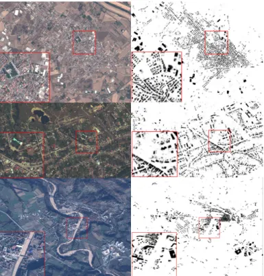
We experiment with a total of 9 very high resolution images acquired by three different Earth Observation (EO) satellites over 9 areas of interest worldwide. The images feature four spectral bands (blue, green, red and IR) with a nominal spatial resolution of 0.5 m and different off-nadir angles. We split the dataset into two subsets: 6 images (D5, D13, D16, D17, D18 and D20) are used for training and validation, whereas 3 images (D12, D19 and D22) are reserved for testing. Ground truth was generated exploiting OpenStreeMap data, and manually refined and completed where required. Valida-tion regions are extracted from the 6 training images to cover approximately 20 percent of each image area and statistically sample almost all types of texture present in the area. Training and validation regions are subdivided in tiles from which 256 × 256 samples are extracted as described in Sec. III-B. The 3 test images D12, D19 and D22 in Fig. 2 (left) are 6000 × 4500, 3700 × 2100 and 8700 × 6600 respectively. 512 ×512 tiles from each image are extracted and independently processed in a fully convolutional way to account for the GPU memory constraints of our experimental setup. Resulting maps are finally stitched together and overlapping maps regions are averaged where needed to avoid artifacts.
B. Testbed and Metrics
The network described in Sec. III-A is trained over the previously described dataset of satellite images as described in Sec. III-D. In detail, we use batches of B=8 samples, a momentum of 0.9 and initial learning rate of 0.005 that we divide by a 5 every 30 epochs. We experiment separating the buildings from the ground, i.e. our image segmentation network operates as a binary pixel classifier (C=2). The network is implemented using the Torch framework and is trained over an NVIDIA TitanX Pascal GPU with 12 GB of memory.
We evaluate the trained network using two metrics. First, the
F1 scoreis the harmonic mean of precision and recall and is
defined as F1 = 2· precisionprecision+·recallrecall, where precision is the fraction of correctly labeled pixels and recall is the fraction of correctly predicted positive (building) pixels. Finally,accuracy
is the overall fraction of correctly labeled to all pixels.
C. Results
Our first experiment addresses the deployment situation where it is not affordable at all to hand-annotate the image to be processed. Table II evaluates our proposed architecture with different ResNet-based encoder variants as in Table I. As a reference, we experiment with the standard U-Net [8] ar-chitecture (19 convolutional layers, comparable to ResNet18) and a deeper (35 layers, comparable to ResNet34) variant. Our proposed architecture consistently outperforms the U-Net reference for comparable network depths. The table also shows that the encoder depth plays a key role on the overall system performance, whereas increasing the encoder depth beyond 152 layers does not improve performance any further. This first experiment proves that encoder depth improves performance, however the proposed residual-based encoder yields better performance for comparable depth demonstrating better ability towards generalized learning. While Fig. 2 shows the segmentation result of Prop-152, due to page constraints, supplementary results are accessible via an external link1. TABLE II: Results over test areas in terms of f1 score and accuracy.
area D12 area D19 area D22 Mean F1 Acc. F1 Acc. F1 Acc. F1 Acc. U-Net(19) [8] 58.17 94.10 61.37 92.10 64.23 96.85 61.25 94.35 U-Net(35) 59.16 94.12 61.17 93.12 66.32 97.77 62.21 95.03 Prop-18 57.08 93.87 63.58 92.89 67.75 97.54 62.80 94.76 Prop-34 59.17 94.12 65.92 93.48 69.83 97.85 64.97 95.15 Prop-50 58.33 93.49 64.10 93.39 69.92 97.85 64.11 94.91 Prop-101 64.95 94.45 67.26 93.59 70.65 97.83 67.62 95.29 Prop-152 67.72 94.70 68.01 93.61 72.93 97.91 69.55 95.40 Prop-200 67.70 94.48 66.86 93.49 71.85 97.84 68.80 95.27
In the second experiment, we investigate refining the trained network over small regions of the test regions (removed for the purpose from the test set). This experiment addresses the deployment situation where it is affordable to hand-annotate a small portion of the image to be processed. To this end, we further train the 152 layers encoder network and also U-Net (19) with a learning rate equal to 10−4 for
100 epochs. We experiment refining the network over areas covering either about 7 percent (small) or 15 percent (large) of the region. The refined network is then evaluated over the rest of each test region. Table III shows consistent gains for all experimental setups with respect to the reference case where the network is trained over a totally distinct set of images with respect to the test set. This experiment shows that refining a pretrained network over a small annotated portion of the test area consistently improves the segmentation performance. Whereas the reference U-Net architecture benefits the most from refinement, that is because our proposed architecture performs already well without refinement, thus fine-tuning gains are smaller.
TABLE III: Comparison between non-refined and refined network architectures (U-Net and proposed).
area D12 area D19 area D22 Mean F1 Acc. F1 Acc. F1 Acc. F1 Acc. Prop-152 67.72 94.70 68.01 93.61 72.93 97.91 69.55 95.40 Tuned 70.46 94.77 71.18 94.15 75.80 98.03 72.48 95.65 (small) +2.74 +0.07 +3.17 +0.54 +3.33 +0.02 +3.08 +0.21 Tuned 74.70 95.40 73.40 94.16 77.24 98.24 75.11 95.93 (large) +6.98 +0.70 +5.39 +0.55 +4.31 +0.33 +5.56 +0.52 U-Net 58.17 94.10 61.37 92.10 64.23 96.85 61.25 94.35 Tuned 67.70 94.46 68.97 93.95 64.40 96.87 67.02 95.09 (small) +9.53 +0.36 +7.60 +1.85 +0.17 +0.02 +5.77 +0.74 Tuned 73.90 95.48 71.78 94.13 73.10 97.91 72.72 95.84 (large) +15.73 +1.38 +10.34 +2.03 +8.87 +1.06 +11.47 +1.49
Furthermore, we experimented postprocessing the seg-mented images via Conditional Random Fields(CRF). Namely, CRF refines the segmentation by minimizing an energy func-tion based on pixel values in input image and the network output. Our experiments showed minor improvements only: we attribute that to the fact that in our test images the boundaries between areas are not always sharp, and furthermore the generated segmentation map had already been refined by the decoder subnetwork with skip connections.
Concerning segmentation time, a critical factor in emer-gency mapping, processing each of the three test images took 110, 55 and 200 seconds for images D12, D19 and D22 respectively. Finally, the extra training time required for refinement amounts to about 2 hours per image in our setup (by comparison, manually annotating the test images required about 10 hours each).
V. CONCLUSIONS
We proposed an encoder-decoder convolutional neural net-work that practically enables time consuming satellite imagery processing steps crucial for emergency mapping. The encoder is based on a deep residual design, on the assumption that residual networks are capable of generalizing the learning process as required in emergency mapping that can be used worldwide in areas where no reference data are available. Our experiments prove our assumptions, demonstrating that segmentation accuracy improves with the encoder depth. Moreover, the residual design allows deeper encoders and larger batch sizes in reason of the lower number of learnable parameters. Finally, fine-tuning a pretrained network over small annotated area of the image to be processed further boost the performance for minimal additional complexity. Future tests will address also the post-event satellite image analyses, focusing on damage assessment tasks.
REFERENCES
[1] Liangpei Zhang, Lefei Zhang, and Bo Du, “Deep learning for remote sensing data: A technical tutorial on the state of the art,” IEEE Geoscience and Remote Sensing Magazine, vol. 4, no. 2, pp. 22–40, 2016.
[2] Stefan Voigt, Fabio Giulio-Tonolo, Josh Lyons, Jan Kuˇcera, Brenda Jones, Tobias Schneiderhan, Gabriel Platzeck, Kazuya Kaku, Manzul Kumar Hazarika, Lorant Czaran, et al., “Global trends in satellite-based emergency mapping,” Science, vol. 353, no. 6296, pp. 247–252, 2016.
Fig. 2: Test images D12 (top), D19 (middle), D22 (bottom) on the left and corresponding segmentation on the right. Detail of the segmented image in the red box.
[3] Christian Szegedy, Wei Liu, Yangqing Jia, Pierre Sermanet, Scott Reed, Dragomir Anguelov, Dumitru Erhan, Vincent Vanhoucke, Andrew Rabinovich, et al., “Going deeper with convolutions,” Cvpr, 2015. [4] Kaiming He, Xiangyu Zhang, Shaoqing Ren, and Jian Sun, “Deep
residual learning for image recognition,” inProceedings of the IEEE conference on computer vision and pattern recognition, 2016, pp. 770– 778.
[5] Yann LeCun, L´eon Bottou, Yoshua Bengio, and Patrick Haffner, “Gradient-based learning applied to document recognition,”Proceedings of the IEEE, vol. 86, no. 11, pp. 2278–2324, 1998.
[6] Jonathan Long, Evan Shelhamer, and Trevor Darrell, “Fully convo-lutional networks for semantic segmentation,” in Proceedings of the IEEE Conference on Computer Vision and Pattern Recognition, 2015, pp. 3431–3440.
[7] Matthew D Zeiler, Dilip Krishnan, Graham W Taylor, and Rob Fergus, “Deconvolutional networks,” inComputer Vision and Pattern Recogni-tion (CVPR), 2010 IEEE Conference on. IEEE, 2010, pp. 2528–2535. [8] Olaf Ronneberger, Philipp Fischer, and Thomas Brox, “U-net:
Convo-lutional networks for biomedical image segmentation,” pp. 234–241, 2015.
[9] Siddhartha Chandra and Iasonas Kokkinos, “Fast, exact and multi-scale inference for semantic image segmentation with deep gaussian crfs,” in
European Conference on Computer Vision. Springer, 2016, pp. 402–418. [10] Dimitrios Marmanis, Jan D Wegner, Silvano Galliani, Konrad Schindler, Mihai Datcu, and Uwe Stilla, “Semantic segmentation of aerial images with an ensemble of cnns,” ISPRS Annals of the Photogrammetry, Remote Sensing and Spatial Information Sciences, vol. 3, pp. 473, 2016. [11] Michele Volpi and Devis Tuia, “Dense semantic labeling of sub-decimeter resolution images with convolutional neural networks,”IEEE Transactions on Geoscience and Remote Sensing, vol. 55, no. 2, pp. 881–893, 2017.
[12] Pedro O Pinheiro, Tsung-Yi Lin, Ronan Collobert, and Piotr Doll´ar, “Learning to refine object segments,” in European Conference on Computer Vision. Springer, 2016, pp. 75–91.