Optimization Problems
in
Optimization Problems
in
Supply Chain Management
Optimaliseringsproblemen in Supply Chain Management
thesis
to obtain the degree of doctor from the
erasmus university rotterdam on the authority of the
rector magnificus
Prof. dr. ir. J.H. van Bemmel
and according to the decision of the doctorate board
the public defence shall be held on
Thursday 12 October 2000 at 16.00 hrs
by
Mar´ıa Dolores Romero Morales
Other members: Prof. dr. ir. A.W.J. Kolen
Dr. H.E. Romeijn, also copromotor Prof. dr. S.L. van de Velde
Dr. A.P.M. Wagelmans
TRAIL Thesis Series nr. 2000/4, The Netherlands TRAIL Research School ERIM PhD series Research in Management nr. 3
c
2000, M. Dolores Romero Morales
All rights reserved. No part of this publication may be reproduced in any form or by any means without prior permission of the author.
Acknowledgements
I would like to thank the people who have helped me to complete the work contained in this book.
The two different perspectives of my supervisors Jo van Nunen and Edwin Ro-meijn have been of great value. I would like to thank Jo van Nunen for helping me solve many details surrounding this thesis. I would like to thank Edwin Romeijn for all the effort he has devoted to the supervision of this research. He has been willing to hold discussions not only when our offices were just a couple of meters apart but also when they were separated by an ocean. I am glad this cooperation is likely to be continued in the future.
Chapter 9 is the result of a nice collaboration with Albert Wagelmans and Richard Freling. With them I have held some helpful discussions about models and program-ming, but also about life.
In 1998, I worked as assistant professor at the department of Statistics and Op-erations Research of the Faculty of Mathematics, University of Sevilla, Spain. I enjoyed working in the same department as the supervisors of my Master’s thesis Emilio Carrizosa and Eduardo Conde. One of the nicest experiences of this period was the friendship with my officemate Rafael Blanquero.
Thanks to my faculty and NWO I visited my supervisor Edwin Romeijn at the Department of Industrial and Systems Engineering, University of Florida. Even though short, this was a very helpful period to finish this work. Edwin Romeijn and his wife together with the PhD students of his department ensured a very pleasant time for me.
I would like to thank my colleagues for the nice working environment in our department. During lunch we always had enough time to discuss topics like how to include pictures in LaTex, the beauty of the hedgehog, or my cycling skills.
The Econometric Department was a place were I could find some of the articles or the books I needed, but also some of my friends.
When I arrived in The Netherlands in 1996 I left behind my parents and some of my best friends. They, as well as me, have suffered from that distance, but we have learned to deal with it. Meanwhile I found someone with infinite patience and beauty in his hart. A ellos quiero agradecerles todo el apoyo que me han brindado en cada momento.
Rotterdam, July 1990.
Contents
I
Optimization in Supply Chains
13
1 Introduction 15
1.1 Distribution in a dynamic environment . . . 15
1.2 Operations Research in Supply Chain Management . . . 17
1.3 Coordination in supply chains . . . 18
1.4 A dynamic model for evaluating logistics network designs . . . 20
1.5 Goal and summary of the thesis . . . 21
2 A Class of Convex Capacitated Assignment Problems 25 2.1 Introduction . . . 25
2.2 Stochastic models and feasibility analysis . . . 27
2.2.1 A general stochastic model . . . 27
2.2.2 Empirical processes . . . 28
2.2.3 Probabilistic feasibility analysis . . . 29
2.2.4 Extension of the stochastic model . . . 33
2.2.5 Asymptotically equivalent stochastic models . . . 35
2.3 Heuristic solution approaches . . . 37
2.3.1 A class of greedy heuristics for the CCAP . . . 37
2.3.2 Improving the current solution . . . 39
2.4 A set partitioning formulation . . . 41
2.5 A Branch and Price scheme . . . 44
2.5.1 Introduction . . . 44
2.5.2 Column generation scheme . . . 44
2.5.3 Branching rule . . . 46
2.5.4 A special case of CCAP’s . . . 47
2.5.5 The Penalized Knapsack Problem . . . 48
2.6 Summary . . . 52
II
Supply Chain Optimization in a static environment
55
3 The Generalized Assignment Problem 57 3.1 Introduction . . . 573.2 The model . . . 58
3.3 Existing literature and solution methods . . . 59
3.4 Extensions . . . 62
3.5 The LP-relaxation . . . 64
4 Generating experimental data for the GAP 67 4.1 Introduction . . . 67
4.2 Stochastic model for the GAP . . . 68
4.2.1 Feasibility condition . . . 69
4.2.2 Identical increasing failure rate requirements . . . 70
4.2.3 Uniformly distributed requirements . . . 73
4.3 Existing generators for the GAP . . . 74
4.3.1 Introduction . . . 74
4.3.2 Ross and Soland . . . 75
4.3.3 Type C of Martello and Toth . . . 77
4.3.4 Trick . . . 78
4.3.5 Chalmet and Gelders . . . 79
4.3.6 Racer and Amini . . . 80
4.3.7 Graphical comparison . . . 81
4.4 Numerical illustrations . . . 81
4.4.1 Introduction . . . 81
4.4.2 The solution procedure for the GAP . . . 82
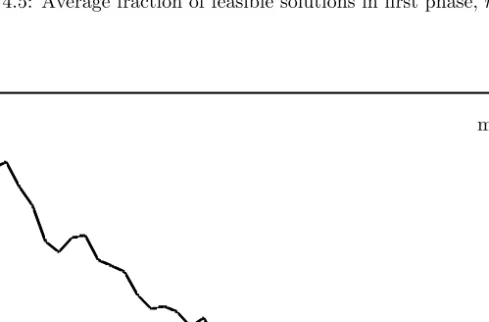
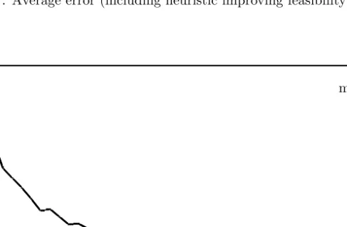
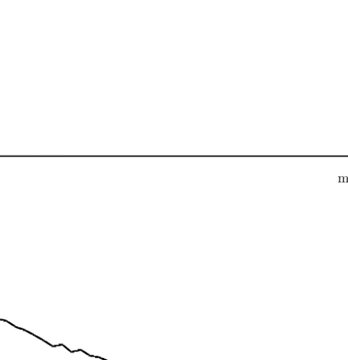
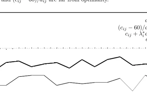
4.4.3 Computational results . . . 83
5 Asymptotically optimal greedy heuristics for the GAP 89 5.1 A family of pseudo-cost functions . . . 89
5.2 Geometrical interpretation . . . 91
5.3 Computational complexity of finding the best multiplier . . . 93
5.4 Probabilistic analysis . . . 94
5.4.1 A probabilistic model . . . 94
5.4.2 The optimal dual multipliers . . . 96
5.4.3 A unique vector of multipliers . . . 100
5.5 Numerical illustrations . . . 111
5.5.1 Introduction . . . 111
5.5.2 Comparison with Martello and Toth . . . 111
5.5.3 Improved heuristic . . . 113
III
Supply Chain Optimization in a dynamic environment121
6 Multi-Period Single-Sourcing Problems 123 6.1 Introduction . . . 1236.2 The model . . . 125
6.3 Reformulation as a CCAP . . . 129
6.3.1 Introduction . . . 129
6.3.2 The optimal inventory costs . . . 130
6.3.3 An equivalent CCAP formulation . . . 136
Contents 9
7 Feasibility analysis of the MPSSP 143
7.1 Introduction . . . 143
7.2 Stochastic model for the MPSSP . . . 145
7.3 Explicit feasibility conditions: the cyclic case . . . 146
7.4 Explicit feasibility conditions: the acyclic case . . . 147
7.4.1 Introduction . . . 147
7.4.2 Only dynamic assignments . . . 149
7.4.3 Identical facilities . . . 151
7.4.4 Seasonal demand pattern . . . 154
7.5 Numerical illustrations . . . 156
8 Asymptotical analysis of a greedy heuristic for the MPSSP 161 8.1 Introduction . . . 161
8.2 A family of pseudo-cost functions . . . 162
8.3 A probabilistic model . . . 163
8.4 An asymptotically optimal greedy heuristic: the cyclic case . . . 164
8.5 Asymptotic analysis: the acyclic case . . . 168
8.5.1 Introduction . . . 168
8.5.2 Only dynamic customers . . . 169
8.5.3 Static customers and seasonal demand pattern . . . 173
8.6 Numerical illustrations . . . 174
8.6.1 Introduction . . . 174
8.6.2 The cyclic case . . . 175
8.6.3 The acyclic case . . . 176
8.6.4 The acyclic and static case . . . 177
9 A Branch and Price algorithm for the MPSSP 183 9.1 Introduction . . . 183
9.2 The pricing problem for the static and seasonal MPSSP . . . 185
9.3 The pricing problem for the MPSSP . . . 188
9.3.1 General case . . . 188
9.3.2 The static case . . . 189
9.3.3 Dynamic case . . . 190
9.3.4 A class of greedy heuristics . . . 191
9.4 Numerical illustrations . . . 192
9.4.1 Introduction . . . 192
9.4.2 Description of the implementation . . . 193
9.4.3 Illustrations . . . 194
IV
Extensions
199
10 Additional constraints 201 10.1 Introduction . . . 20110.2 Throughput capacity constraints . . . 203
10.2.1 Introduction . . . 203
10.2.3 Generating experimental data . . . 205
10.2.4 A class of greedy heuristics . . . 206
10.2.5 A Branch and Price scheme . . . 208
10.3 Physical capacity constraints . . . 209
10.3.1 Introduction . . . 209
10.3.2 The optimal inventory holding costs . . . 209
10.3.3 Reformulation as a CCAP . . . 215
10.3.4 Generating experimental data . . . 216
10.3.5 A class of greedy heuristics . . . 217
10.3.6 A Branch and Price scheme . . . 218
10.4 Perishability constraints . . . 219
10.4.1 Introduction . . . 219
10.4.2 The optimal inventory holding costs . . . 219
10.4.3 Reformulation as a CCAP . . . 223
10.4.4 Generating experimental data . . . 224
10.4.5 A class of greedy heuristics . . . 224
10.4.6 A Branch and Price scheme . . . 226
11 A three-level logistics distribution network 229 11.1 Introduction . . . 229
11.2 The three-level MPSSP . . . 231
11.2.1 The model . . . 231
11.2.2 An equivalent assignment formulation . . . 233
11.2.3 The LP-relaxation . . . 238
11.2.4 Generating experimental data . . . 241
11.2.5 A class of greedy heuristics . . . 242
11.3 Throughput capacity constraints . . . 244
11.3.1 A reformulation . . . 244
11.3.2 Generating experimental data . . . 245
11.3.3 A class of greedy heuristics . . . 247
11.4 Physical capacity constraints . . . 249
11.4.1 A reformulation . . . 249
11.4.2 Generating experimental data . . . 252
11.4.3 A class of greedy heuristics . . . 252
11.5 Perishability constraints . . . 253
11.5.1 A reformulation . . . 253
11.5.2 Generating experimental data . . . 254
11.5.3 A class of greedy heuristics . . . 255
11.6 Numerical illustrations . . . 255
12 Summary and concluding remarks 259
Contents 11
Samenvatting (Summary in Dutch) 272
Part I
Optimization
in
Supply Chains
Chapter 1
Introduction
1.1
Distribution in a dynamic environment
Supply Chain Management is a field of growing interest for both companies and re-searchers. It consists of the management of material, information, and financial flows in a logistics distribution network composed of parties like vendors, manufacturers, distributors, and customers. The environment in which companies nowadays manage their supply chain is highly dynamic. This thesis is devoted to the development of optimization tools that enable companies to detect, and subsequently take advan-tage of, opportunities that may exist for improving the efficiency of their logistics distribution networks in such a dynamic environment.
Within the field of distribution logistics a number of developments have occurred over the past years. We have seen a globalization of supply chains in which na-tional boundaries are becoming less important. Within Europe we can observe an increase in the attention that is being paid by West-European companies to markets in Eastern Europe and the former Soviet Union. The fact that European borders are disappearing within the European Union results in questions about the realloca-tion, often concentrarealloca-tion, of production. Moreover, the relevance of European and regional distribution centers instead of national ones is reconsidered. According to Kotabe [80], the national boundaries are losing their significance as a psychological and physical barrier to international business. Therefore, companies are stimulated to expand their supply chains across different countries. Global supply chains try to take advantage of the differences in characteristics of various countries when de-signing their manufacturing and sourcing strategies. For example, the labor and raw materials costs are lower in developing countries while the latest advances in technology are present only in developed countries. As pointed out by Vidal and Goetschalckx [135], global supply chains are more complex than domestic ones be-cause, in an international setting, the flows in the supply chain are more difficult to coordinate. Issues that are exclusive to a global supply chain are different taxes, trade barriers, and transfer prices.
There are dynamics inherent to the flows in the supply chain. Fisher [46]
troduces the concepts functional and innovative to classify products. Functional products are the physical products without any added value in the form of, for in-stance, special packaging, fashionable design, service, etc. He argues that functional products have a relatively long life cycle, and thus a stable and steady demand, but often also low profit margins. Therefore, companies introduce innovations in fashion or technology with the objective of creating a competitive advantage over other suppliers of physically similar products, thereby increasing their margins. As a consequence, this leads to a shortening of the life cycle of innovative products since companies are forced to introduce new innovations to stay competitive. Another de-velopment that can be observed is the customer orientation. Supply chains have to satisfy the requirements of the customers with respect to the customized products as well as the corresponding services. The first step when designing and controlling an effective supply chain is to investigate the nature of the demand of the products. The tendency towards a shorter life cycle for innovative products leads to highly dynamic demand patterns and companies need to regularly reconsider the design of their supply chains to effectively utilize all the opportunities for profit.
One way of creating a competitive advantage is by maintaining a highly effective logistics distribution network. Thus, logistics becomes an integral part of the product that is being delivered to the customer. Competitiveness encourages a continuous improvement of the customer service level, see Ballou [6]. For example, one of the most influencing elements in the quality of the customer service is the lead time. Technological advances can be utilized to reduce these lead times, see Slats et al. [125]. For example, Electronic Data Interchange with or without internet leads to improved information flows, which yield a better knowledge of the customers’ needs at each stage of the supply chain.
Another way that a company can add value to its products to distinguish them from competing products is to take environmental issues into account, thereby cre-ating a so-called ‘green supply chain’, see Thomas and Griffin [130]. For further references on that topic see e.g. Bloemhof-Ruwaard et al. [18] and Fleischmann et al. [50].
The outline of this chapter is as follows. In Section 1.2 we describe the opportu-nities for increasing the efficiency of the supply chain that can be achieved by using Operations Research techniques. In Section 1.3 we will discuss the importance of co-ordination in the supply chain. In Section 1.4 we will state the necessity of a dynamic model when combining transportation and inventory decisions, or when dealing with products that show a strong seasonal component in their demand patterns or suffer from perishability. Finally, in Section 1.5 we will describe the goal of the thesis and we will briefly describe its contents. Some of the discussions in this chapter can be found in Romero Morales, Van Nunen and Romeijn [117].
1.2. Operations Research in Supply Chain Management 17
1.2
Operations Research in Supply Chain
Manage-ment
The mission of Operations Research is to support real-world decision-making using mathematical and computer modeling, see Luss and Rosenwein [86]. Supply Chain Management is one of the areas where Operations Research has proved to be a powerful tool, see Geunes and Chang [60] and Tayur, Ganeshan, and Magazine [129]. Bramel and Simchi-Levi [20] claim that, in logistics management practice, the tendency to use decision rules that were adequate in the past, or that seem to be intuitively good, is still often observed. However, it proved to be worthwhile us-ing scientific approaches to certificate a good performance of the supply chain or to detect opportunities for improving it. Many times this leads to a more effective performance of the supply chain while maintaining or even improving the customer service level. There are many examples of different scientific approaches used in the development of decision support systems (see e.g. Van Nunen and Benders [134], Benders et al. [13], and Hagdorn-van der Meijden [67]), or the development of new optimization models representing the situation at hand as closely as possible (see e.g. Geoffrion and Graves [58], Gelders, Pintelon and Van Wassenhove [56], Fleis-chmann [49], Chan, Muriel and Simchi-Levi [29], Klose and St¨ahly [77], and T¨ushaus and Wittmann [132]).
Geoffrion and Powers [59] summarize some of the main reasons for the increasing role of optimization techniques in the design of distribution systems. The most crucial one is the development of the capabilities of computers that allow for the investigation of richer and more realistic models than could be analyzed before. In these extended models, additional important issues, for e.g. scenario analysis, can be included. This development in computer technology is accompanied by new advances in algorithms, see Nemhauser [99].
The vast literature devoted to quantitative methods in Supply Chain Manage-ment also suggests the importance of Operations Research in this field. Bramel and Simchi-Levi [20] have shown the power of probabilistic analysis when defining heuristic procedures for distribution models. Geunes and Chang [60] give a survey of models in Operations Research emphasizing the design of the supply chain and the coordination of decisions. Tayur, Ganeshan and Magazine [129] have edited a book on quantitative models in Supply Chain Management. The last chapter of this book is devoted to a taxonomic review of the Supply Chain Management literature.
In a more practical setting, Gelders, Pintelon and Van Wassenhove [56] use a plant location model for the reorganization of the logistics distribution networks of two small breweries into a single bigger one. Shapiro, Singhal and Wagner [122] develop a Decision Support System based on Mathematical Programming tools to consolidate the value chains of two companies after the acquisition of the second by the first one. Arntzen et al. [4] present a multi-echelon multi-period model which was used in the reorganization of Digital Equipment Corporation. Hagdorn-van der Meijden [67] presents some examples of companies where new structures have been implemented recently. K¨oksalan and S¨ural [79] use a multi-period Mixed Integer Problem for the opening of two new malt plants for Efes Beverage. Myers [95]
presents an optimization model to forecast the demand that a company producing plastic closures can accommodate when these closures suffer from marketing perisha-bility. From an environmental point of view, decreasing the freight traffic is highly desirable. Kraus [81] claims that most of the environmental parameters for evalu-ating transportation in logistics distribution networks are proportional to the total distance traveled, thus a lot of effort is put into developing systems that decrease that distance.
1.3
Coordination in supply chains
A company delivers its products to its customers by using a logistics distribution network. Such a network typically consists of product flows from the producers to the customers through transshipment points, distribution centers (warehouses), and retailers. In addition, it involves a methodology for handling the products in each of the levels of the logistics distribution network, for example, the choice of an inventory policy, or the transportation modes to be used.
Designing and controlling a logistics distribution network involve different levels of decision-making, which are not independent of each other but exhibit interactions. At the operational level, day-to-day decisions like the assignment of the products ordered by individual customers to trucks, and the routing of those trucks must be taken. The options and corresponding costs that are experienced at that level clearly depend on choices that have been made at the longer term tactical level. The time horizon for these tactical decisions is usually around one year. Examples of decisions that have to be made at this level are the allocation of customers to warehouses and how the warehouses are supplied by the plants, the inventory policy to be used, the delivery frequencies to customers, and the composition of the transportation fleet. Clearly, issues that play a role at the operational level can dictate certain choices and prohibit others at the tactical level. For instance, the choice of a transportation mode may require detailed information about the current transportation costs which depend on decisions at the operational level. Similarly, the options and corresponding costs that are experienced at the tactical level clearly depend on the long-term strategic choices regarding the design of the logistics distribution network that have been made. The time horizon for these strategic decisions is often around three to five years. The most significant decisions to be made at this level are the number, the location and the size of the production facilities (plants) and distribution centers (warehouses). But again, issues that play a role at the tactical level could influence the options that are available at the strategic level. When designing the layout of the logistics distribution network we may need detailed information about the actual transportation costs, which is an operational issue as mentioned above.
To ensure an efficient performance of the supply chain, decisions having a signif-icant impact on each other must be coordinated. For instance, companies believe that capacity is expensive (see Bradley and Arntzen [19]). This has a twofold con-sequence. Firstly, the purchase of production equipment is made by top managers, while the production schedules and the inventory levels are decided at lower levels in the company. Therefore, the coordination between those decisions is often present
1.3. Coordination in supply chains 19
to a limit extent. Secondly, expensive equipment is often used to full capacity, which leads to larger inventories than necessary to meet the demand and causes an imbal-ance between capacity and inventory investments. Bradley and Arntzen [19] propose a model where the capacity and the inventory investments, and the production sched-ule are integrated and show the opportunities for improvement in the performance of the supply chain found in two companies.
Coordination is not only necessary between the levels of decision-making but also between the different stages of the supply chain, like procurement, production and distribution (see Thomas and Griffin [130]). In the past, these stages were managed independently, buffered by large inventories. The decisions in different stages were often decoupled since taking decisions in just one of these stages was already a com-prehensive task in itself. For example, from a computational point of view, just the daily delivery of the demand of a set of customers is a hard problem. Decoupling decisions in different stages causes larger costs and longer delivery times. Nowadays, the fierce competition in the market forces companies to be more efficient by taking decisions in an integrated manner. This has been possible due to the tremendous de-velopment of computer capabilities and the new advances in algorithms, see Geoffrion and Powers [59].
Several examples can be found in the literature proving that models coordinating at least two stages of the supply chain can detect new opportunities that may exist for improving the efficiency of the supply chain. For instance, Chandra and Fisher [30] propose two solution approaches to investigate the impact of coordination of pro-duction and distribution planning. They consider a single-plant, multi-product, and multi-period scenario. The plant produces and stores products for a while. After that, they are delivered to the retailers (customers) by a fleet of trucks. One of the solution approaches tackles the production scheduling and the routing problems sep-arately. They compare this approach to a coordinated approach where both decisions are incorporated in one model. In their computational study, they show that the co-ordinated approach can yield up to 20% in costs savings. Anily and Federgruen [3] study a model integrating inventory control and transportation planning decisions motivated by the trade-off between the size and the frequency of delivery. They consider a single-warehouse and multi-retailer scenario where inventory can only be kept at the retailers which face constant demand. The model determines the replen-ishment policy at the warehouse and the distribution schedule for each retailer so that the total inventory and distribution costs are minimized. They present heuristic procedures to find upper and lower bounds on the optimal solution value.
Models coordinating different stages of the supply chain can be again classified as strategic, tactical or operational. Several surveys can be found in the litera-ture addressing coordination issues. Beamon [11] summarizes models in the area of multi-stage supply chain design and analysis. Ereng¨u¸c, Simpson and Vakharia [39] survey models integrating production and distribution planning. Thomas and Grif-fin [130] survey coordination models on strategic and operational planning. Vidal and Goetschalckx [135] pay attention to strategic production-distribution models with special emphasis on global supply chain models. Bhatnagar, Chandra and Goyal [15] call the coordination between the three stages of the supply chain ‘general
coordination’. They also describe the concept of multi-plant coordination, i.e., the coordination of production planning among multiple plants, and survey the literature on this topic.
1.4
A dynamic model for evaluating logistics
net-work designs
When opportunities for improvement in the design of a logistics distribution network are present, management can define alternatives to the current design. In order to be able to evaluate and compare these alternatives, various performance criteria (under various operating strategies) need to be defined. An example of such a criterion could be total operational costs, see Beamon [11].
There are many examples of products where the production and distribution environment is dynamic, for instance because the demand contains a strong seasonal component. For example, the demand for soft drinks and beers is heavily influenced by the weather, leading to a much higher demand in warmer periods. A rough representation of the demand pattern, disregarding the stochastic component due to daily unpredictable/unforeseeable changes in the weather, will show a peak in summer and a valley in winter. Nevertheless, most of the existing models in the literature are static (single-period) in nature. This means that the implicit assumption is made that the environment, including all problem data, are constant over time. For instance, demand patterns are assumed to be constant, even though this is often an unrealistic assumption. Hence, the adequacy of those models is limited to situations where the demand pattern exhibits no remarkable changes throughout the planning horizon. In practice, it means that all, by nature dynamic, input parameters to the model are approximated by static ones like average parameters.
The simplest approach to deal with this issue could be a two-phase procedure where we first solve a suitable static model and in the second phase try to obtain a solution to the actual problem. For example, Van Nunen and Benders [134] use only the data corresponding to the peak season for their medium and long-term analysis. At the other end of the spectrum, an approach could be to define the parameters of the model and the decisions to be taken as functions of time, and impose that capacity constraints must be satisfied at each point in time. The difficulties present in the data estimation, the analysis of the model, as well as the implementation of the solution (if one can be found) make this approach rather impractical. As mentioned above, the literature focuses mainly on static models. There are notable exceptions where the planning horizon is discretized. Duran [37] plans the production, bottling, and distribution to agencies of different types of beer, with an emphasis on the production process. A one year planning horizon is considered, but in contrast to most of the literature, the model is dynamic with twelve monthly periods. Chan, Muriel and Simchi-Levi [29] study a dynamic, but uncapacitated, distribution problem in an operational setting. Arntzen et al. [4] present a multi-echelon multi-period model with no single-sourcing constraints on the assignment variables which was used in the reorganization of Digital Equipment Corporation.
1.5. Goal and summary of the thesis 21
Following those models, we will also discretize the planning horizon, thereby closely approximating the true time-dependent behaviour of the data. We propose splitting the planning horizon into smaller periods where demands in each period are forecasted by constant values. (Note that it is not required that the periods are of equal length!) This means that, implicitly, we are assuming that the demand has a stationary behaviorin each period.
Another advantage of a dynamic approach to the problem is the ability to ex-plicitly model inventory decisions. This enables us to jointly estimate transportation and inventory costs. Recall that this is not possible when considering an aggregate single-period representation of the problem. Our model can also deal with products having a limited shelf-life, in other words, products that suffer from perishability. This can be caused by the fact that the product exhibits a physical perishability or it might be affected by an economic perishability (obsolescence). In both cases, the storage duration of the product should be limited. Perishability constraints have mainly been taken into account in inventory control, but they can hardly be found in the literature on Physical Distribution. A notable exception is Myers [95], who presents a model where the maximal demand that can be satisfied for a given set of capacities and under perishability constraints is calculated.
1.5
Goal and summary of the thesis
The goal of this thesis is the study of optimization models, which integrate both transportation and inventory decisions, to search for opportunities for improving the logistics distribution network. In contrast to Anily and Federgruen [3], who also study a model integrating these two aspects in a tactical-operational setting, we utilize the models to answer strategic and tactical questions. We evaluate an estimate of the total costs of a given design of the logistics distribution network, including production, handling, inventory holding, and transportation costs. The models are also suitable for clustering customers with respect to the warehouses, and through this they can be used as a first step towards estimating operational costs in the logistics distribution network related to the daily delivery of the customers in tours.
The main focus of this thesis is the search for solution procedures for these opti-mization models. Their computational complexity makes the use of heuristics solu-tion procedures for large-size problem instances advisable. We will look for feasible solutions with a class of greedy heuristics. For small or medium-size problem in-stances, we will make use of a Branch and Price scheme. Relevant characteristics of the performance of a solution procedure are the computation time required and the quality of the solution obtained if an optimal solution is not guaranteed. Conclu-sions about these characteristics are drawn by testing it on a collection of problem instances. The validity of the derived conclusions strongly depends on the set of problem instances chosen for this purpose. Therefore, the second focus of this thesis is the generation of experimental data for these optimization models to test these solution methods adequately.
model to evaluate a two-level logistics distribution network where production and storage take place at the same location. Moreover, some of the dynamic models analyzed in this thesis can be reformulated as a GAP with a nonlinear objective function. Therefore, we will devote Part II of the thesis to studying this problem. In Parts III and IV we will study variants of a multi-period single-sourcing problem (MPSSP) that can be used for evaluating logistics distribution network designs with respect to costs in a dynamic environment. In particular, Part III is dedicated to the analysis of a logistics distribution network where production and storage take place at the same location and only the production capacity is constrained. In Chapter 10, we will separately add different types of capacity constraints to this model. In par-ticular, we will analyze the addition of constraints with respect to the throughput of products and the volume of inventory. Furthermore, we will analyze how to deal with perishable products. In Chapter 11, we will study models in which the production and storage levels are separated.
In Parts III and IV, the customers’ demand patterns for a single product are assumed to be known and each customer needs to be delivered by a unique warehouse in each period. The decisions that need to be made are (i) the production sites and quantities, (ii) the assignment of customers to facilities, and (iii) the location and size of inventories. These decisions can be handled in a nested fashion, where we essentially decide on the assignment of customers to facilities only, and where the production sites and quantities, and the location and size of inventories are determined optimally as a function of the customer assignments. Viewed in this way, the MPSSP is a generalization of the GAP with a convex objective function, multiple resource requirements, and possibly additional constraints, representing, for example, throughput or physical inventory capacities, or perishability of the product.
To be able to deal with many variants of the MPSSP using a single solution approach, we will introduce in Chapter 2 a general class of convex capacitated as-signment problems (CCAP’s). A distinguished member of this class is the GAP. As mentioned above, we are concerned with adequately testing solution procedures for the CCAP. Therefore, we will introduce a general stochastic model for the CCAP, and derive tight conditions to ensure asymptotic feasibility in a probabilistic sense. To solve the CCAP, we have proposed two different solution methods. Firstly, we have generalized the class of greedy heuristics proposed by Martello and Toth [88] for the GAP to the CCAP and we have proposed two local exchange procedures for improving a given (partial) solution for the CCAP. Secondly, we have generalized the Branch and Price scheme given by Savelsbergh [121] for the GAP to the CCAP and have studied the pricing problem for a particular subclass of CCAP’s for which bounds can be efficiently found.
Throughout Parts II-IV our goal will be to analyze the behaviour of the solution methods proposed in Chapter 2. We will show asymptotic feasibility and optimality of some members of the class of greedy heuristics for the CCAP for the particular case of the GAP. Similar results will be found for many variants of the MPSSP. We will show that the Branch and Price scheme is another powerful tool when solving MPSSP’s to optimality. Our main concern will be to identify subclasses of these optimization models for which the pricing problem can be solved efficiently.
1.5. Goal and summary of the thesis 23
The outline of the thesis is as follows. In Chapter 2 we introduce the class of CCAP’s and present a general stochastic model for the CCAP and tight conditions to ensure asymptotic feasibility in a probabilistic sense. Moreover, we introduce a class of greedy heuristics and two local exchange procedures for improving a given (partial) solution for the CCAP, and a Branch and Price scheme together with the study of the pricing problem for a subclass of CCAP’s. Part II is devoted to the study of the GAP which, as mentioned above, is a static model to evaluate two-level logistics distribution networks where production and storage take place at the same location. In Chapter 3 we show that the GAP belongs to the class of CCAP’s, summarize the literature devoted to this problem, and we present some properties of the GAP which will be used in the rest of Part II. In Chapter 4 we analyze almost all the random generators proposed in the literature for the GAP and we numerically illustrate how the conclusions drawn about the performance of a greedy heuristic for the GAP differ depending on the random generator used. In Chapter 5 we show that, for large problem instances of the GAP generated by a general stochastic model, two greedy heuristics, defined by using some information of the LP-relaxation of the GAP, find a feasible and optimal solution with probability one. Part III is devoted to the study of a class of two-level MPSSP’s where production and storage take place at the same location and only the production capacity is constrained. In Chapter 6 we introduce this class, we show that it is contained in the class of CCAP’s, and we present some properties which will be used in the rest of this part. In Chapter 7, as for the GAP, we find explicit conditions to ensure asymptotic feasibility in the probabilistic sense for some variants of the MPSSP. In Chapter 8 we show that, for large problem instances of the MPSSP generated by a general stochastic model, a greedy heuristic, defined by using some information of the LP-relaxation of the MPSSP, finds a feasible and optimal solution with probability one for some variants of the MPSSP, as for the GAP. In Chapter 9 we analyze the pricing problem for the MPSSP and we propose a class of greedy heuristics to find feasible solutions for the pricing problem. In Part IV we extend the model proposed in Part III in two directions. In Chapter 10 we show that the MPSSP with three different types of additional constraints, namely throughput capacity, physical capacity and perishability constraints, can still be reformulated as a CCAP and we apply the results derived for the CCAP. In Chapter 11 we study three-level logistics distribution networks in which the plants and the warehouses have been decoupled, we show that these models can be almost reformulated as CCAP’s, and that, except for the Branch and Price scheme, all the results derived for the CCAP still hold for these models. We end the thesis in Chapter 12 with a summary and some concluding remarks.
Chapter 2
A Class of Convex
Capacitated Assignment
Problems
2.1
Introduction
In a general assignment problem there are tasks which need to be processed and agents which can process these tasks. Each agent faces a set of capacity constraints and a cost when processing the tasks. Then the problem is how to assign each task to exactly one agent, so that the total cost of processing the tasks is minimized and each agent does not violate his capacity constraints. In the class of Convex Capacitated Assignment Problems (CCAP) each capacity constraint is linear with nonnegative coefficients and the costs are given by a convex function. The problem can be formulated as follows:
minimize m X i=1 gi(xi·) subject to Aixi· ≤ bi i= 1, . . . , m m X i=1 xij = 1 j= 1, . . . , n xij ∈ {0,1} i= 1, . . . , m;j= 1, . . . , n
where gi : Rn → R is a convex function, Ai ∈ Mki×n is a nonnegative matrix,
and bi ∈ Rki is a nonnegative vector. Hereafter we will represent matrix Ai by
its columns, i.e., Ai = (Ai1|. . .|Ain) where Aij ∈ R
ki for each j = 1, . . . , n. The
constraints associated with agent i,Aix
i·≤bi, define the feasible region of a
multi-knapsack problem.
Other classes of assignment problems have been proposed in the literature. Fer-land, Hertz and Lavoie [43] introduce a more general class of assignment problems, and show the applicability of object-oriented programming by developing software containing several heuristics. All set partitioning models discussed by Barnhart et al. [9] with convex and separable objective function in the index i are examples of convex capacitated assignment problems. They focus on branching rules and some computational issues relevant in the implementation of a Branch and Price scheme. In a similar context, Freling et al. [52] study the pricing problem of a class of convex assignment problems where the capacity constraints associated with each agent are defined by general convex sets.
TheGeneralized Assignment Problem (GAP) is one of the classical examples of a convex capacitated assignment problem (Ross and Soland [118]), where the cost function gi associated with agent i is linear inxi· and just one capacity constraint
is faced by each agent, i.e., ki = 1 for each i = 1, . . . , m. The GAP models the
situation where a single resource available at the agents is consumed when processing tasks. Gavish and Pirkul [55] have studied a more general model, the Multi-Resource Generalized Assignment Problem (MRGAP) where several resources are available at the agents. This is still an example of a convex capacitated assignment problem where the objective function is linear as for the GAP, and each agent faces the same number of capacity constraints, i.e., ki =k for each i = 1, . . . , m. Ferland, Hertz
and Lavoie [44] consider an exchange procedure for timetabling problems where the capacity constraints are not necessarily separable in the agents and the objective function is linear. Mazzola and Neebe [92] propose a Branch and Bound procedure for the particular situation where each agent must process exactly one task. This model can be seen as the classical Assignment Problem (see Nemhauser and Wolsey [100]) with side constraints.
Since the GAP is anN P-Hard problem (see Martello and Toth [89]), so is the CCAP. Moreover, since the decision problem associated with the feasibility of the GAP is anN P-Complete problem, so is the corresponding decision problem for the CCAP. Therefore, even to test whether a problem instance of the CCAP has at least one feasible solution is computationally hard. Hence, solving large problem instances to optimality may require a significant computational effort. The quality of the solution required and the technical limitations will determine the type of solution procedure to be used.
The outline of this chapter is as follows. In Section 2.2 we will introduce a general stochastic model for the class of convex capacitated assignment problems, and derive tight conditions to ensure asymptotic feasibility in a probabilistic sense when the number of tasks grows to infinity. In Section 2.3 we propose a class of greedy heuristics for the CCAP as well as two local exchange procedures for improving a given (partial) solution for the CCAP. In Section 2.4 each convex capacitated assignment problem is equivalently formulated as a set partitioning problem. In Section 2.5 we propose a Branch and Price procedure for solving this problem based on a column generation approach for the corresponding set partitioning formulation. This approach generalizes a similar Branch and Price procedure for the GAP (see Savelsbergh [121]). In Section 2.5.4 we study the pricing problem for a particular
2.2. Stochastic models and feasibility analysis 27
subclass for which efficient bounds can be found. The chapter ends in Section 2.6 with a summary. Some of the results in this chapter can be found in Freling et al. [52].
2.2
Stochastic models and feasibility analysis
2.2.1
A general stochastic model
Solution procedures are meant to give answers to real-life problem instances. Gen-erally, real data is only available for few scenarios. The limitation on the number of the data sets can bias the conclusions drawn about the behavior of the solution procedures. Thus, problem instances are generated to validate solution procedures. However, data generation schemes may also introduce biases into the computational results, as Hall and Posner [68] mention. They consider the feasibility of the problem instances an important characteristic of a data generation scheme. They propose two approaches to avoiding infeasible problem instances. The first one is to generate problem instances without regard for feasibility and discard the infeasible ones, and the second one is to enforce feasibility in the data generation process. Obviously, the first approach can be very time consuming when the generator of problem instances is not adequate.
Probabilistic analysis is a powerful tool when generating appropriate random data for a problem. Performing a feasibility analysis yields a suitable probabilistic model that can be used for randomly generating experimental data for the problem, with the property that the problem instances are asymptotically feasible with probability one. In this respect, Romeijn and Piersma [110] propose a stochastic model for the GAP where for each task the costs and requirements are i.i.d. random vectors, and the capacities depend linearly on the number of tasks. By means of empirical process theory, they derive a tight condition to ensure feasibility with probability one when the number of tasks goes to infinity. They also perform a value analysis of the GAP. In the literature we mainly find probabilistic value analyses. They have been performed for a large variety of problems, starting with the pioneering paper by Beardwood, Halton and Hammersley [12] on a probabilistic analysis of Euclidean TSP’s, spawning a vast number of papers on the probabilistic analysis of various variants of the TSP and VRP (see Bramel and Simchi-Levi [20] for an overview, and, for a more recent example, the probabilistic analysis of the inventory-routing problem by Chan, Federgruen and Simchi-Levi [28]).
Numerous other problems have also been analyzed probabilistically. Some well-known examples are a median location problem (Rhee and Talagrand [107]), the multi-knapsack problem (Van de Geer and Stougie [133]), a minimum flow time scheduling problem (Marchetti Spaccamela et al. [87]), the parallel machine schedul-ing problem (Piersma and Romeijn [104]), a generalized bin-packschedul-ing problem (Feder-gruen and Van Ryzin [41]), the flow shop weighted completion time problem (Kamin-sky and Simchi-Levi [73]), and the capacitated facility location problem (Piersma [103]). All these applications have in common that feasibility is not an issue since feasible problem instances can easily be characterized, so that a probabilistic analysis
of the optimal value of the optimization problem suffices.
As mentioned above, we will perform a feasibility analysis of the CCAP. Thus, when defining a stochastic model for the CCAP we can leave out parameters defin-ing the objective function. Note that this does not preclude correlations between parameters. Consider the following probabilistic model for the parameters defining the feasible region of the CCAP. Let the random vectorsAj = ((A1j)>, . . . ,(A
m j )>)>
(j = 1, . . . , n) be i.i.d. in the bounded set [A, A]k1 ×. . .×[A, A]km where A and
A∈R+. Furthermore, letbi depend linearly onn, i.e.,bi =βin, for positive vectors
βi ∈Rki. Observe thatm and k
i are fixed, thus the size of each problem instance
only depends on the number of tasksn. Even though the requirements must be iden-tically distributed, by considering the appropriate mixture of distribution functions, this stochastic model is suitable to model several types of tasks.
To analyze probabilistically the feasibility of the CCAP, we will use the same methodology as Romeijn and Piersma [110] for the GAP. They consider an auxiliary mixed integer linear problem to decide whether a given problem instance of the GAP has at least a feasible solution, or additional capacity is needed to ensure feasibility. A relationship between the optimal solution values of the auxiliary problem and its LP-relaxation is established. Through empirical process theory, the behaviour of the LP-relaxation is characterized. Altogether this yields a tight condition that ensures asymptotic feasibility with probability one when the number of tasks grows to infinity. In the next section we will summarize the results used from empirical process theory.
2.2.2
Empirical processes
LetS be a class of subsets of some space X. Forndistinct pointsx1, . . . , xn inX,
define
∆S(x1, . . . , xn)≡card(S∩ {x1, . . . , xn}:S∈ S),
so, ∆S(x1, . . . , xn) counts the number of distinct subsets of{x1, . . . , xn}that can be
obtained when {x1, . . . , xn} is intersected with sets in the classS. Also define
mS(n)≡sup{∆S(x1, . . . , xn) :x1, . . . , xn∈X}.
The class S is called a Vapnik-Chervonenkis class (orVC class) if mS(n)<2n for
some n≥1.
For any subsetY ofRm, define the graph of a functionf :Y →Rby
graph(f)≡ {(s, t)∈ Y ×R: 0≤t≤f(s) orf(s)≤t≤0}.
A class of real-valued functions is called aVapnik-Chervonenkis graph class (orVC graph class) if the class of graphs of the functions is a VC class.
Theorem 2.2.1 (cf. Talagrand [128]) LetX1,X2,. . .be a sequence of i.i.d. random variables taking values in a space(X,A)and letGbe a class of measurable real-values
functions on X, such that
2.2. Stochastic models and feasibility analysis 29
• the functions inG are uniformly bounded.
Then there exist` andR such that, for alln≥1 andδ >0, Pr sup g∈G 1 n n X j=1 g(xj)− Eg(x1) > δ ≤ Kδ√n `R ` ·exp −2δ 2n R
whereK is a universal constant not depending on(X,A)orG.
A more extensive introduction to empirical processes can be found in Piersma [102] where probabilistic analyses are performed on several classical combinatorial problems.
2.2.3
Probabilistic feasibility analysis
The auxiliary problem (F) to characterize the feasibility of a convex capacitated assignment problem can be defined as
maximize ξ subject to (F) Aixi· ≤ bi−ξeki i= 1, . . . , m m X i=1 xij = 1 j= 1, . . . , n xij ∈ {0,1} i= 1, . . . , m; j= 1, . . . , n ξ free whereeki denotes the vector in
Rki with all components equal to one. Note that this
problem always has a feasible solution. Letvn be the optimal value of (F), and vnLP
be the optimal value of the LP-relaxation of (F). The convex capacitated assignment problem is feasible if and only ifvn≥0.
When empirical process theory is used to perform the probabilistic analysis, an essential task is to establish a relationship between the optimal solution values of the problem and its LP-relaxation. The following lemma shows that the values vn and
vnLP remain close, even ifngrows large.
Lemma 2.2.2 The difference between the optimal solution values of (F) and its LP-relaxation satisfies: vLPn −vn≤ m X i=1 ki ! ·A.
Proof: Rewrite the problem (F) with equality constraints and nonnegative variables only. We then obtain a problem with, in addition to the assignment constraints,
Pm
of (F). The number of variables having a nonzero value in this solution is no larger than the number of equality constraints in the reformulated problem. Since there is at least one nonzero assignment variable corresponding to each assignment constraint, and exactly one nonzero assignment variable corresponding to each assignment that is feasible with respect to the integrality constraints of (F), there can be no more than Pm
i=1ki assignments that are split. Converting the optimal LP-solution to a
feasible solution to (F) by arbitrarily changing only those split assignments yields a solution to (F) that exceeds the LP-solution value by at most (Pm
i=1ki)·A. Thus
the desired inequality follows. 2
The following theorem uses empirical process theory to characterize the behaviour of the random variablevLP
n .
In the following,λ= (λ>1, . . . , λ>m)> whereλi∈Rki.
Theorem 2.2.3 There exist constants `F and R1 such that, for each n ≥ 1 and
δ >0, Pr 1nvLPn −∆ > δ ≤ Kδ√n `FR1 `F ·exp −2δ 2n R2 1
whereK is a universal constant, ∆ = min λ∈S m X i=1 λ>i βi− E min i=1,...,mλ > i A i 1 !
andS is the unit simplex inRk1×. . .× Rkm.
Proof: Dualizing the capacity constraints in (F) with parametersλi∈Rk+i, for each
i= 1, . . . , m, yields the problem maximizeξ+ m X i=1 λ>i bi−ξeki−Aixi· subject to m X i=1 xij = 1 j= 1, . . . , n xij ∈ {0,1} i= 1, . . . , m;j = 1, . . . , n ξ free.
Rearranging the terms in the objective function, we obtain
1− m X i=1 λ>i eki ! ·ξ+ m X i=1 λ>i bi− m X i=1 λ>i Aixi·= = 1− m X i=1 ki X k=1 λik ! ·ξ+ m X i=1 λ>i bi− m X i=1 n X j=1 λ>i A i jxij.
2.2. Stochastic models and feasibility analysis 31
Now let vn(λ) denote the optimal value of the relaxed problem. By strong duality,
vnLP = minλ≥0vn(λ). First observe that if P m i=1
Pki
k=1λik 6= 1, then vn(λ) = ∞.
Thus, we can restrict the feasible region of the relaxed problem to the simplex S. But in this case the optimal solution of the relaxed problem is attained for
• ξ= 0; and
• xij = 1 if i = arg minν=1,...,mλ>νAνj (where ties are broken arbitrarily), and
xij = 0 otherwise.
Then we have that
vn(λ) = m X i=1 λ>i bi− n X j=1 min i=1,...,mλ > i A i j = n X j=1 m X i=1 λ>i βi− min i=1,...,mλ > i A i j ! .
Now define the function fλ: [A, A]k1×. . .×[A, A]km →Rby
fλ(u) = m X i=1 λ>i βi− min i=1,...,mλ > i ui so that vn(λ) = n X j=1 fλ(Aj)
whereAj is a realization of the random vectorAj. The function classF={fλ:λ∈
S} is a VC graph class, since we can write graph(fλ) = = m [ i=1 ( (u, w)∈Rk1×. . .×Rkm×R: 0≤w≤ m X ν=1 λ>νβν−λ>i ui ) [ m \ i=1 ( (u, w)∈Rk1×. . .× Rkm×R: 0≥w≥ m X ν=1 λ>νβν−λ>i ui ) .
Moreover, this class is uniformly bounded, since
−A≤fλ(u)≤ m X i=1 ki X k=1 βik
for eachu∈[A, A]k1×. . .×[A, A]km. Noting that
n1vLPn −∆ = 1 nmin λ∈S n X j=1 fλ(Aj)−min λ∈SEfλ(A1) ≤ sup λ∈S 1 n n X j=1 fλ(Aj)− Efλ(A1) ,
the result now follows directly from Theorem 2.2.1. 2 The bound on the tail probability given in the last theorem will be used to show a tight condition to ensure feasibility with probability one whenngrows to infinity. This is a generalization of Theorem 3.2 from Romeijn and Piersma [110].
Theorem 2.2.4 As n → ∞, the CCAP is feasible with probability one if ∆ > 0, and infeasible with probability one if∆<0.
Proof: Recall that the CCAP is feasible if and only ifvn is nonnegative. Therefore,
Pr(the CCAP is feasible) = Pr(vn ≥0)
≤ Pr(vLPn ≥0) = Pr(1 nv LP n −∆≥ −∆) ≤ Pr(|1 nv LP n −∆| ≥ −∆).
It follows that the CCAP is feasible with probability zero (and thus infeasible with probability one) if ∆<0 since then, for 0< ε <−∆,
Pr |1 nv LP n −∆| ≥ −∆ ≤ Pr(|1 nv LP n −∆|> ε) ≤ Kε√n `FR1 `F ·exp −2ε 2n R2 1 by Theorem 2.2.4, and ∞ X n=1 Kε√n `FR1 `F ·exp −2ε 2n R2 1 <∞.
Similarly, by using Lemma 2.2.2
Pr(the CCAP is infeasible) = Pr(vn<0)
≤ Pr vLPn − m X i=1 ki ! ·A <0 ! = Pr 1 nv LP n −∆< m X i=1 ki ! ·A/n−∆ ! ≤ Pr |1 nv LP n −∆|>∆− m X i=1 ki ! ·A/n ! .
It follows that the CCAP is infeasible with probability zero (and thus feasible with probability one) if ∆>0 since then, forn >(Pm
i=1ki)·A/∆, Pr |1 nv LP n −∆|>∆− m X i=1 ki ! ·A/n ! ≤ ≤ K(∆n−(Pm i=1ki)·A) `FR1 √ n `F ·exp −2(∆n−( Pm i=1ki)·A) 2 nR2 1
2.2. Stochastic models and feasibility analysis 33 by Theorem 2.2.4, and X n>(Pm i=1ki)·A/∆ K(∆n−(Pm i=1ki)·A) `FR1 √ n `F · exp −2(∆n−( Pm i=1ki)·A)2 nR2 1 <∞. 2
For the case of the GAP, this result reduces to the one derived by Romeijn and Piersma [110]. This is an implicit condition which, most of the times, is difficult to check. They were only able to find explicit conditions when the requirements were agent-independent, i.e. Ai
j = Dj for each i = 1, . . . , m. In this case, the problem
defining the value of ∆ turns into a linear one. (Recall that for the GAP Aij are scalars.) So, the minimization can be reduced to inspecting the extreme points of the unit simplex inRm. For a general convex capacitated assignment problem, the
presence of the multi-knapsack constraints for each agent make it impossible to use the same reasoning.
In Chapter 7 we will encounter special cases of the CCAP for which the feasibility condition that ∆>0 can also be made explicit. However, for some of the variants of these CCAP’s, this stochastic model is not suitable since it imposes independence be-tween the requirement vectors. In the following section, we will extend the stochastic model for the CCAP given in Section 2.2.1 to be able to deal also with these cases.
2.2.4
Extension of the stochastic model
The stochastic model for the CCAP given in Section 2.2.1 assumes that the vector of requirements of the tasks Aj (j = 1, . . . , n) are independently distributed. In
Chapter 7 we will see that this condition is not fulfilled in some examples of CCAP’s. In this section, we relax the independence assumption in the following way. We will generate the requirement parameters for subsets of tasks, so that the vectors of requirement parameters corresponding to different subsets are independently and identically distributed. Note that we do not impose any condition on the requirements of the tasks within the same subset. More precisely, letJjbe thej-th subset of tasks
and, for now, assume that|Jj|=J for eachj = 1, . . . , n. Observe that the number
of tasks in the CCAP formulation is now equal to nJ. For each j = 1, . . . , n and
`= 1, . . . , J, letAJj`denote the vector of requirements of the`-th task in the subset
Jj. Let the random vectorsAJj = (A
>
Jj`)
>
`∈Jj (j= 1, . . . , n) be i.i.d. in the bounded
set QJ
`=1 [A, A]
k1×. . .×[A, A]kmwhere AandA∈
R+. As before, letbi depend
linearly on n, i.e.,bi=βin, for positive vectorsβi∈Rki.
In the following theorem we show a similar condition as in Theorem 2.2.4 to ensure feasibility with probability one when n grows to infinity. In this case the
excess capacity reads as follows: ∆ = min λ∈S m X i=1 λ>i βi− J X `=1 E min i=1,...,mλ > i A i J1` !
whereS is the unit simplex in Rk1×. . .× Rkm.
Theorem 2.2.5 As n → ∞, the CCAP is feasible with probability one if ∆ > 0, and infeasible with probability one if∆<0.
Proof: From the proof of Theorem 2.2.4, it is enough to show that there exist constants` andRsuch that, for eachn≥1 andδ >0, we have that
Pr 1nvLPn −∆ > δ ≤ Kδ√n `R ` ·exp −2δ 2n R2 .
Following similar steps as in the proof of Theorem 2.2.3, we have that vLP
n = minλ≥0vn(λ) where vn(λ) = n X j=1 m X i=1 λ>i βi− J X `=1 min i=1,...,mλ > i A i Jj` ! .
Now define the function fλ:QJ`=1 [A, A]k1×. . .×[A, A]km→Rby
fλ(u) = m X i=1 λ>i βi− J X `=1 min i=1,...,mλ > i ui` so that vn(λ) = n X j=1 fλ(AJj)
whereAJj is a realization of the random vectorAJj. With the same arguments as in
Theorem 2.2.3, we can show that the function classF={fλ:λ∈S}is a VC graph
class and uniformly bounded, and the result follows similarly to Theorem 2.2.3. 2 A similar result can be obtained when the size of the subsets generated is not unique but it can takeκvalues, sayJs, for eachs= 1, . . . , κ. We will assume that the
size of the subsets of tasks is multinomial-distributed with parameters (π1, . . . , πκ),
with πs≥0 and Pκs=1πs= 1, whereπs is the probability of generating a subset of
Jstasks. Observe that the number of tasks in the CCAP formulation is random and
equal to Pn
j=1Jj. For eachj = 1, . . . , n, s = 1, . . . , κ, and `= 1, . . . , J, let AJjs`
denote the vector of requirements of the`-th task in the subsetJjwhen|Jj|=Js. Let
the random vectorsAJj = ((A
> Jj1`) > `∈Jj, . . . ,(A > Jjκ`) > `∈Jj) > (j= 1, . . . , n) be i.i.d. in
the bounded setQκ
s=1
QJs
`=1 [A, A]
k1×. . .×[A, A]km whereA andA∈
R+. Note that only one of the vector of requirements, say (A>J
js`)
>
2.2. Stochastic models and feasibility analysis 35
subsetJj, depending on the realized number of tasks in that subset. As before, let
bi depend linearly onn, i.e.,bi=βin, for positive vectorsβi∈Rki.
In this case, the excess capacity reads ∆ = min λ∈S m X i=1 λ>i βi− κ X s=1 πs Js X `=1 E min i=1,...,mλ > i A i J1s` !
whereSis the unit simplex inRk1×. . .×
Rkm. Then, the tight condition for feasibility
reads as follows.
Theorem 2.2.6 As n → ∞, the CCAP is feasible with probability one if ∆ > 0, and infeasible with probability one if∆<0.
Proof: Similar to the proof of Theorem 2.2.5. 2
2.2.5
Asymptotically equivalent stochastic models
The stochastic model for the CCAP introduced above considers deterministic right-hand sides. This excludes, for example, cases where right-right-hand sides depend on the requirements of the tasks which is widely used in random generators for the GAP, as will be shown in Chapter 4. Stochastic models with random right-hand sides where the relative capacities in the infinity are constant can be still analyzed by means of the concept of asymptotically equivalent stochastic models. It can be shown that feasibility conditions are the same for asymptotically equivalent stochastic models. Therefore, we can obtain a similar result to Theorem 2.2.4. Hereafter (A,b) will denote a stochastic model for the parameters of the feasible region of the CCAP where A= (Aj), Aj represents the vector of requirements for taskj, b= (bi) and
bi is the right-hand side vector associated with agenti.
Definition 2.2.7 Let(A,b)and(A0,b0)be two stochastic models for the feasible re-gion of the CCAP. We will say that(A,b)and(A0,b0)are asymptotically equivalent if the following statements hold:
1. Requirements are equally distributed in both of the models. 2. For eachi= 1, . . . , mandk= 1, . . . , ki, it holds
bik−b0ik
n → 0
with probability one whenn goes to infinity.
In the next result we show that feasibility conditions are the same for asymptot-ically equivalent stochastic models.
Proposition 2.2.8 Let(A,b)and(A0,b0)be two asymptotically equivalent stochas-tic models for the parameters defining the feasible region of the CCAP. Then, (A,b) is feasible with probability when n goes to infinity if and only if (A0,b0) is feasible with probability one whenngoes to infinity.
Proof: Let vLPn be the random variable defined as the optimal value of the LP-relaxation of (F) for the stochastic model (A,b) andv0n
LP for (A0,b0). It is enough to prove that 1 n|vn LP−v0 n LP | →0
with probability one whenn goes to infinity. From the proof of Theorem 2.2.3, we know that vLPn = min λ∈S m X i=1 λ>i bi− n X j=1 min i=1,...,mλ > i A i j ,
and similarly forv0nLP. So, 1 n|v LP n −v 0 n LP |= = 1 n min λ∈S m X i=1 λ>i bi− n X j=1 min i=1,...,mλ > i A i j −min λ∈S m X i=1 λ>i b0i− n X j=1 min i=1,...,mλ > i (A 0)i j ≤ 1 nsupλ∈S m X i=1 λ>i bi− n X j=1 min i=1,...,mλ > i A i j − m X i=1 λ>i b0i− n X j=1 min i=1,...,mλ > i (A 0)i j ≤ 1 nsupλ∈S m X i=1 λ>i (bi−b0i) +1 nλsup∈S n X j=1 min i=1,...,mλ > i A i j− min i=1,...,mλ > i (A 0)i j ≤ 1 nsupλ∈S m X i=1 |λ>i (bi−b0i)|+ 1 nsupλ∈S n X j=1 max i=1,...,m|λ > i (A i j−(A 0)i j)| ≤ 1 nsupλ∈S m X i=1 ki X k=1 λik|bik−b0ik|+ 1 nsupλ∈S n X j=1 max i=1,...,m ki X k=1 λik A i jk−(A0)ijk ≤ 1 n m X i=1 ki X k=1 |bik−b0ik|+ 1 n n X j=1 max i=1,...,m ki X k=1 Aijk−(A0)ijk ,
where the last inequality follows sinceλik≤1 for eachi= 1, . . . , mandk= 1, . . . , ki.
Whenngoes to infinity, the first term goes to zero with probability one by applying Claim 2 of the definition of asymptotically equivalent stochastic models. Similarly,
2.3. Heuristic solution approaches 37
by using the Law of the Large Numbers and Claim 1 from the same definition we can show that the second term goes to zero whenngoes to infinity with probability
one. Hence, the desired result follows. 2
2.3
Heuristic solution approaches
2.3.1
A class of greedy heuristics for the CCAP
In Section 2.1 was shown that the CCAP is anN P-Hard problem. Therefore, solving large instances of the problem to optimality can require a substantial computational effort. This calls for heuristic approaches where good solutions can be found with a reasonable computational effort. There clearly are situations where a good solution is sufficient in its own right. But in addition, a good suboptimal solution can accelerate an exact procedure.
Martello and Toth [88] propose a class of greedy heuristics widely used for the GAP. In Chapter 5, we will show asymptotic feasibility and optimality for two el-ements of this class. Expecting a similar success, we have generalized this class of greedy heuristics for the class of convex capacitated assignment problems. In Chapter 8, we will show asymptotic feasibility and optimality of one of those greedy heuristics for a member of the class of CCAP’s.
The basic idea of this greedy heuristic is that each possible assignment of a task to an agent is evaluated by a pseudo-cost functionf(i, j). Thedesirability of assigning a task is measured by the difference between the second smallest and the smallest values of f(i, j). Assignments of tasks to their best agents are made in decreasing order of this difference. Along the way, some agents will not be able to handle some of the tasks due to the constraints faced by each agent, and consequently the values of the desirabilities will be updated taking into account that the two most desirable agents for each task should be feasible.
We will denote a partial solution for the CCAP byxG. Let ˆbe a task which has not been assigned yet andxG∪ {(ˆı,ˆ)}the partial solution for the CCAP where the assignment of task ˆto agent ˆıis added to xG. More formally,
(xG∪ {(ˆı,ˆ)})ij = xG ij ifj6= ˆ; i= 1, . . . , m 1 if (i, j) = (ˆı,ˆ) 0 otherwise. This greedy heuristic can formally be written as follows:
Greedy heuristic for the CCAP
Step 0. Set L = {1, . . . , n}, N A =
ø
, and xGij = 0 for each i = 1, . . . , m and
j= 1, . . . , n.
Step 1. Let
IfFj =
ø
for somej ∈ L, the algorithm cannot assign task j; then setL=L \ {j}, N A=N A ∪ {j}, and repeat Step 1. Otherwise, let
ij ∈ arg min i∈Fj f(i, j) forj ∈ L ρj = min s∈Fj s6=ij f(s, j)−f(ij, j) forj∈ L.
Step 2. Let ˆ∈arg maxj∈Lρj. Set
xGi
ˆ
ˆ = 1
L = L \ {ˆ}.
Step 3. If L =
ø
: STOP. If N A =ø
, xG is a feasible solution for the CCAP, otherwisexG is a partial feasible solution for the CCAP. Otherwise, go to Step 1.The output of this heuristic is a vector of feasible assignmentsxG, which is (at least) a partial solution to the CCAP. The challenge is to specify a pseudo-cost function that will yield a good (or at least a feasible) solution to the CCAP. Martello and Toth [88] have suggested four pseudo-cost functions for the GAP. In the following chapters we will investigate choices which asymptotically yield a feasible and optimal solution with probability one.
Note that, by not assigning the task with the largest difference between the two smallest values for the corresponding pseudo-cost function in a greedy fashion, but rather choosing the task to be assigned randomly among a list of candidates having the largest differences, a so-called GRASP algorithm can easily be constructed (see e.g. Feo and Resende [42] for an overview of GRASP algorithms).
This greedy heuristic does not guarantee that a feasible solution will always be found. In the worst case, the heuristic provides a partial solution for the CCAP which means that capacity constraints are not violated, but there may exist tasks which are not assigned to any agent. In the following section, we will describe two local exchange procedures to improve the current solution for the CCAP. The first one tries to assign the tasks where the heuristic failed, i.e., those ones in the set
N A. The second local exchange procedure tries to improve the objective value of the current solution for the CCAP.
Both of the procedures are based on 2-exchanges of assigned tasks. Recall that
xG is the current partial solution of the CCAP,N Athe set of non-assigned tasks in
xG, and for each`6∈ N A,i`the agent to which task`is assigned inxG, i.e.,xGi``= 1.
Let`andptwo assigned tasks, i.e., `andp6∈ N A so thati`6=ip, andxG⊗ {(`, p)}
denote the partial solution for the CCAP where the assignments of tasks` andpin
xG are exchanged. More formally, (xG⊗ {(`, p)})ij= xG ij ifj6=`, p;i= 1, . . . , m xG ip ifj=`; i= 1, . . . , m xG i` ifj=p; i= 1, . . . , m.