Query engine for massive distributed ontologies using MapReduce

(1)

Query engine for massive distributed

ontologies using MapReduce

Submitted by

Juan Esteban Maya Alvarez

[email protected]

Information and Media Technologies

Matriculation Number 20729239

Supervised by Prof. Dr. Ralf Moeller

Sebastian Wandelt

Hamburg, Germany

(2)

Acknowledgements

I would like to thank all the persons who helped me during the last past 6 months of work. To all the people who gave me their support and patience. Particularly I want to thank Sebastian Wandelt, who helped me through all the development of this thesis. Prof. Dr. Ralf Moeller for all the passionate lectures that put the seed of Description Logics on my education and for giving me the chance to work on this topic and Prof. Dr. Weberpals for its interest and accepting to be second examiner of this thesis. I would also like to thank The Public Group LLC and its IT manager, Luis Londoño, who allowed me to use their infrastructure to run the benchmarks required for this project. To my family for their valuable support even when they are thousands of kilometers away from me, to my friends for having the patience to deal with my days of bad mood and last, but not least, all my gratitude goes to my girlfriend Gabriela, who gave me her smile and moral support when I most needed it.

(3)

Declaration

I declare that:

this work has been prepared by myself,

all literal or content based quotations are clearly pointed out, and no other sources or aids than the declared ones have been used.

Hamburg, July 4, 2010 Juan Esteban Maya A

(4)

List of Figures

2.1 HDFS Data flow . . . 8

2.2 Map Reduce Flow . . . 10

2.3 Parts of a MapReduce job . . . 11

2.4 Word Counter . . . 12

2.5 Map Reduce Example . . . 13

2.6 HBase Cluster . . . 14

3.1 The Semantic Web Stack . . . 18

3.2 A graph representation of a RDF statement . . . 19

3.3 Knowledge base example . . . 25

3.4 ALC family hierarchy . . . 28

3.5 De Morgan’s rules . . . 30

4.1 Overal System Architecture . . . 39

4.2 Query Execution Process . . . 40

4.3 HBase Schema . . . 41

4.4 Import Mapper . . . 44

4.5 Pseudo model builder class diagram . . . 46

4.6 Pseudo Model Creation Sequence Diagram . . . 47

4.7 Query Answering Process . . . 48

4.8 Tableau Model Creation Pseudo-Code . . . 49

4.9 Candidate Individual Selection Sequence Diagram . . . 52

4.10 Tableau model for concept expression ∃S.C� ∀S.¬D� ∃R.C . . . 53

4.11 Sample ABox . . . 53

4.12 Tableau model completion for Indiviudal a . . . 53

5.1 LUMB Ontology - Asserted Model . . . 56

5.2 System load time . . . 58

(7)

5.4 Query 1 - Asserted Model . . . 60 5.5 Query 2 - Asserted Model . . . 60 5.6 Query answering time . . . 60

(8)

List of Tables

2.1 Hadoop Filesystems . . . 7

3.1 Comparison of Relational Databases and Knowledge Bases . . . 17

3.2 RDFS Classes . . . 20

3.3 OWL Namespaces . . . 21

3.4 ALC Tableau completion rules . . . 31

4.1 ALCRender syntax . . . 43

4.2 ALCOntolologyMapperWalkerVisitor Axioms . . . 45

4.3 Lazy unfolding expansion rules . . . 50

5.1 LUMB test data . . . 57

(9)

Abstract

Due to the massification of the Semantic Web and the use of Description Logics al-gorithms to perform reasoning services in its data, there is a growing need to create architectures and algorithms that support practical TBox and ABox Reasoning. Dur-ing the past years the DL community has focused its research on creatDur-ing algorithms that support reasoning services on very expressive DL Languages, however, many times, when applied to real world applications, the algorithms don’t scale so well to the needs of the Semantic Web.

The objective of this project is to propose an architecture that exploits the progress in the reasoning of very expressive languages but at the same time allow applications to scale to the proportions required by the Semantic Web. The proposed architecture takes the reasoning services provided by existent DL Reasoners and brings them to a distributed environment. The project focuses on describing the architecture and tech-niques used to support query answering in very large ABoxes without losing expressivity power.

(10)

Chapter 1

Introduction

The Semantic Web was created thinking about the next generation of the Web. Its application benefits from the combinations of expressive description logics (DL) and Databases; description logics are useful to structure and represent knowledge in terms of concepts and roles, but the reasoning procedures are currently not scalable for answer-ing queries based on large scale data sets. Databases, on the other hand, are eﬃcient to manage data, however, when thinking about massive amounts of data, even the most robust database systems fall short in terms of storage needs. This is not so diﬃcult to imagine when we think about the space requirements and infrastructure of the search engine giants like Google or Yahoo or in general, companies whose business model is based on collecting and analyzing data face this problem, some examples are Facebook or Twitter.

Given the increasing need for a practical storage and infrastructure to process vast amounts of data, Google has come with a group of technologies that allow not only to store the data eﬃciently but also to process the data in a scalable way. In 2004, with [4] Google introduced for the first time the MapReduce programming model to process and generate large data sets. Because traditional databases were falling short to store all the data required by Google applications, BigTable was introduced in 2006 [5]. BigTable is a distributed storage system for managing structured data that is designed to scale to a very large size across thousands of commodity servers.

The features of description logics (DL) and databases have led researches to find techniques that could exploit the semantic representation and powerful reasoning ser-vices of DL as well as the eﬃcient management and accessibility of databases. In 1993, the approach of loading data into description logic reasoners was investigated in [1]. [2]

(11)

extends the traditional DL ABox with a DBox so that users can make queries without being concerned about whether a database or Knowledge Base has to be accessed. [3] is focused on domains with massive data, where a large amount of related individuals exist. It’s safe to imagine that the next evolutionary step in the Semantic Web is to come with mechanisms that will allow to have expressive language reasoning in distributed environments containing vast amount of information. A few approaches have been pro-posed. In [6] the authors present an algorithm to reason over RDFS in top of DHTs1

and in [8] MapReduce is used to execute RDFS reasoning with success. Yahoo has been also actively trying to incorporate the Semantic Web in its product portfolio2_{. Yahoo’s}

interest produced a public paper [7] that explores MapReduce and related technologies to execute SPARQL queries in large distributed RDF triple stores.

In this thesis I will address the architectural problems needed to answer DL queries over large amount of data using a distributed environment that runs in commodity hardware, specifically using the MapReduce programming model [4] oﬀered by the open source framework Hadoop. At the same time, techniques to improve the overall per-formance of the query engine will be used that make use of the progress done in the integration of DL and distributed persistence mechanisms.

1.1 Outline

The chapters in this thesis are organized as follows. Chapter 2 introduces Hadoop, MapReduce and the technologies around them. Chapter 3 introduces the Semantic Web, basic concepts of Description Logics, its algorithms and mechanisms to improve the performance of query answering. Chapter 4 proposes an architecture to perform DL Queries in a distributed environments. Chapter 5 presents the results obtained with the performance analysis reports. Finally, chapter 6, presents the conclusions and possible extensions to follow this work.

1_{Distributed Hash Tables}

(12)

Chapter 2

Hadoop and Map Reduce

This chapter introduces the frameworks and technologies around MapReduce required to build scalable applications that support vast amounts of data.

2.1 HADOOP

Hadoop is a project from the Apache Software Foundation written in Java and created by Doug Cutting1 _{to support data intensive distributed applications. Hadoop enables}

ap-plications to work with thousands of nodes and petabytes of data. The inspiration comes from Google’s MapReduce[4] and Google File System[12] papers. Hadoop’s biggest con-tributor has been the search giant Yahoo, where Hadoop is extensively used across the business platform.

Hadoop is an umbrella of sub-projects around distributed computing and although is best known for being a runtime environment for MapReduce programs and its distributed filesystem HDFS, the other sub-projects provide complementary services and higher level abstractions. Some of the current sub-projects are:

• Core: The Hadoop core consist of a set of components and interfaces which provides access to the distributed filesystems and general I/O (Serialization, Java RPC, Persistent data structures). The core components also provide “Rack Aware-ness”, an optimization which takes into account the geographic clustering of servers, minimizing network traﬃc between servers in diﬀerent geographic clusters. The distributed file system is designed to scale to petabytes of storage running on top of the filesystem of the underlying operating systems.

(13)

• MapReduce: Hadoop MapReduce is a programming model and software frame-work for writing applications that rapidly process vast amounts of data in parallel on large clusters of computer nodes. Section 2.2 introduces MapReduce with more detail.

• HDFS: Hadoop Distributed File System (HDFS) is the primary storage system used by Hadoop applications. HDFS is, as its name implies, a distributed file system that provides high throughput access to application data creating multi-ple replicas of data blocks and distributing them on compute nodes throughout a cluster to enable reliable and rapid computations.

• HBase: HBase is a distributed, column-oriented database. HBase uses HDFS for its underlying storage. It supports batch style computations using MapRe-duce and point queries (random reads). HBase is used in Hadoop when random, realtime read/write access is needed. Its goal is the hosting of very large tables running on top of clusters of commodity hardware.

• Pig: Pig is a platform for analyzing large data sets. It consists of a high level language for expressing data analysis programs, coupled with infrastructure for evaluating these programs. The main characteristic of Pig programs is that their structure can be substantially parallelized enabling them to handle very large data sets. At the present time, Pig’s infrastructure layer consists of a compiler that pro-duces sequences of MapReduce programs and the textual language called Pig Latin. • ZooKeeper: ZooKeeper is a high performance coordination service for dis-tributed applications. ZooKeeper centralizes the services for maintaining the con-figuration information, naming, providing distributed synchronization, and provid-ing group services. All of these kinds of services are used in some form or another by distributed applications. Each time they are implemented there is a lot of work that goes into fixing the bugs and race conditions that are inevitable.

• Hive: Hive is a data warehouse infrastructure built on top of Hadoop. Hive pro-vides tools to enable easy data summarization, ad-hoc querying and analysis of large datasets stored in Hadoop files. It provides a mechanism to put structure on

(14)

this data and it also provides a simple query language called Hive QL, based on SQL, enabling users familiar with SQL to query this data. Hive QL also allows traditional MapReduce programmers to be able to plug in their custom mappers and reducers to do more sophisticated analysis which may not be supported by the built in capabilities of the language.

• Chukwa: Chukwa is a data collection system for monitoring large distributed systems. Chukwa includes a flexible and powerful toolkit for displaying, monitor-ing and analyzmonitor-ing results to make the best use of the collected data.

Hadoop can in theory be used for any sort of work that is batch oriented, very data intensive, and able to work on pieces of the data in parallel. Commercial applications of Hadoop include:

• Log and/or clickstream analysis of various kinds. • Marketing analysis.

• Machine learning and/or sophisticated data mining2. • Image processing.

• Processing of XML messages.

• Web crawling and/or text processing.

• General archiving, including of relational/tabular data, e.g. for compliance.

2.1.1 Commercial use and Contributors

Some successful corporations are using Hadoop as backbone of their business. This is the case of Yahoo, one of the bigger supporters of the Project. On February 19, 2008, Yahoo launched what they claimed was the world’s largest Hadoop production appli-cation. The Yahoo Search Webmap is a Hadoop application that runs on more than 10,000 core Linux cluster and produces data that is now used in every Yahoo Web search query. There are multiple Hadoop clusters at Yahoo, each occupying a single datacenter (or fraction of it). The work that the clusters perform is known to include the index calculations for the Yahoo search engine. On June 10, 2009, Yahoo! released its own distribution of Hadoop3_.

2_{The apache Mahout project,} _{http://mahout.apache.org/} _{implements several machine learning}

algorithms in top of Hadoop.

(15)

In 2007, IBM and Google announced an initiative that uses Hadoop to support university courses in distributed computer programming4_{. In 2008 this collaboration,}

the Academic Cloud Computing Initiative (ACCI), partnered with the National Science Foundation to provide grant funding to academic researchers interested in exploring large data applications. This resulted in the creation of the Cluster Exploratory (CLuE) pro-gram.

Also Amazon, by allowing to run Hadoop on its Amazon Elastic Compute Cloud (EC2) and Amazon Simple Storage Service (S3), has been a key player on increasing the popularity of Hadoop in the Commercial area. As an example The New York Times used 100 Amazon EC2 instances and a Hadoop application to process 4TB of raw image TIFF data (stored in S3) into 11 million finished PDFs in the space of 24 hours at a computation cost of about $240 (not including bandwidth)5_.

The official Apache Hadoop distribution supports, out of the box, the Amazon S3 filesystem. Additionally, the Hadoop team generates EC2 machine images after every release. From a pure performance perspective, Hadoop on S3/EC2 is inefficient, as the S3 filesystem is remote and delays returning from every write operation until the data is guaranteed to not be lost. This removes the locality advantages of Hadoop, which schedules work near data to save on network load. On April 2, 2009 Amazon announced the beta release of a new service called Amazon Elastic MapReduce which they describe as "a web service that enables businesses, researchers, data analysts, and developers to easily and cost-effectively process vast amounts of data. It utilizes a hosted Hadoop framework running on the web scale infrastructure of Amazon Elastic Compute Cloud (Amazon EC2) and Amazon Simple Storage Service (Amazon S3)."

Other prominent users of Apache Hadoop include: AOL, Facebook, Freebase, Fox Interactive Media, ImageShack, Last.fm, Linkedln, Meebo, Ning and Twitter.

The following sections contain a brief description of HDFS and HBase to familiarize the reader with the Hadoop sub-projects that were directly used during this thesis.

4_{http://www.google.com/intl/en/press/pressrel/20071008_ibm_univ.html}

(16)

2.1.2 HDFS

When a dataset grows beyond the storage capacity of a single physical machine, it becomes necessary to partition it across a number of separate machines. Filesystems that manage the storage across a network of machines are called distributed filesystems. Since they are network based there are many complications inherited from the network infrastructure. Problems like latency and node failure must be correctly handled without any data loss. HDFS is a filesystem designed for storing very large files with streaming data access patterns running on clusters of commodity hardware.

Filesystem Description

Local A filesystem for locally connected disks. HDFS Hadoop’s distributed filesystem. HFTP Provides read only access to HDFS over

HTTP.

HSFTP Provides read only access to HDFS over HTTPS.

KFS (Cloud Store) Distributed filesystem similary to HDFS (formerly known as Kosmos filesystem) FTP A filesystem backed by an FTP Server. S3 (native) A filesystem backed by Amazons S3.

Has file size limit of 5GB. S3 (block based) A filesystem backed by Amazons S3,

which store files in blocks. (Similar to HDFS)

Table 2.1: Hadoop Filesystems

Hadoop has an abstract notion of filesystem, of which HDFS is just an implementa-tion. Table 2.1 presents the implementations available on the oﬃcial Hadoop distribu-tion.

2.1.3 HDFS Core Concepts

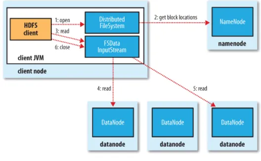
An HDFS cluster has two types of node operating in a master-worker pattern: a na-menode (the master) and a number of datanodes (workers). The namenode manages the filesystem namespace. It maintains the filesystem tree and the metadata for all the files and directories in the tree. This information is stored persistently on the local disk using two types of files: the namespace image and the edit log. It is also the namenode responsibility to know the datanodes on which all the blocks for a given file are located, however, it does not store block locations persistently, since this information is recon-structed from datanodes when the system starts.

(17)

A client accesses the filesystem on behalf of the user by communicating with the namenode and datanodes. The client presents a POSIX6_{-like filesystem interface, so the}

user code does not need to know about the details of the namenode and datanodes to work correctly.

Datanodes perform the dirty work on the filesystem. They store and retrieve blocks when they are told to (by clients or the namenode) and they report back to the namen-ode periodically with lists of blocks that they are storing.

Without the namenode, the filesystem cannot be used. In fact, if the machine run-ning the namenode goes down, all the files on the filesystem would be lost since there would be no way of knowing how to reconstruct the files from the blocks on the datan-odes. For this reason, it is important to make the namenode resilient to failure.

Figure 2.1 helps to get an idea of how the data flows between a client interacting with HDFS.

Figure 2.1: HDFS Data flow

(18)

Blocks

A disk has a block size which is the minimum amount of data that it can read or write. Filesystems for a single disk use this concept by dealing with data in blocks which are an integral multiple of the disk block size. Filesystem blocks are typically a few kilobytes in size, while disk blocks are normally 512 bytes. This is generally transparent for the filesystem user who is simply reading or writing a file. HDFS has also the concept of blocks, but it is a much larger size: 64 MB by default. Like in a filesystem for a single disk, files in HDFS are broken into block-sized chunks, which are stored as independent units. Unlike a filesystem for a single disk, a file in HDFS that is smaller than a single block does not occupy a full block’s worth of underlying storage. Having larger blocks compared to normal disc blocks minimize the cost of seeks in HDFS. By making a block large enough, the time to transfer the data from the disk can be made to be significantly larger than the time to seek to the start of the block. Thus the time to transfer a large file made of multiple blocks operates at the disk transfer rate.

Having a block abstraction for a distributed filesystem brings several benefits. First, a file can be larger than any single disk in the network. There is nothing that requires the blocks from a file to be stored on the same disk, so they can take advantage of any of the disks in the cluster. Second, making the unit of abstraction a block rather than a file simplifies the storage subsystem. The storage subsystem deals with blocks, simplifying storage management and eliminating metadata concerns. Third, blocks fit well with replication for providing fault tolerance and availability. To insure against corrupted blocks and disk and machine failure, each block is replicated to a small number of physically separate machines (typically three). If a block becomes unavailable, a copy can be read from another location in a way that is transparent to the client. When a block that is no longer available, due to corruption or machine failure, can be replicated from their alternative locations to other live machines to bring the replication factor back to the normal level.

2.2 MapReduce

MapReduce is a programming model originally designed and implemented at Google [4] as a method of solving problems that require large volumes of data using large clusters of inexpensive machines. The programming model is based on two distinct phases. A Map phase executes a function of the form M ap: (k1, v1)→list(k2, v2) that

(19)

phase aggregates the output of the mappers allowing all associated records to be pro-cessed together in the same node. The function of the Reduce phase follows the form

Reduce: (k2, list(v2))→list(v3). The transformation functions of the map and reduce

phase can be executed in parallel, keeping in mind that the execution in each node is isolated from executions in other nodes. Figure 2.2 introduces the model of a MapRe-duce execution.

Figure 2.2: Map Reduce Flow

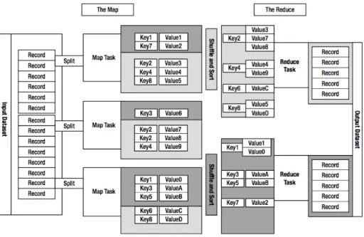
When a MapReduce job is submitted to Hadoop, the framework decomposes the job into a set of map tasks, shuﬄes, a sort and a set of reduce tasks. Hadoop is responsible for managing the distribution execution of the tasks, collect the output and report the status to the user. A typical MapReduce job in hadoop consist of the parts show in Figure 2.3.

(20)

Figure 2.3: Parts of a MapReduce job

The advantage of the programming model provided by MapReduce is that it allows the distributed execution of the map and reduce operations. When each mapping oper-ation is independent of the other, all maps can be performed in parallel, limited only by the data source and the number of CPUs available. Similarly, the reducers can perform the reduction phase in parallel. This kind of parallel execution also allows the execution to recover from a partial failure of servers or storage during the operation: if one mapper or reducer fails, the work can be rescheduled.

To achieve reliability during the execution of a MapReduce job each node is expected to report back periodically with completed work and status updates. If a node doesn’t report back for a period longer than a configurable interval, the master node marks the node as dead and distributes the node’s work to other available nodes. Reduce operations operate much the same way. Because of their inferior properties with regard to parallel operations, the master node attempts to schedule reduce operations on the same node or in the same rack as the node holding the data being operated. This property is desirable

(21)

as it reduces the bandwidth consumption across the backbone network of the datacenter.

2.2.1 A MapReduce Example

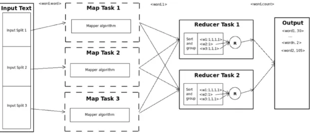
In essence MapReduce is just a way to take a big task and split it into discrete task that can be done in parallel. A simple problem that is often used to explain how MapReduce works in practice consists in counting the occurrences of single words within a text. This kind of problem can be easily solved by launching a single MapReduce job as follows.

Initially, the input text is converted into a sequence of tuples that have as key and value all the words of the text. For example, the sentence “Hello world from MapRe-duce.” is converted into 4 tuples, each of them containing one word of the sentence both as key and as value. The mapper algorithm is executed for every tuple in the input of the form <word,word>, the algorithm returns an intermediate tuple of the form <word, 1>. The key of this tuple is the word itself while 1 is an irrelevant value. After the map function has processed all the input, the intermediate tuples will be grouped together according to their key.

map( key , value ) : // key : word // value : word output . c o l l e c t ( key ,1 ) reduce ( key , i t e r a t o r v a l u e s ) : count = 0 f o r ( value in v a l u e s ) count = count + 1 output . c o l l e c t ( key , count )

Figure 2.4: Word Counter

The reduce function counts the number of tuples in the group. Because the number of tuples reflects the number of times the mappers have encountered that word in the text, the reducers output the result in a tuple of the form <word,count>. The tuples encode the number of times that a word appears in the input text. An overall picture of this particular job execution is given in Figure 2.5.

(22)

Figure 2.5: Map Reduce Example

2.3 HBase

HBase, modeled after Google’s Bigtable[5], is a distributed column-oriented database written in Java and built on top of HDFS. HBase is used on Hadoop when real time read/write random access is required in very large datasets. Although there are many products for database storage and retrieval in the market, most solutions (specially re-lational databases) are not built to handle very large datasets and distributed environ-ments. Many vendors oﬀer replication and partitioning solutions to grow the database beyond the limits of a single node but these add-ons are generally an afterthought and are complicated to install and maintain. These add-ons also add several constraints to the feature set of RDBMs. Joins, complex queries, triggers, constraints become more expensive to run or do not work at all. To avoid those problems HBase was built from the ground to scale linearly by just adding nodes to an existing cluster.

Some of the HBase features include compression, in-memory operation and filters per column basis as outlined in the original BigTable paper[5]. Tables in HBase can be used as the input and output of MapReduce jobs that run in Hadoop or could be accessed through the Java API, REST or Thrift7 _{gateway APIs.}

(23)

Figure 2.6: HBase Cluster

The scaling capabilities of HBase comes at a cost: HBase is not a relational database and doesn’t support SQL, however, given the proper problem, HBase is able to do what a RDBMS cannot: host vast amounts of data on sparsely populated tables on clusters made from commodity hardware.

2.3.1 HBase Concepts

In HBase, the data is store into labeled tables made of rows and columns. Each table cell, an intersection of a row and a column, is versioned. By default, the version field is a timestamp auto assigned by HBase when the cell is inserted. The content of all the cells is an uninterpreted array of bytes. The row key of a Table, its primary key, is also a byte array, this means that any kind of object can serve as a row key, from strings to serialized data structures. Typically all the access to the table is done via the table pri-mary key, although there are third party facilities in HBase to support secondary indexes. The row columns in an HBase table are grouped together into column families. All columns family members have a common prefix, for example, the columnsperson:name

and person:lastname are both members of theperson column family. The column fam-ilies are specified up front with the table schema definition, but new columns can be added to the column family on demand. Physically, the column family members are stored together on the filesystem.

Tables are automatically partitioned horizontally by HBase into Regions. Each re-gion compromises a subset of table’s rows. A rere-gion is defined by its first row, inclusive, and the last row, exclusive, plus a randomly generated region identifier. Initially a table

(24)

contains a single region but as the size of the region grows and after it crosses a config-urable size threshold, it splits at a row boundary into two new regions of approximately equal size. Until the first split happens, all loading will be against the single server host-ing the original region. As the table grows, the number of its regions grows. Regions are the units that get distributed over an HBase cluster. In this way, a table that is too big can be carried by a cluster of servers where each node hosts a subset of the table. Row Updates in HBase are atomic, no matter how many row columns constitute the row level transaction. This keeps the locking model simple for the user.

(25)

Chapter 3

Semantic Web and DL Concepts

This chapter focuses on presenting the main concepts related to the Semantic Web and Description Logics.

3.1 Semantic Web

The Semantic Web is an eﬀort to bring back structure to the information available on the Web by describing and linking data to establish context or semantics that adhere to defined grammar and language constructs. The structures are semantic annotations that conform a specification of the intended meaning. Therefore, the Semantic Web contains implicit knowledge often incomplete since it assumes open world semantics.

The Semantic Web addresses semantics through standardized connections to related information. This includes labeling data, unique and addressable, allowing that data to be connected to a larger context, or the web. The web oﬀers potential pathways to its definition, relationships to a conceptual hierarchy, relationships to associated in-formation and relationships to specific instances. The flexibility of a web form enables connections to all the necessary information, including logic rules. The pathways and terms form a domain vocabulary or ontology.

The flexibility and many types of Semantic Web statements allow the definition and organization of information to form rich expressions, simplify integration and sharing, enable inference of information and allow meaningful information extractions while the information remains distributed, dynamic and diverse.

(26)

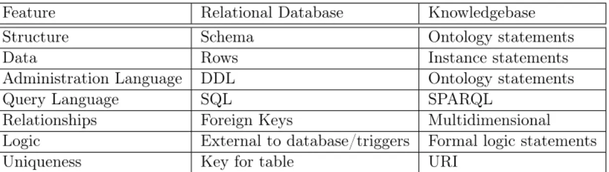
forms; knowledge bases and files. Knowledge bases oﬀer dynamic, extensible storage similar to relational databases. Files typically contain static statements. Table 3.1 compares relational databases and knowledge bases.

Feature Relational Database Knowledgebase

Structure Schema Ontology statements

Data Rows Instance statements

Administration Language DDL Ontology statements

Query Language SQL SPARQL

Relationships Foreign Keys Multidimensional Logic External to database/triggers Formal logic statements

Uniqueness Key for table URI

Table 3.1: Comparison of Relational Databases and Knowledge Bases

Relational databases depend on a schema for structure. A knowledge base depends on ontology statements to establish structure. Relational databases are limited to one kind of relationship, the foreign key. Instead, the Semantic Web offers multidimensional relationships such as inheritance, part of, associated with, and many other types, in-cluding logical relationships and constraints. An important note is that the language used to form structure and the instances themselves is the same language in knowledge bases but quite different in relational databases. Relational databases offer a different language, Data Description Language (DDL), to establish the creation of the schema. In relational databases, adding a table or column is very different from adding a row. Knowledge bases really have no parallel because the regular statements define the struc-ture or schema of the knowledge base as well as individuals or instances.

One last area to consider is the Semantic Web’s relationship with other technologies and approaches. The Semantic Web complements rather than replaces other informa-tion applicainforma-tions. It extends the existing WWW rather than competes with it, oﬀering powerful semantics that can enrich existing data sources, such as relational databases, web pages, and web services or create new semantic data sources. All types of appli-cations can benefit from the Semantic Web, including standalone desktop appliappli-cations, mission critical enterprise applications, and large scale web applications/services. The Semantic Web causes an evolution in the current Web to oﬀer richer, more meaningful interactions with information.

The Semantic Web oﬀers several languages. Rather than have one language to resolve all the information and programming needs, the Semantic Web oﬀers a range from basic

(27)

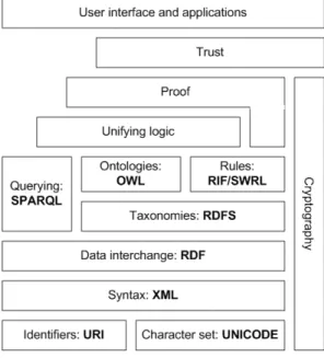
to complex. This provides Semantic Web applications with choices to balance their needs for performance, integration and expressiveness. As shown on Figure 3.1 there are some standards on top of XML that allow to express knowledge in the Semantic Web. On the Semantic Web, information is modeled primary with a set of three complementary languages: The Resource Description Framework (RDF), RDF Schema and the Web Ontology Language, OWL. RDF Defines the underlying data model and provides a foundation for the more sophisticated features of the higher levels of the Semantic Web.

Figure 3.1: The Semantic Web Stack

3.1.1 The Resource Description Framework (RDF)

RDF consist of a family of specifications from the W3C1 _{originally designed as a}

meta-data model used now as a general method for conceptual description or modeling of information that is implemented in web resources.

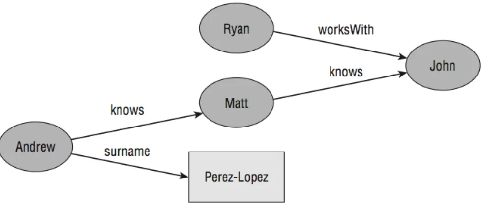
In the Semantic Web information is represented as a set of assertions called state-ments that are made up of three parts: Subject, Predicate and Object. Because of these three elements, statements are typically referred asTriples. Thesubject of a statement is the thing that the statements describes. The predicate describes a relationship between the subject and the object. Every triple can be seen as a small sentence. An example could be the triple “John plays Guitar” where John is the subject,eats is the predicate andGuitarthe object. This kind of RDF assertions form a directed graph, with subjects

(28)

and objects of each statements as nodes and predicates as edges.

Figure 3.2: A graph representation of a RDF statement

The nodes in a RDF graph are the subjects and objects of the statements that make up the graph. There are two kinds of nodes: Literals and Resources. Literals represent the concrete data values like numbers or strings and can’t be the subject of a statement, only the objects. Resources, in contrast, represent everything else; they can be either subjects or objects. Resources can represent anything that can be named. Resource names take the form of URIs (Universal Resource Identifiers). Predicates, also called

properties, represent the connections between resources; predicates are themselves re-sources. Like subjects, predicates are represented by URIs.

An RDF graph can be Serialized using multiple formats making the information rep-resented in them easy to exchange by providing a way to convert between the abstract model and a concrete format. There are several, equally expressive serialization formats. Some of the most popular are RDF/XML2_{, N3} 3_{, N-Triples}4 _{and Turtle}5_{. This means}

that depending of the application needs an RDF statement can be serialized in diﬀerent ways.

2_{http://www.w3.org/TR/rdf-syntax-grammar/} 3_{http://www.w3.org/DesignIssues/Notation3} 4_{http://www.w3.org/TR/rdf-testcases/#ntriples} 5_{http://www.w3c.org/TeamSubmission/turtle}

(29)

3.1.2 RDFS

The Resource Description Framework (RDF) provides a way to model information but does not provide a way to specify what that information means. In other words RDF cannot express semantics. To add meaning to RDF a vocabulary of predefined terms is needed to describe the information semantics. RDF Schema (RDFS) extends RDF pro-viding a language with which the users can develop shared vocabularies, that have a well understood meaning and it is used in a consistent manner to describe other resources. RDF Schema provides basic elements for the description of ontologies, otherwise called Resource Description Framework (RDF) vocabularies, intended to structure RDF re-sources.

RDFS vocabularies describe the classes of resources and properties being used in a RDF model allowing to arrange classes and properties in generalization/specialization hierarchies, define domain and range expectations for properties, assert class member-ships and specify and interpret datatypes. RDFS is one of the fundamental building blocks of ontologies in the Semantic Web and is the first step to incorporate semantics into RDF.

The list of classes defined by RDFS is shown in Table 3.2. Classes are also resources, so they are identified by URIs and can be described using properties. The members of a class are instances of classes, which is stated using the rdf:type property.

rdfs:Resource rdfs:subClassOf rdf:type rdfs:Resource rdfs:Resource rdfs:Class

rdfs:Class rdfs:Resource rdfs:Class rdfs:Literal rdfs:Resource rdfs:Class rdfs:Datatype rdfs:Class rdfs:Class rdf:XMLLiteral rdfs:Literal rdfs:Datatype

rdf:Property rdfs:Resource rdfs:Class rdf:Statement rdfs:Resource rdfs:Class rdf:List rdfs:Resource rdfs:Class rdfs:Container rdfs:Resource rdfs:Class rdf:Bag rdfs:Container rdfs:Class rdf:Seq rdfs:Container rdfs:Class rdf:Alt rdfs:Container rdfs:Class rdfs:ContainerMembershipProperty rdf:Property rdfs:Class

(30)

In RDFS a class may be an instance of a class. All resources are instances of the classrdfs:Resource. All classes are instances ofrdfs:Class and subclasses ofrdfs:Resource. All properties are instances of rdf:Property. Properties in RDFS are relations between subjects and objects in RDF triples, i.e., predicates. All properties may have defined domain and range. The Domain of a property states that any resource that has given property is an instance of the class. Range of a property states that the values of a property are instances of the class. If multiple classes are defined as the domain and range then the intersection of these classes is used. An example stating that the domain of hasSon property is Person and that the domain of the same property is Man follows:

@prefix : <http : / /www. example . org / sample . r d f s #>.

@prefix r d f s : <http : / /www. w3 . org /2000/01/ rdf−schema#>. : hasSon r d f s : domain : Person ;

r d f s : range :Man.

3.2 Web Ontology Language (OWL)

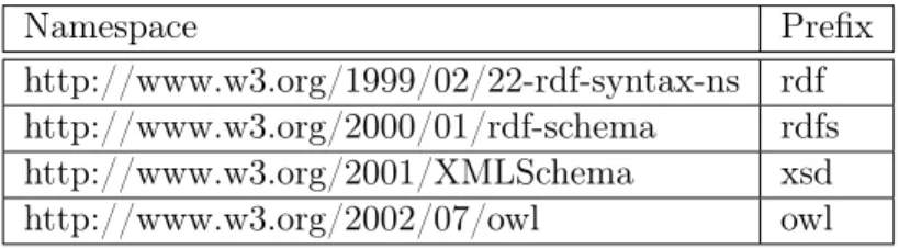
With RDF Schema it is possible to define only relations between the hierarchy of the classes and the properties or define the domain and range of these properties. The community needed a language that could be used for more complex ontologies and therefore work was done to create a richer language that would be later released as the OWL language. The Web Ontology Language (OWL) extends the RDFS vocabulary with additional resources that can be used to build more expressive ontologies for the web. OWL adds restrictions regarding the structure and contents of RDF documents in order to make processing and reasoning more computationally decidable. OWL uses the RDF and RDFS, XML Schema datatypes, and OWL namespaces. The OWL vocabulary itself is defined in the namespace http://www.w3.org/2002/07/owl and it is commonly referred to by the prefix owl. OWL 2 extends the original OWL vocabulary and reuses the same namespace. The full set of namespaces used in OWL and their associated prefixes are listed in Table 3.3.

Namespace Prefix

http://www.w3.org/1999/02/22-rdf-syntax-ns rdf http://www.w3.org/2000/01/rdf-schema rdfs http://www.w3.org/2001/XMLSchema xsd http://www.w3.org/2002/07/owl owl

(31)

Resources on the web are distributed, as a result, the resources descriptions con-tained in the Semantic Web are also distributed. OWL supports this kind of distributed knowledge base because is built on RDF, which allows you to declare and describe re-sources locally or refer to them remotely. OWL also provides a mechanism to import and reuse ontologies in a distributed environment.

3.2.1 OWL Languages and Profiles

Both the original OWL specification and OWL 2 provide profiles, or sublanguages of the language, that give up some expressiveness in exchange for computational eﬃciency. These profiles introduce a combination of modified or restricted syntax and nonstructural restrictions on the use of OWL. In the original OWL specification, there were three sublanguages:

• OWL Lite: The intention OWL Lite was to provide applications and tool devel-opers with a development target or starting point for supporting primarily classi-fication hierarchy and simple constraints. Unfortunately, OWL Lite was regarded mostly as a failure because it eliminated too many of the useful features without introducing enough of a computational benefit to make the reduced features at-tractive.

• OWL Full: OWL Full It is a pure extension of RDF. As a result, every RDF document is a valid OWL Full document, and every OWL Full document is a valid RDF document. The important point to make here is that OWL Full maintains the ability to say anything about anything. With the flexibility comes a tradeoﬀ in computational eﬃciency making OWL Full not decidable6_.

• OWL DL: OWL DL provides many of the capabilities of description logics. It contains the entire vocabulary of OWL Full but introduces the restriction that the semantics of OWL DL cannot be applied to an RDF document that treats a URI as both an individual and a class or property. This and some additional restrictions make OWL DL decidable.

With OWL 2 the main purpose of an OWL profile, as with the original OWL Languages, is to produce subsets of OWL that trade some expressivity for better computational

6_{Decidability specifies that there exists an algorithm that provides complete reasoning. It does not}

say anything about the performance of such an algorithm or whether it will complete in an acceptable or realistic amount of time

(32)

characteristics for tools and reasoners. The profiles were developed with specific user communities and implementation technologies in mind. The three standardized profiles are:

• OWL EL: The OWL EL profile is designed to provide polynomial time compu-tation for determining the consistency of an ontology and mapping individuals to classes. The relationship between ontology size and the time required to perform the operation can be represented by the formula f(x) = xa. The purpose of this

profile is to provide the expressive features of OWL that many existing large scale ontologies (from various industries) require while also eliminating unnecessary fea-tures. OWL EL is a syntactic restriction on OWL DL.

• OWL QL:The OWL QL profile is designed to enable the satisfiability of conjunc-tive queries in log-space with respect to the number of assertions in the knowledge base that is being queried. The relationship between knowledge base size and the time required to perform the operation can be represented by the function

f(a) = log(a). As with OWL EL, this profile provides polynomial time

compu-tation for determining the consistency of an ontology and mapping individuals to classes.

• OWL RL:The OWL RL profile is designed to be as expressive as possible while allowing implementation using rules and a rule processing system. Part of the design of OWL RL is that it only requires the rule processing system to support conjunctive rules. The restrictions of the profile eliminate the need for a reasoner to infer the existence of individuals that are not already known in the system, keeping reasoning deterministic.

3.3 Reasoning Basics

3.3.1 Open World Assumption

The open world assumption states that the truth of a statement is independent of whether it is known. In other words, not knowing whether a statement is explicitly true doesn’t imply that the statement is false. The closed world assumption states that any statement that is not known to be true can be assumed to be false. Under the open world assumption, new information must always be additive. It can be contradictory, but it cannot remove previously asserted information. This assumption has a significant

(33)

impact on how information is modeled an interpreted.

Most systems operate with a closed world assumption. They assume that the in-formation is complete and known. For many applications this is a safe and necessary assumption to make. However, a closed world assumption can limit the expressivity of a system in some cases because it is more diﬃcult to diﬀerentiate between incomplete information and information that is known to be false.

The open world assumption impacts the kind of inference that can be performed over the information contained in the model. In DL it means that reasoning can be performed only over information that is known. The absence of a piece of information cannot be used to infer the presence of other information.

3.3.2 No Unique Name Assumption

The distributed nature of the Semantic Web makes unrealistic to assume that everyone is using the same URI to identify a specific resource. Often a resource is described by multiple users in multiple locations and each of those users is using his or her own URI to represent the resource.

The no unique name assumption states that unless explicitly stated, it can’t be assumed that resources identified by different URIs are different. This assumption differs for the one used on traditional systems. In most database systems, all information is known and assigning and unique identifier, such a primary key, is possible. Like the open world assumption, the no unique names assumption impact inferences capabilities related to the uniqueness of resources. Redundant and ambiguous data is a common issue in information management systems, the unique names assumption makes these issues easier to handle because resources can be made the same without destroying any information or dropping and updating database records.

3.4 Description Logics

One of the reasons behind the fact that the Semantic Web community adopted Descrip-tion Logics (DL) as a core technology is that DL has been purpose of multiple studies that try to understand how constructors interact and combine to aﬀect reasoning.

(34)

that share some properties. Properties can also be specified by means of relations (roles) between individuals. The language is compositional, i.e. the concept descriptions are built by combining diﬀerent subexpressions using constructors. The semantics of the language is given in a set theoretical way over a domain which is a set of elements. A concept expression corresponds to a subset of the domain, while a role expression cor-responds to a binary relation over the domain. As their shape suggests, some of these constructors have a strong relationship with boolean operators and logical quantifiers.

A DL knowledge base consists of a terminology, TBox, and an assertional part, ABox. The TBox contains the definitions of the terms (concept definitions), while the ABox contains a set of membership and role assertions. Membership assertions relate an individual to a concept, stating that the individual involved is an instance of the concept. Role assertions state that two individuals are linked by a given role. For example:

Terminology Humans are Animals.

Women are Humans and not Male Assertions gabi is-a Human and not Male and

has a Friend who is Male

TBox Human_�Animal

W omen_�Human_{� ¬}M ale

ABox Human_{� ¬}M ale_�

∃hasF riend. M ale(gabi)

Figure 3.3: Knowledge base example

Reasoning with DL knowledge bases is a deduction process which extracts not only the facts explicitly asserted in a knowledge base but also their logical consequences. When only the terminology is involved in a deduction the reasoning is said to be Ter-minological, otherwise it is said to beHybrid.

Description Logic languages can be categorized in many diﬀerent logics, distinguished by the constructors they provides. The work done is this project is focused on ALC, considered a basis of many DL systems.

3.4.1 ALC Family of Description Logics

The language ALC consist of an alphabet of distinct concept names, role names and individual names, together with a set of constructors for building concept and role ex-pressions. Formally, a description logic knowledge base is a pairK =< T, A > whereT

(35)

is a TBox and Ais an ABox. The TBox contains a finite set of axiom assertions of the

form C _�D | C =. D , where C and D are concept expressions. Concept expressions

are of the form: A| � | ¬C|C�U|C�D| ∃R.C| ∀R.C, whereAis an atomic concept,

R is a role name, � (top or full domain) is the most general concept and ⊥ (bottom or empty set) is the least general concept. The ABox contains a finite set of assertions about individuals of the form C(a) (Concept membership assertions) and R(a, b) (Role

Membership Assertions), wherea, b are individual names.

The Semantics of description logic are defined in terms of an interpretation I =

(�I_,_�I₎_{, consisting of a nonempty domain} _�I _{and an interpretation function} _�I_{. The}

interpretation function maps concept names into subsets of the domain(AI⊆ �I₎_{, role}

names into subsets of the Cartesian product of the domain (R _{⊆ �}I _{∗ �}I₎_{, and}

indi-vidual names into elements of the domain. The only restriction on the interpretations is the unique name assumptions (UNA). Given a concept name A (or a role name R), the set denoted by AI_(or _RI_{) is called the interpretation or extension of} _A_(or_R_{) with}

respect to I.

The interpretation is extended to cover concepts built from negation (¬) , conjunction(�), disjunction(�), existential quantification(∃R.C) and universal quantification(∀R.C) as

follows: (¬C)I ₌_�I_�_CI (C_�D)I =CI_∩DI (C�D)I =CI∪DI (∃R.C)I ={x ∈ �I_|∃_{y. < x, y >}_∈_RI�_y _∈ _CI_} (∀R.C)I ₌_{_x _{∈ �}I_|∀_{y. < x, y >}_∈ _RI _→_y _∈ _CI_}

An interpretation I satisfies (entails) an inclusion axiom C _⊆D (Written I _|=C _⊆ D) if, and it satisfies an equalityC=. D ifCI =DI. It satisfies a TBox T if it satisfies

each assertion in T. The interpretation I satisfies a concept membership assertionC(a)

ifaI _∈ _CI _{and satisfies a role membership assertion}_R(a,b) _if₍_aI_{, b}I₎ _∈ _RI_. _I _satisfies

an ABoxA (I �A) if it satisfies each assertion in A. if I satisfies an axiom (or a set of

(36)

if they have the same models. Given a knowledge base K =< T, A >, the knowledge

base entails an assertionα(written(K�α)) iﬀ for every interpretation I, ifI _|=A and I |=T then I �α.

The DL ABox can be viewed as a semi-structured database, while the TBox contains a set of constraints for the data in the ABox. The TBox can be compared to data model in databases (Entity-Relationship Model in databases) but the semantic of description logics are defined in terms of interpretation diﬀerentiating them with databases. In addition, the domain of interpretation can be chosen arbitrary and it can be infinite. This, together with the open world assumption, are features that diﬀerentiate descrip-tion logics from tradidescrip-tional databases. Another particular feature of descripdescrip-tion logic is the reasoning capabilities that are associated with it. Reasoning allow to exploit the description of the model to draw conclusions about a problem.

The research community has extensively study the decidability and complexity of

ALC and its sublanguages, designing sound and complete subsumption testing algo-rithms, some extensions of ALC include:

• ALC, ALCR, ALCN R: Add number restriction concept expressions (N) and/or

role conjunction (R) toALC.

• ALCF: Add attributes (also called features), attribute composition and attribute

value map concept expressions to ALC.

• ALCF N, ALCF N R: Add number restriction expressions and role conjunction to

ALCF.

• ALCN(o): Adds role composition in number restriction expressions to ALC.

• ALC+: Adds union, composition and transitive closure role expressions to ALC.

• ALCR+: Adds transitively closed primitive roles to ALC (axioms of the form

RN _∈R+).

• ALCL:Adds a restricted form of predictive role introductions axioms toALCR+.

• T SL: Adds union, composition, identity, transitive reflexive closure and inverse

role expressions toALC.

• CIQ: Adds qualified number restriction expressions (inverse roles are the only

(37)

It is important to notice that extending the syntax of the DL language does not neces-sary increase its expressiveness. Figure 3.4 show some of the members of the ALC family.

Figure 3.4: ALC family hierarchy

3.5 Reasoning in Description Logics

A DL knowledge base support two kinds of reasoning tasks: TBox reasoning and ABox Reasoning. In TBox reasoning the basic reasoning services consist of:

• Knowledge Base Consistency: A TBox T is consistent iﬀ it is satisfiable, i.e. there is at least a non empty model forT. An interpretation I is a model for T if it satisfies every assertion inT.

• Satisfiability: AconceptC is satisfiable with respect toT if there exist a model

I of T such thatCI is nonempty. I is also a model ofC.

• Subsumption: A concept D subsumes a concept C with respect to T (C ⊆T

D or T _|= C =. D) if CI₌_DI _{for every model}_I _of_T.

• Equivalence: Two concepts C and D are equivalent with respect to T (C =.T

D or T _|= C =. D) if CI=DI for every modelI ofT.

• Disjointness: Two concept C and D are disjoint with a respect to T if for every modelI ofT,CI∩DI =θ.

(38)

Concept satisfiability is the key inference for TBox reasoning. Subsumption, equivalence and disjointness can be reduced to concept (un)satisfiability test, which can be achieved though applying the Tableau Algorithm explained on Section 3.5.1

• Subsumption: C is subsumed by D (C _⊆ D) iﬀ C_{� ¬}D is unsatisfiable with

respect to T.

• Equivalence: C and D are equivalent (C=. D) iﬀ bothC� ¬Dand D� ¬C are

unsatisfiable with respect toT.

• Disjointness: C andD are disjoint iﬀC�D is unsatisfiable with respect to T.

When reasoning in the ABox it has to be taken into consideration that there are only two kinds of assertions: concept membership assertion of the formC(a)and role membership assertion of the form R(a,b). Therefore, the ABox alone can’t be seen as a knowledge base; the ABox must be attached with its TBox. Consequently ABox reasoning will always be done with respect to its TBox. In Description Logics the basic reasoning services for ABox are:

• Instantiation Check: The problem consist to determine whether an assertion is entailed by ABox A or not (A _|= C(a)). An assertion is entailed if every

interpretation that satisfies Aalso satisfies C(a).

• Realization: Given an individual a and a set of concepts, find the most specific concept C from the set such that A|=C(a)

• Retrieval: Given an ABox A and concept C, find all individuals a such that

A_|=C(a)

• ABox Consistency: An ABoxA is consistent iﬀ it is consistent with respect to the TBox T. TBox reasoning must be used for ALC expanding the ABox with unfolded TBox concepts. An unfolded concept C’ is obtained by replacing the descriptions of the original concept with their descriptions in T. Due to the fact that C is satisfiable with respect to T iﬀ C’ is satisfiable; the original concept and the unfolded concept are equivalent,C=.T C�. Thus, the expansion ofAwith

respect to T can be obtained by replacing each concept assertion C(a) inA with the assertion C’(a). In every model of T, a concept C and its expansion C’ are interpreted in the same way. Therefore, A’ is consistent with respect toT iﬀA’ is consistent. A’ is consistent iﬀ it is satisfiable (There is at least a nonempty model for A’)

(39)

Realization and retrieval can be reduced to an instantiation test. They can be done through a series of instantiation tests. Additionally, the instantiation test can be re-duced to the consistency problem for ABox sinceA|=C(a) iﬀA∪ {¬C(a)} is inconsis-tent. Concept satisfiability can also be reduced to an ABox consistency test since C is satisfiable iﬀ {C(a)}is consistent, where a is an arbitrary individual.

3.5.1 Tableaux Algorithm

The main idea around the Tableaux algorithm is to prove the satisfiability of Concept expression D by finding a model I = (�I_,_�I₎ _{in which} _DI _�₌ _φ_{; a tableau is a graph}

which represents such model with nodes corresponding to individual and edges corre-sponding to relationships between the individuals. Typically, the algorithm starts with a single individual that satisfies D and tries to construct a complete model by inferring the existence of additional individuals or of additional constraints on the individuals. The inference mechanism consists of applying a set of expansion rules that correspond to the logical constructs of the language; the algorithm terminates either when the model is complete (no further inferences are possible) or when an obvious contradiction appears. To simplify the algorithm, the concept expression D, is assumed to be an unfolded concept expression in negation normal form (NNF). A concept is in NNF when nega-tion is applied only to concept names and not to compound terms. Arbitrary concept expression can be transformed into NNF using a the DeMorgan’s laws from Figure 3.5.

Initial Concept Equivalent Concept ¬(A�B) ¬A� ¬B

¬(A�B) ¬A� ¬B

¬¬A A

¬∀R. A ∃R.¬A

¬∃R. A _∀R._¬A

Figure 3.5: De Morgan’s rules

3.5.2 Tableaux Algorithm for ALC

The tableaux algorithm uses a tree to represent the model being constructed. Each nodex in the tree represents an individual and is labeled with a set of expression which it must satisfy: C _{∈ L}(x) _⇒ x _∈ CI_{. Each edge} _{< x, y >} _{in the tree represents a}

(40)

R=L(< x, y >⇒< x, y >∈RI).

To determine the satisfiability of a concept expression D, a tree T is initialized to contain a single nodexo, withL(x0) ={D}, the tree is expanded by continuously

apply-ing the rules from table 3.4. Tis fully expanded when none of the rules can be applied. Tcontains an obvious contradiction when, for some nodex and some conceptC,either ⊥ ∈ L(x) or _{C,_¬C_{} ⊆ L}(x).

Condtion Actions

�Rule 1. C1�C2 ∈ L(x) L(x)→ L(x)∪ {C1, C2}

2. {C1, C2}�L(x)

�Rule 1. (C1�C2) ∈ L(x) a. save T

2. {C1, C2} ∩ L(x) =Ø b. Try (x)→ L(x)∪ {C1} if, clash

restore T and try:

(x)_{→ L}(x)_{∪ {}C2}

∃Rule 1. ∃R.C _{∈ L}(x) create nodey andedge <x,y>with:

2. There is noy s.t L(< x, y >) =R and C∈ L(y) L(y)→ L(y) ∪ {C}and L(< x, y >) =R ∀Rule 1. ∀R.C ∈ L(x) L(y)→ L(y)∪ {C} There is somey s.t. L(< x, y >) =R and C /_{∈ L}(y)

Table 3.4: ALC Tableau completion rules

A fully expanded class free tree T can be converted into a model to probe the satisfiability ofD:

�I ₌_{_x_|_{x is a node in T}_}

C ={x ∈ �I_|_C _∈ _L₍_x₎_} _{for all concept names}_C _in_D

RI ₌_{_{< x, y >}_|_{< x, y > is an edge in T and}_L₍_{< x, y >}_{) =}_R_}

The algorithm is guaranteed to terminate because:

• The �,_�,_∃ rules can only be applied once to any given concept expression C in

L(x).

• The∀-rule can be applied many times to a given∀R.Cexpression in_L(x)but only

once to any given edge< x, y >.

• Applying a rule to concept expression D extends the labeling with a concept ex-pression which is always smaller than D.

(41)

The �-rule is non-deterministic and operates by performing a depth first backtracking search of the possible expansions resulting from the disjunction in D, stoping when a fully expanded tree is found or every when every possible expansion is shown to lead to a clash.

Example: Demonstrating Subsumption using Tableaux Algorithm

Given the TBox:

B =. P_{� ∀}RA D=. P _{� ∀}R.(A_�C)

The tableaux algorithm can be used to show thatB _�Dby demonstrating thatB_�¬D

is not satisfiable:

1. Unfold and normalizeB_{� ¬}D : P� ∀RA�(¬P � ∃R.(¬A� ¬C))

2. InitializeT to contain a single nodex. L(x) =_{P _{� ∀}RA_�(_¬P_{� ∃}R.(_¬A_{� ¬}C))_}

3. Apply the �-rule:

L(x)_{→ L}(x) _{∪ {}P,_∀RA,(_¬P_{� ∃}R.(_¬A_{� ¬}C))_}

4. Apply the U-rule to _¬P_{� ∃}R.(_¬A_{� ¬}C):

(a) Save Tand try: L(x)→ L(x)∪ {¬P} L(x) contains a clash: _{P,_¬P_{} ⊆ L}(x)

(b) Restore T and try: L(x)→ L(x)∪ {∃R.(¬A� ¬C)} 5. Apply the ∃-rule to ∃R.(_¬A_{� ¬}C)_{∈ L}(x):

create a new nodey and a new edge < x, y >

L(y) =_{¬A_{� ¬}C_}

L(< x, y >) =R

6. Apply the ∀-rule to ∀R.A_{∈ L}(x) and _L(< x, y >) =R:

(42)

7. Apply the �-rule to ¬A� ¬C∈ L(y):

L(y)→ L(y)∪ {¬A,¬C}

L(y) contains a clash: _{A,_¬A_{} ⊆ L}(y).

Because all the possible applications of the�-rule (step 4) have been shown to lead to a contradiction, it can be concluded that B� ¬Dis unsatisfiable, with respect to T,thus

we can say that B_�D.

3.6 Query Eﬃciency

There are two standard type of queries allowed in Description Logic: boolean queries and non boolean queries, they can respectively be seen as the instance checking and retrieval ABox reasoning services. A boolean query Qb refers to a formula of the form

Qb ←QExp, whereQExpis an assertion about an individual. For example the query:

Qb ← John : (Student� ∃takesCourse.Course) will return a boolean True or False.

Qb will returnTrue if and only if every interpretation that satisfies the knowledge base

K also satisfies QExp and return False otherwise.

A non boolean queryQnb refers to a formula of the formQnb ←QExpwhere QExp

is a concept expression. For example Qnb ←Student� ∃takesCourse.Course. In this

case, the query will return one of the members of the set{⊥, M_},where_⊥refers to the

empty set andM represent a set of models that satisfiesQExp with respect to the knowl-edge baseK.A non boolean query is trivially transformed into a set of boolean queries. Answering a boolean query consist in resolving an entailment problem. For example, answering Qb ← John : (Student� ∃takesCourse.Course) can be resolved by

check-ing K _|= John: (Student_{� ∃}takesCourse.Course). Thus, boolean query or instance

checking can be reduce to knowledge base satisfiability: K _|= C(a) iﬀ K_{∪ {¬}C(a)_} is

unsatisfiable.

As explained before, many DL reasoners can deal with very expressive languages, however, when the reasoning has to be performed on large ABoxes, scaling problem ap-pear. The main reasons for this problem is that the reasoners must compute the tableau algorithm, mainly using main memory and the fact that some of the Tableau algorithms require a lot of CPU power to run.

(43)

3.6.1 Retrieval Optimization using the Pseudo model technique

In order to avoid the need to run the completion of a Tableau model for every can-didate individual in the ABox, the first optimization that comes to mind is to detect the obvious instances of a conceptC. [10] introduces such a method. The advantage of this technique is that reduces the number satisfiability tests executed during the query answering process. The pseudo model technique introduces a very eﬀective mergeable test which reuses information computed from previous satisfiability tests.

Each subsumption test (C⊆D) can be transformed into a satisfiability testunsat(C� ¬D). IfC_{� ¬}Dis satisfied thenC�D. In order to check if the conjunctionC_{� ¬}Dis

satisfiable or not, a mergeable test between C’s pseudo model and ¬D’s pseudo model

can be applied. If there is not interaction between the pseudo models of C and ¬D,

thenC_{� ¬}D is satisfied. Therefore,C�D.

The pseudo model technique is sound but it is not complete. This means that if the pseudo models of C and ¬D cannot be merged, the completion of the Tableau model

must be complete to test the satisfiability ofC� ¬D. However, using the mergeable test

can eﬀectively reduce the number of individual tests, reducing the number oft times the Tableau algorithm needs to run.

3.6.1.1 Flat pseudo models for ABox Reasoning

To realize an individual a, given the concepts D1...Dn, it is required to perform a set

of ABox consistency tests for ADi=A∪ {¬Di(a)}.The main purpose of the flat pseudo

model technique is to provide an eﬃcient sound mergeable test for an individuala and sets of concept terms¬Di.

Pseudo model for an individual a

Assuming that the ABoxAis consistent and there exists a non-empty set of completions

C. let A� _∈ C. The pseudo model M for the individual a in A is defined as the tuple < MA, M¬A, M∃, M∀>w.r.t A’ and A using the following definitions:

MA₌_{_A_|_a_:_{A � A}�_}

M¬A={A|a:¬A � A�}

M∃=_{R_|a:_∃R.C � A�_} M∀={R|a:∀R.C � A�}

(44)

Pseudo model for a concept D

Similarly the pseudo model for a concept D can be defined as follow. Given the set

LA(a) defined as the set of concept terms from all concept assertions for a in a

com-pleted ABox A’. Let D be a concept andA the ABox A=D(a), the pseudo model M

for D consists of the sets:

M_DA={D|D � LA(a)}

M_D¬A=_{D_{| ¬}D � LA(a)}

M_DA={R | ∃R.C � LA(a)}

M_DA=_{R _{| ∀}R.C � LA(a)}

The mergeable test for the flat pseudo models M1 and M2 consist in checking

whether there are interactions between the models by checking for atomic concepts:

((MA1

D ∩M¬AD2 �= φ)∨(MDA2 ∩M¬AD1 �= φ)) and for roles successors: ((M∃AR1 ∩M∀AR2 �=

φ)_∨(MA2

∃R∩M∀AR1 �=φ)).

The pseudo model can be used before the TBox subsumption or the ABox satisfia-bility test for an individual and a concept. For example, to test whether D is the type of individual a, it is suﬃcient to test whethera’s pseudo model is mergeable with ¬D’s

pseudo model, if they are mergeable then D is not the type of individual a.

3.6.2 Soundness and Completeness

A procedure is sound when there are no wrong inferences drawn from the knowledge base using the procedure. A sound procedure may fail to find solutions in some cases, even though they exist. A procedure is complete if its execution can obtain all the correct inferences from the knowledge base. A complete procedure may find solutions when there are actually no solutions. In other words, if the procedure is sound, and the answer found is aﬃrmative, the answer can be trusted. On the other hand, if the procedure is complete, and the answer is negative, then the answer can be trusted.

There are many sound and incomplete algorithms which are considered as good ap-proximation to resolve a problem because they can simplify the procedure to find a solution reducing the computational complexity. The pseudo model technique is one of these algorithms. Therefore, when the mergeable test is applied to resolve the sub-sumption of C1 �C2, beingC1 and C2 complex concept expressions and the following