Wavelet-Based Compressive Sensing for Point Scatterers
Gregory WILSENACH
1, Amit Kumar MISHRA
2 1Department of Mathematics, University of Cambridge, UK.2Department of Electrical Engineering, University of Cape Town, South Africa.
Abstract. Compressive Sensing (CS) allows for the sam-pling of signals at well below the Nyquist rate but does so, usually, at the cost of the suppression of lower amplitude sig-nal components. Recent work suggests that important infor-mation essential for recognizing targets in the radar context is contained in the side-lobes as well, which are often sup-pressed by CS. In this paper we extend existing techniques and introduce new techniques both for improving the accu-racy of CS reconstructions and for improving the separa-bility of scenes reconstructed using CS. We investigate the Discrete Wavelet Transform (DWT), and show how the use of the DWT as a representation basis may improve the ac-curacy of reconstruction generally. Moreover, we introduce the concept of using multiple wavelet-based reconstructions of a scene, given only a single physical observation, to derive reconstructions that surpass even the best wavelet-based CS reconstructions. Lastly, we specifically consider the effect of the wavelet-based reconstruction on classification. This is done indirectly by comparing outputs of different algo-rithms using a variety of separability measures. We show that various wavelet-based CS reconstructions are substan-tially better than conventional CS approaches at inducing (or preserving) separability, and hence may be more useful in classification applications.
Keywords
Compressive sensing, wavelet, radar, reconstruction, sparse scenes, filtering, point scatterers
1. Introduction
Compressive Sensing (CS) is a powerful new frame-work that provides methods for approximate reconstruction of signals using a number of samples far below that given by the Nyquist criteria. The approximate reconstruction con-tains only the highest energy components of the original signal, with all other components effectively discarded. In the radar domain, CS has been shown to be a useful tech-nique for sensing different types of scenes that are often very sparse, and in which low energy components (e.g. side-lobes) are often undesirable. The use of CS in reducing the sampling rate, and thus the associated hardware/software
complexity, of radars has been dealt with in many recent publications (e.g. [1, 2]). CS has also been shown to be use-ful in applications to other areas of radar, including speckle reduction [3] and classification [4].
How effectively a given scene can be reconstructed us-ing CS depends largely on two important choices, namely, the choice of the sensing matrix, which determines the wave-forms used to sense the scene, and the representation ba-sis, the basis in which the scene is expressed. In particu-lar, the accuracy of the CS reconstruction depends on choos-ing a representation basis such that the scene is sparse when expressed in that basis and is incoherent with the sensing matrix (details on incoherence are included below). In this paper we discuss the effectiveness of the Discrete Wavelet Transform (DWT) as a representation basis.
It should be noted that the use of the DWT as a repre-sentation basis for CS reconstruction is not a new idea. The application of wavelet-based CS to Synthetic Aperture Radar (SAR) has been discussed in other papers (e.g [5–8]) and there has also been work done on the application of wavelet-based CS to images (e.g. [9–11]). In this paper we take a dif-ferent approach to studying wavelet-based CS, focusing on a vastly different type of scene and considering classifica-tion needs. We primarily work with scenes that consist of only a single scattering center. We consider such a limita-tion acceptable for the following three reasons. Firstly, such scenes, or linear combinations of such scenes, are very com-mon in practice (e.g. planes on a blank sky) and are often used in to model SAR scenes, where the scene is modeled using a few dominating scattering centers [12]. Secondly, as discussed in recent work [13], classification of some SAR targets, and many targets sensed using low-resolution radar, is improved when we include side-lobe information usually suppressed by CS. Thirdly, side-lobe information is partic-ularly hard for CS to preserve, given that the importance of a particular component of a scene for classification may not be dependent on energy, and so may be suppressed by CS despite its importance.
There are many novelties in the current work. First of all, we test the effectiveness of CS and wavelet-based CS in reconstructing such single-scatter scenes. We also introduce the concept of combining wavelet-based CS reconstructions, all of which can be built from a single observation, in or-der to build a signal reconstruction more accurately than any wavelet-based CS reconstruction. Lastly, we consider the
fect of CS and wavelet-based CS reconstruction on the clas-sifiability of a scene, discussing how wavelet-based CS and CS affect separability measures and general classification ef-forts.
The rest of the paper is organized as follows. Section 2 gives a brief background to compressive sensing. Section 3 expounds the Radar model that we have used and some of the implementation steps for our experiments. Section 4 describes the way we have simulated and reconstructed the scenes. In Section 5, we describe the algorithm for using multiple representations. Section 6 elaborates our exper-iments on classification and the use of CS, and Section 7 concludes the work and discusses some open questions and limitations of the current work.
2. Compressive Sensing Background
This section includes a brief introduction to CS as well as some basic notations used in this paper. The CS intro-duction included here is based on a tutorial by Cand`es [14]. We make use of some of the informal language found in [14]. For a more technical explanation of this language please read the cited paper. For the sake of brevity, in this paper we will refer to CS using the DWT with some wavelet as the representation basis as ‘wavelet-based CS’ and CS using the identity as just ‘CS’ or ‘identity CS’.
Suppose some scene can be represented by some vector
x∈Rn. We note that for any representation basis (i.e.
orthog-onal matrix)Ψ, we may expandxin that basis byx=Ψθ, whereθ∈Rn. We say thatxhas a sparse representation if
the coefficient vectorθis sparse.
Suppose now we haveN sensing waveformsφn, n= 1,2, . . . ,N, which can be rewritten in matrix notation as Φ= [φ1,φ2, . . . ,φN]T such that Φ is an orthogonal matrix, often refereed to as the sensing basis or sensing matrix. The act of sensingxwith this matrix can then be summarized as
y=Φx=ΦΨθ, (1)
whereyis the output of the sensing process. In this sce-nario reconstructingxfromyis trivial, as we can simply in-vert the orthogonal matrixΦ. In CS we instead do not use all the sensing waveforms in order to sense the scene. In-stead we choose someM waveforms from{φ1,φ2, . . . ,φN}, whereM<N, and form an incompleteM×Nsensing ma-trix denoted by ˜Φ. The act of sensing the scene can thus be summarized by
y=Φ˜x=ΦΨθ˜ =Aθ, (2)
whereyis now an M length vector and A=ΦΨ˜ . In this case the inverse problem is ill-posed. The great insight of CS theory is that despite this fact, the scene can be approxi-mately reconstructed supposing that sensing and tion bases are sufficiently incoherent and that the representa-tion basis induces a sufficiently sparse representarepresenta-tion of our
scenex. We now explain these terms. We say that a scenex
has anS-sparse representation inΨif the coefficient vectorθ has at mostSnon-zero components. Furthermore, we define the coherence between a sensing basis and a representation basisµ(Φ,Ψ), as given by [14] µ(Φ,Ψ) =√N· max 1≤k,j≤N φk,ψj, (3)
whereφkis a row inΦandψjis a column inΨ. Informally, we may understand coherence as a measure of the degree to which the rows ofΦprovide a sparse representation of the columns ofΨ, and the other way around [15]. We say two such bases are incoherent if their coherence is low (closer to 1) and coherent if it is high (closer to√N).
2.1 Undersampling and Reconstruction
The degree to which these high sparsity and incoher-ence properties are met, determine the level of undersam-pling which will still result in accurate signal reconstruction. The reconstruction of the signal is achieved by solving the optimization problem: min ˜ θ∈RN θ˜ ` 1 subject to y= ˜ ΦΨθ.˜ (4)
The output of the optimization problem provides us some es-timate for the vectorθ, which we denote by ˆθ. We retrieve our estimate for the vectorx, denoted by ˆx, using:
ˆ
x=Ψθ.ˆ (5)
The required number of samples for accurate reconstruction,
M, is determined by the following inequality:
M≥C·µ(Φ,Ψ)2·S·log(N/δ), (6)
whereµdenotes coherence,Sdenotes sparsity andδdenotes a chosen constant to determine the chance of accurate recon-struction (the chance of accurate reconrecon-struction is given by 1−δ). The positive constantCcan usually be taken to be less then 10, estimations of this constant are included in [14].
2.2 Restricted Isometry Property and Noise
For practical purposes CS needs to remain effective even if the signal is only approximately sparse or if noise is introduced. In order to solve this problem we need to un-derstand the Restricted Isometry Property (RIP) which is an alternate condition for accurate signal recovery. We define the RIP as follows: for eachS∈ {1,2...}we define the isom-etry constantδSof a matrixAto be the smallest number such that (1−δS)kθk2` 2≤ kAθk 2 `2 ≤(1+δS)kθk 2 `2 (7)holds for any arbitrary S-sparse vector θ. We may say, loosely, that the RIP is obeyed forSifδSis not close to one. We also note that the RIP offers a measure of how closely
Using the RIP we now consider the case when noise is introduced into our system. In this we may think of the CS sensing operation as being given by
y=Φ˜x+z, (8)
wherezrepresents a random variable introduced to account for noise or system inaccuracies, and ˜Φ is our M×N CS sensing matrix.
We consider then the adjusted optimization program: min ˜ θ∈RN θ˜ ` 1 subject to y−ΦΨ˜ θ˜ ` 2≤ε, (9)
where the noise in the system is bounded by someε. Simi-larly the success of reconstruction using these relaxed opti-mization constraints is determined by the restricted isometry property, details can be found in [14].
We say that ifA=ΦΨ˜ obeys the RIP and we have that δ2S<
√
2−1, then we have that the solution to (9), denoted by ˆθ, obeys θˆ−θ ` 2 ≤C0kθ−θSk`1/ √ S+εC1, (10)
whereC0andC1are constants andθSis the signalθbut with all but theSlargest amplitude components set to zero.
This result establishes that CS is a robust and practical system capable of acting on noisy and imperfect signals, i.e. those that appear in real-life application. Moreover, this re-sult does not assume thatθisS-sparse, and tells us that ifθis notS-sparse, then it is as though the algorithm knew ahead of time which where the highestS components of the sig-nal and measured those directly [14]. We utilize this result in that we explicitly consider noisy and otherwise imperfect signals in this paper.
2.3 Dantzig Selector
It has been shown that similar reconstruction algo-rithms based on the Dantzig selector can also be very effec-tive in the noisy case [16]. In particular, this Dantzig selector based reconstruction has been shown to be quite effective in Radar applications [3], and as such will be used in all exper-iments in this paper unless stated otherwise. The Dantzig se-lector based reconstruction uses the following optimization:
min ˜ θ∈RN θ˜ `1 subject to A∗(Aθ˜−y) `∞ ≤ γ, (11)
whereγis a user-defined value andA∗(Ax˜−y)is a measure of how well the residual and each column ofAcorrelate [3].
3. Radar Model and Implementation
In this section we discuss our implementation of CS and our choice of sensing matrix. We employ a very simi-lar implementation and sensing matrix to the one outlined by Ender for compatibility with pulse compression [1].
3.1 Radar and Sensing Basis
In order to conveniently apply CS-theory to a given scene we have to first consider a quantization of the space in that scene. We do this by assuming that all scatterers ap-pear in some range interval[rmin,rmax]and then breaking that interval up intoNdistinct points. It can be noted here that this is not the most accurate model for radar targets. How-ever this is an acceptable model which directly follows from the scattering center model which is an often used model in radar imaging. In this way we have that theith element of the lengthNscene vector corresponds to a distance of
ri=rmin+ (i−1)
rmax−rmin
(N−1) . (12) In this section, whenever a distance is given, we assume that the distance is given by one of these discrete points, i.e. if we have some distancerthen we have thatr∈ {r1,r2. . .rN}. Rather than using conventional radar sensing wave-forms, e.g. a chirp, we instead construct our sensing basis usingN distinct frequencies represented by the wave num-bers k1,k2. . .kN. In order to enforce orthogonality of the sensing waveforms used, we define this sequence of wave numbers by
kl=k0+j
4π
r2−r1
. (13)
It can be noted here that, this way of representation, even though unconventional, is not novel. It resembles to the stepped frequency type radar waveforms. Now, if we ig-nore the Doppler effect, we have that the normalized return signal of some target after being sensed with the frequency associated with the wave numberklis given by
sl(r) =e−j2klr. (14)
We can now represent the arbitrary scene sensed with the frequency associated with the wave numberkjas
yl= N
∑
i=1 aisl(ri) = N∑
i=1 aie−j2klri, (15)whereyl is the return, and ai is the complex amplitude as-sociated with the scatterer atri. From this equation, if we think of(a1,a2, . . .aN)as our scene vector, we have that the sensing waveforms are given by
φi= 1
√
N(s1(ri),s2(ri), . . . ,sN(ri)∀i∈ {1, . . .N}. (16)
We can now construct the sensing matrix by selecting just
M<Nof these sensing waveforms. This matrix is given by Φli= (sv(l)(ri)),∀l∈ {1. . .M},∀i∈ {1, . . .N}, (17)
where the function vselects the waves used in sensing, in this paper we always use uniform selection. It is worth not-ing that the matrix in (17) is of course a simplification over a real world sensing matrix. A brief discussion of the extent of this simplification and its relationship to real world sens-ing matrices, as well as how much this simplification effects CS testing, may be found in [1].
(a) The first scene
(b) The second scene
(c) The third scene
Fig. 1.The three simulated scenes used in this paper.
3.2 Computing the Reconstruction
In order to compute the CS reconstruction we need to be able to find a solution to a given optimization problem. In this paper we have used the Dantzig selector, solving the op-timization problem using the primal-dual algorithm. In our implementation, this requires rewriting the (in general) com-plex matrices and vectors used above in (8) in terms of real entries. We denote these versions of the sensing matrixA, the scene vectorxand the noise vectorzbyA∗,x∗andz∗ re-spectively. A similar change is also introduced by Ender [1]. We define the real versions of these components by
A∗= ℜ(A) −ℑ(A) ℑ(A) ℜ(A) x∗= ℜ(x) ℑ(x) z∗= ℜ(z) ℑ(z) . (18) This gives us the vectory∗, where:
y∗=A∗x∗+z∗. (19)
The effect of considering these real versions is that all these matrices have had their rows and column counts doubled, and the vectors have had their row count doubled, which cor-responds to a doubling of the effectiveMandNvalues used for reconstruction. These matrices can now be used to com-pute the signal reconstruction of ˆxusing the Dantzig selector:
ˆ x∗= Re(xˆ) Im(xˆ) , (20)
from which we construct ˆx, the complex reconstruction ofx. In other papers using`1minimization as part of CS (see [1] for an explicit construction) similar adjustments have been made. However, since we are using the primal-dual algo-rithm, rather than the simplex algoalgo-rithm, there is no require-ment that the reconstructed vector be positive, as in [1]. This is a positive change as such a requirement would require us to double the number of columns in the matrix use for re-construction, thus reducing the effectiveness of CS. As it stands, this implementation does require doubling the effec-tiveM andN values. However, given that the dependence onNin Cand`es inequality (see (6)) is sub-linear, we expect a doubling of N to require less than a doubling of the re-quiredM. As such, although we make these changes in order to overcome difficulties with the reconstruction algorithm, these changes should in fact result in a better reconstruction.
However, there is a potential negative effect which should be noted. By decoupling the real and imaginary com-ponents of a signal the possibility arises that the optimiza-tion algorithm may negate only the real or imaginary part of a signal at a particular index, thus distorting the recon-struction [1]. Although this distortion is perhaps potentially problematic, it has not been found to be noticeably damaging in any of the experiments discussed in this paper. Ender [1] uses a similar method, and also notes that this method is stan-dard.
4. Simulation and Reconstruction
In this section we test the effectiveness of CS, that is CS reconstruction using the identity matrix as the represen-tation basis, and contrast it with wavelet-based CS, that is CS reconstruction using the DWT with some wavelet as the representation basis. As discussed above we have selected to discuss scenes consisting of only a single scattering center. The fact that such scenes, and sums of such scenes, are very common both in lower resolution radar and SAR, combined with the fact that information contained in the sidelobes in such scenes have been shown to be important for classifica-tion efforts, has made the study of means to preserve such scenes important.
We now consider three simulations of such scenes, each containing only a single target. In the first scene the target is just a single metal plate, in the second scene the target con-sists of two cylinders and two spheres and in the third scene the target consists of three corner reflectors and a cylinder. In each case the target is shrunk down until it is entirely con-tained within a single resolution cell. The scenes are simu-lated using an environment built using the parametric model described in [12]. These scenes are complex and their very sparse nature makes useful visualization challenging, how-ever we have included a log graph of the absolute value of each scene in Fig. 1.
With regard to the sensing matrix, we use the matrix in-troduced in (17) as the sensing matrix in all CS and wavelet-based CS reconstructions. It is worth noting that the (quired) use of a particular sensing matrix separates our re-sults from those that come from image-based tests, in which
0 50 100 150 200 250 300 350 400 0 0.5 1 1.5 2 2.5 3 3.5
number of sensing waveforms used (M value)
av er ag e eu cl id ea n di st an ce b et w ee n re co ns tr uc ti on an d or ig in al sc en e Identity Daubechies 4 Wavelet (a) Daubechies 4 0 50 100 150 200 250 300 350 400 0 0.5 1 1.5 2 2.5 3 3.5
number of sensing waveforms used (M value)
av er ag e eu cl id ea n di st an ce b et w ee n re co ns tr uc ti on an d or ig in al sc en e Indentity Haar Wavelet (b) Haar 0 50 100 150 200 250 300 350 400 0 0.5 1 1.5 2 2.5 3 3.5
number of sensing waveforms used (M value)
av er ag e eu cl id ea n di st an ce b et w ee n re co ns tr uc ti on an d or ig in al sc en e Identity Simlet 6 Wavelet (c) Symlets 6 0 50 100 150 200 250 300 350 400 0 0.5 1 1.5 2 2.5 3 3.5
number of sensing waveforms used (M value)
av er ag e eu cl id ea n di st an ce b et w ee n re co ns tr uc ti on an d or ig in al sc en e Identity Coiflet 3 Wavelet (d) Coiflets 3
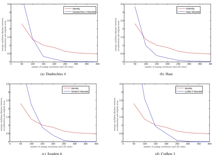
Fig. 2.Each graph shows the average euclidean distance over the three scenes between the wavelet-based CS reconstructions and the original scenes for varyingMvalues.
very convenient sensing matrices may be chosen. In all of these experiments unless otherwise stated we useN=1024 andM =200. All DWT matrices were constructed using Matlab’s single-level discrete wavelet transform.
4.1 Reconstruction with Wavelets
We took the scenes depicted in Fig. 1 and reconstructed them using identity CS and wavelet-based CS. In particu-lar, we reconstructed these scenes using wavelets from the Daubechies, Symlets and Coiflets families as well as using a number of Biorthogonal wavelets. In our experiments we found that the Daubechies-4 DWT had the most effective representation basis, followed by the Haar DWT. For more detail on these wavelets the reader may wish to consult any standard text on wavelet analysis, e.g. [17].
In Fig. 2 we have summarized representative results from this experiment using four graphs, one for each of a small number of wavelets, with each graph showing how the accuracy of the identity based CS reconstruction com-pares with the wavelet-based CS reconstruction as we vary theMvalue.
Since the only signal information contained in these scenes is contained in the side-lobes, Fig. 2 acts to
demon-strate just how much better the wavelet-based reconstruc-tions are at preserving side-lobe information. As seen in the figure, this is especially true as we increase theM value, with the identity CS reconstruction converging considerably slower than the wavelet reconstruction in each case.
There are two points we should make regarding these simulations and experiments. Firstly, although Fig. 2 is con-structed using averages over the three scenes, in fact almost exactly the same set of graphs was produced when we con-sidered each scene individually (rather than together, as an average). Second, it is important to note that, excepting very lowMvalues, we do not see one wavelet-based reconstruc-tion improving beyond another as we increase theMvalue; a reconstructions stays either above or below as we increase
M. This note is needed in order to make sense of our conclu-sion that Daubechies-4 DWT was the most ‘effective’ DWT representation matrix tested.
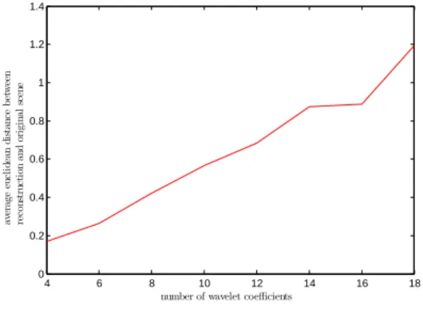
It is important to note that Fig. 2 acts only to give a cross-section of our results from this investigation into the application of the DWT as a CS representation basis. Fur-ther study was done on the Daubechies wavelet family and the closely related Symlet family. We analyzed how the effectiveness of the reconstruction is affected by the num-ber of coefficients (and vanishing moments) of the given
wavelet. The results of this investigation have been summa-rized in Fig. 3, which shows the Euclidean distance between the Daubechies reconstruction and the original scene for a varying number of wavelet coefficients. From this figure we can see that as we increase the number of coefficients (and thus vanishing moments), the wavelet-based CS reconstruc-tion decreases in accuracy substantially. Similar results were found when investigating the Symlet family.
4 6 8 10 12 14 16 18 0 0.2 0.4 0.6 0.8 1 1.2 1.4
number of wavelet coefficients
av er ag e eu cl id ea n di st an ce b et w ee n re co ns tr uc ti on an d or ig in al sc en e
Fig. 3.The average Euclidean distance (over the three scenes) between the wavelet-based CS reconstruction and the original scene using wavelets from the Daubechies series with a varying number of wavelet coefficients.
4.2 Noise and Reliability
Since we are discussing the accurate reconstruction of the side-lobes of point scatterers, which are often lower en-ergy components, the adverse effect of noise may be partic-ularly troubling. In Tab. 1 we compare the CS reconstruc-tion and the Daubechies-4 wavelet-based CS reconstrucreconstruc-tion for differing signal to noise ratios (SNR’s), usingM=150,
N=1024 and the same three scenes as above.
SNR 10 dB 20 dB 30 dB 40 dB 50 dB
wavelet-based CS 8.81 3.54 1.32 0.60 0.24
CS 8.19 3.16 1.39 1.01 0.93
Tab. 1.The average Euclidean distance between each of the CS reconstructions and the original scenes with noise for different SNR values and the average Euclidean distance between each of the Daubechies-4 based CS reconstruc-tions and the original scenes with noise for different SNR’s.
From the table we can see that Daubechies-4 is ro-bust with respect to noise beyond 20 dB, below which the wavelet-based reconstruction starts to degenerate and pro-duces reconstructions less accurate than the those produced by the identity CS reconstruction. The behavior of the Daubechies-4 wavelet is not unusual with respect to noise, and our experiments with other wavelet-based CS recon-structions have produced very similar tables.
5. Combining Multiple
Reconstruc-tions
When reconstructing a signal using CS it is possible to do it using multiple representation matrices. In this way we may be able to, having only physically sensed a scene once, construct multiple ‘views’ of the same scene. We now make two observations, firstly, the noise and inaccuracies as a result of the CS reconstruction vary for different sensing matrices (this is easy to see and has been confirmed thor-oughly in our own investigation) and secondly, the noise in the scene is ‘moved around’ when we reconstruct using dif-ferent representation bases.
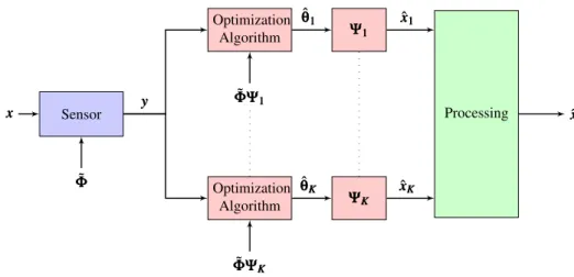
These two observations suggest the possibility of pro-ducing a better reconstruction by considering multiple views of the same scene, each constructed with a different rep-resentation matrix, and then using the different informa-tion contained in each reconstrucinforma-tion to produce a final, im-proved, scene reconstruction. We have summarized this gen-eral approach in Fig. 4.
This method of reconstruction is very generally defined so far, as clearly there are multiple ways a set of reconstruc-tions may be combined or analyzed in order to produce an improved final reconstruction. Moreover, the availability or efficacy of such methods may depend on the sensing envi-ronment or other practical limitations inherent in the sensing context. Given the broad set of possible algorithms for com-bining multiple wavelets, and the broad set of contexts in which such methods could be applied, we have limited our-selves to considering quite simple, but broadly applicable, methods of combining reconstructions. Our introduction and discussion of these methods should act to provide evidence of the utility of the general approach and as a starting point for further research on more sophisticated methods.
In this paper we consider two methods of recon-struction: The Voting method and Deviation Thresholding method. These methods are discussed in the following sec-tions.
5.1 The Voting Method
In brief, the Voting algorithm constructs a final (or out-put) reconstruction from multiple reconstructions by taking some token reconstruction (hopefully one we know to be ac-curate) and then removing those parts of the reconstruction that fluctuate in sign between reconstructions (the thought being that such components are most likely just noise).
More formally, given some scene vector of lengthn, we begin by producing multiple reconstructions of that scene using a number of different (sparsity inducing) represen-tation matrices, as in Fig. 4. A particular reconstruction, called the reference reconstruction vector, and a numberV, called the voting threshold, are both chosen. For every
i∈ {1, . . . ,n}, we construct a numberCi, which is the number of reconstruction vectors with a positiveith element minus
xxx Sensor ˜ Φ ΦΦ Processing xxxˆ Optimization Algorithm ˜ Φ Φ ΦΨΨΨ111 Ψ Ψ Ψ111 Optimization Algorithm ˜ Φ Φ ΦΨΨΨKKK Ψ Ψ ΨKKK ˆ θ θ θ111 xxxˆ111 yyy ˆ θ θ θKKK xxxˆKKK
Fig. 4.An overview of the system for combining CS reconstructions.
the number of reconstructions with a negativeith element. If|Ci|<V, then theith of of the reference reconstruction is set to be zero. If instead|Ci| ≥V, then theith element of the reference reconstruction is unaltered. The output recon-struction is the (now edited) reference reconrecon-struction.
In order to test this method we used the same three scenes discussed in earlier parts of this paper. We simu-lated these scenes using N=1024 and sensed them using
M=150. We used fifteen different wavelets; including the even Daubechies series, and a number of Symlet and Coiflet wavelets. All DWT matrices were constructed using Mat-lab’s single-level discrete wavelet transform.
We chose the Daubechies-4 wavelet-based CS recon-struction to be the reference reconrecon-struction, as it proved to be the most accurate reconstruction in our trials, and imple-mented the voting method using a voting threshold of 10 (i.e. requiring a majority of 66% of the reconstructions to agree on the sign of an element). The results of the simulation can be seen in Tab. 2. For example the first entry in the table shows that the Euclidean distance between the actual scene and the reconstructed scene for the first example (Scene 1) is 0.32 when using Daubechies-4 wavelet based CS.
Sc1 Sc2 Sc3
Daubechies-4 CS 0.32 0.44 0.30 Voting Method 0.39 0.48 0.37
Tab. 2.The Euclidean distance between the reconstruction of each scene and the original scene using both the Daubechies-4 wavelet-based CS reconstruction and the voting method reconstruction.
From Tab. 2 we can see that by combining the wavelet based reconstructions using the voting method we could im-prove on the accuracy of the Daubechies-4 wavelet-based CS reconstruction by an average of 15%. We again note that the Daubechies-4 wavelet-based CS reconstruction is the most accurate reconstruction we have found, and so this
repre-sents a substantial improvement. Moreover, we tested this scenario using different noise levels. As expected, while the accuracy of the reconstructions produced by both methods deteriorated with the introduction of noise, the combined re-construction deteriorated much slower, as some of the noise was canceled by the voting method.
5.2 Deviation Thresholding
In brief, the Deviation Thresholding algorithm con-structs a final (or output) reconstruction from multiple re-constructions by taking some token reconstruction and then removing all those components which vary ‘too much’ be-tween reconstructions.
More formally, given some scene vector of lengthn, we begin by producing multiple reconstructions of that scene us-ing a number of different (sparsity inducus-ing) representation matrices. We again fix a reference vector and chose a value
T, known as the threshold.
This method is slightly more sophisticated than the vot-ing method described above. We again begin reconstructvot-ing a given scene vector by choosing a particular reconstruction as our reference reconstruction and a thresholdT. For ev-ery i∈ {1, . . . ,n}, we compute the standard deviation and the mean of the set consisting of theith elements of the re-construction vectors, which we denote byσi, andµi respec-tively. If|σi/µi|>T, then theith element of the reference reconstruction is set to zero, if|σi/µi| ≤T, thenith element of the reference reconstruction is unchanged. The output re-construction is the (now edited) reference rere-construction.
We tested this method of combining reconstructions us-ing the same experiment we used to test the Votus-ing method. The deviation method produced results that where not as strong, improving on the Daubechies-4 reconstruction by an average of 5%.
Sc1 Sc2 Sc3 Sc1 0 1.63 2.71 Sc2 1.63 0 1.19 Sc3 2.71 1.19 0 1 Sc1 Sc2 Sc3 Sc1 0 1.93 2.41 Sc2 1.93 0 1.05 Sc3 2.41 1.05 0 1 Sc1 Sc2 Sc3 Sc1 0 4.32 7.28 Sc2 4.32 0 2.96 Sc3 7.28 2.96 0 1
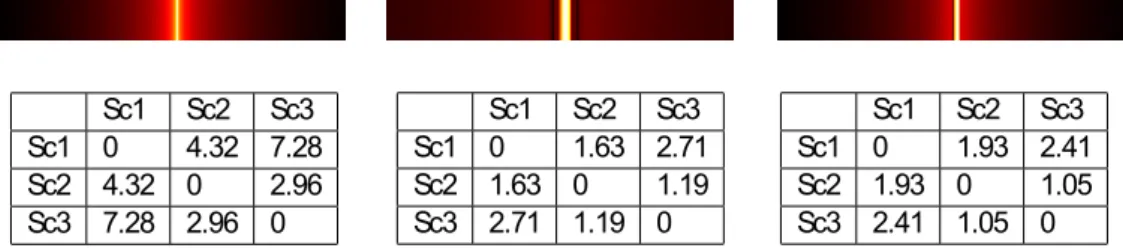
Fig. 5.The effect of windowing on the euclidean distance between the scenes. We show the distances between the scenes without any windowing effect (left) and the distances between the scenes after windowing with the Nuttall window (middle) and the Hamming window (right). In each case we include a log graph of the amplitude of the first scene showing the effect of the window.
5.3 Choosing a Reference Reconstruction
In the above two methods we have made use of a ref-erence reconstruction. The idea is that the refref-erence recon-struction acts as the ‘default’ reconrecon-struction, that we then al-ter using knowledge from the other reconstructions we have available. We have used a reference reconstruction partly be-cause it makes it easy to see the improvement that using mul-tiple reconstructions has over just a single reconstruction. While in some scenarios, e.g. when the properties of a likely scene are known a priori, it may be possible to intelligently select an appropriate reference reconstruction in practice. In other cases it may not be known which representation matrix corresponds to the most accurate reconstruction. In that case the above methods may still be used, given some automatic way of generating an ‘appropriate’ reference reconstruction. As an aside, we investigated two methods for doing so, one in which we took the reference reconstruction to be the mean of the reconstructions and one in which we took the reference vector to be that one with the lowest average dis-tance to all other vectors. In both cases no significant dif-ferences were observed in the results of either of the above methods.6. Signal Separability and
Classifica-tion
In conventional radar applications, e.g. airplanes against a sky, it is not uncommon for a target to fit into a sin-gle resolution cell. In that case, it may not be possible to classify the target using only the high energy components and it may be necessary to consider classification informa-tion contained in the side-lobes [13]. We sought to test this hypothesis and considered the same three scenes used in this paper thus far, each containing one target in a single reso-lution cell. We found that many standard schemes for sup-pressing side-lobes, including various windowing functions, have the effect of reducing the (Euclidean) distance between scenes; thus making the scenes harder to distinguish and so making classification more difficult. Results from this ex-periment have been summarized in Fig. 5. We also found that the Bhattacharyya Distance, details of which are in-cluded below, also decreased with the suppression of side-lobes, which indicated an increase in the upper bound on the
Bayes error. Further work on the effect of side-lobe suppres-sion on classification has been discussed in [13], including a discussion on how more sophisticated side-lobe reduction schemes, including nonlinear apodization [18] and refined nonlinear apodization [19], can also have a negative effect on classification.
Since side-lobes are often suppressed in the prepro-cessing stage [13], an apparent advantage of CS is its sup-pression of low-energy components, and thus side-lobes. As such, this approach of preserving side-lobe information may seem fundamentally counterproductive to a major advantage of the CS reconstruction. In this section we present evi-dence supporting the effectiveness of CS, and, in particular wavelet-based CS, in preserving side-lobe information and hence improving classification. In particular we show how, given a choice of wavelet, the use of the DWT helps preserve the separability of the scenes with respect to the Euclidean metric and, furthermore, that it lowers the upper bound on classification error.
6.1 Classification Using a Single Wavelet
In order to show how well the wavelet-based CS recon-struction preserves side-lobe information we simulated three scenes and applied appropriate classification measures. We used the same three scenes as in the previous parts of this paper. These scenes were sensed and reconstructed usingN=512,M=80 and SNR=30 dB. We rotated the targets in each of these scenes through 15 degrees in both direc-tions in increments of 0.06 degrees, creating three clusters of observations, each representing a particular class. We then sensed and reconstructed these scenes using wavelet-based CS and identity CS. These two reconstruction schemes sim-ilarly produced three clusters of observations, and simsim-ilarly we estimated the distributions associated with these classes. We then compared these classes for the original scenes, the CS reconstruction and the wavelet-based CS reconstruction, using two different measures of separability.
First, we used the average Euclidean distance between scenes. This measure is given in (21) for two clusters of ob-servations A and B, where all obob-servations are vectors inRN.
dist(A,B) = 1
This Euclidean measure, although somewhat simplistic, con-veys some information regarding the separability of the clus-ters and indicates the effectiveness of the nearest neighbor classification algorithms. In Tab. 3 we have included the average Euclidean distance between the original scenes, the CS reconstructed scenes and the wavelet-based CS recon-structed scenes.
Sc1 vs. Sc2 Sc2 vs. Sc3 Sc1 vs. Sc3
Perfect 21.64 10.57 24.35
Identity CS 20.54 9.85 22.34
Haar CS 20.76 10.18 23.46
Tab. 3.The average euclidean distance between each pair of clusters (one cluster for each scene) supposing perfect reconstruction, CS reconstruction using the identity rep-resentation matrix and CS reconstruction using the Haar wavelet.
From Tab. 3 we can see that indeed the Haar wavelet based CS reconstruction is more effective at inducing separabil-ity than conventional CS with respect to this measure. It is worth noting that the DWT is an orthogonal transform and so an isometry in Euclidean space. Thus it would make no difference if we were to consider the output of the CS op-timization algorithm, denoted by ˆθin (5), or the complete wavelet-based CS reconstruction, denoted by ˆxin (5), the distance between the clusters would still be the same.
The Euclidean metric does not do a good job of taking into account the variance (or covariance, for more than one dimension) of each of these distributions, which is important when considering classifiability. As such, we use the Bhat-tacharyya distance, which does take into account covariance and acts as an important statistical measure of the separabil-ity of two distributions [20, 21]. If we assumed that each of our three classes can be modeled as a multivariate normal distribution, we may estimate the covariance matrices and means of the distributions associated with the classes. The Bhattacharyya distance can then be calculated using (22), whereX1 andX2 are two classes or distributions with the means given byX1andX2and covariance matrices given by Σ1andΣ2. DB(X1,X2) = 1 8 X1−X2 T Σ1+Σ2 2 −1 X1−X2 +1 2log detΣ1+Σ2 2 p det(Σ1)det(Σ2) . (22)
The Bhattacharyya distance is equal to the optimum Cher-noff distance whenΣ1=Σ2 [20]. The Bhattacharyya dis-tance is particularly important as it can be used to calculate the Bhattacharyya bound. For simplicity, we only consider the Bhattacharyya bound between two classes. The Bhat-tacharyya bound is denoted byεµ, and is defined in (23).
εµ(X1,X2) =0.5e−DB(X1,X2) (23)
We note that the covariance matrices of any two classes in this simulation are approximately equal. As such, the Bhat-tacharyya distance is approximately equal to the optimum Chernoff distance, and the Bhattacharyya bound is approx-imately equal to the Chernoff bound [20]. Thus the Bhat-tacharyya bound gives us an estimate for an upper bound on the Bayes error between any two classes. In Tab. 4 we show the Bhattacharyya bound for each pair of classes given perfect reconstruction, CS reconstruction and wavelet-based (Haar) CS reconstruction.
Sc1 vs. Sc2 Sc2 vs. Sc3 Sc1 vs. Sc3
Perfect 0.058 0.032 0.031
Identity CS 0.056 0.039 0.041
Haar CS 0.057 0.032 0.031
Tab. 4.The Bhattacharyya bound calculated for each pair of classes supposing perfect reconstruction, identity CS re-construction and Haar wavelet CS rere-construction.
From Tab. 4 we can see that the Haar wavelet-based CS reconstruction results in a Bhattacharyya bounds very similar to those expected if we had perfect reconstruction, and actually slightly improves upon the perfect reconstruc-tion in some cases. Furthermore, the comparing identity and Haar CS reconstructions in Tab. 4, we can see that the wavelet-based CS reconstruction results in lower Bhat-tacharyya bounds than those produced using the CS recon-structed scenes.
It is interesting to note the contrast in behavior between the Bhattacharyya bound and the average Euclidean distance as measures of separation. Comparing Tab. 3, for the Eu-clidean measure, with Tab. 4, for the Bhattacharyya bounds, we can see that that the wavelet-based CS reconstructed classes appear less separable than the original scene classes. However, when we begin to consider the covariance matrices associated with each class, the classifiability of the wavelet-based reconstruction improves dramatically when compared with the classes constructed from the original scenes. Com-bined with the fact that the wavelet-based reconstruction is also inaccurate, we can conclude that although the wavelet reconstruction moves the clusters closer together and pro-duces less than perfect reconstructions, the wavelet recon-structions are less scattered, which makes up for the accu-racy loss and thus produces Bhattacharyya bounds compara-ble to those for the original scene classes.
It is worth noting an important difference between clas-sification and reconstruction. When testing reconstruction we found that the Daubechies-4 wavelet-based CS produced the most accurate reconstruction. Naturally, the ability to re-construct accurately is related to our ability to classify the scene. However, we note that the Haar wavelet-based recon-struction, which we found to be only the second most accu-rate wavelet for CS reconstruction wavelet, in fact outper-forms the Daubechies-4 with respect to the above two clas-sification measures.
7. Conclusions
In this paper we discussed the importance of the wavelet transform based CS in three important respects: firstly, as a representation basis for increasing the accuracy of CS reconstructions for a particularly important and com-mon class of scene; secondly, for developing new tools with which to even further increase the accuracy of CS recon-struction and, thirdly, to improve the ability of CS to retain important classification information found in side-lobes.
Scenes consisting of some number of point scatters are common, both in low resolution radar and when modeling SAR images. It has been shown, both here and in cited works, that the classification of such scenes depends on our ability to accurately sense the side-lobes. This poses a po-tential problem for CS, a recent discovery in sensing which has the dubious advantage of suppressing side-lobes. In this paper we have discussed the DWT as a potential solution to this problem. We have shown that the DWT, particularly the Daubechies-4 DWT, can be very effective in accurately re-constructing such scenes. We have briefly discussed how the wavelet-based CS reconstruction begins to deteriorate as we increase the number of coefficients/vanishing points. Given the susceptibility of side-lobes to even low levels SNR’s, we tested our wavelet-based CS reconstruction with differing noise levels, finding it deteriorated reasonably quickly but remained more accurate than CS until deteriorating at SNR at around 20 dB.
In this paper we also introduced a novel idea for im-proving CS reconstructions by taking multiple reconstruc-tions with respect to differing representation bases. We in-troduced two different methods of combining these multiple reconstructions, the Vote Method and the Deviation Thresh-olding method. We tested these methods and found that, us-ing the DWT for a number of different wavelets as our set of representation bases, that we could further improve upon the best wavelet-based CS reconstructions by more than 15% using only the simplest, unoptimized methods.
Lastly, we discussed how the use of the DWT as a rep-resentation basis can greatly improve the ability of CS to preserve classification information contained in side-lobes. In order to judge classifiability we considered two measures of separability between classes: a measure based on the av-erage Euclidean distance between members of classes and the Bhattacharyya bound. We found that the Haar wavelet-based reconstruction was very effective, lowering the Bhat-tacharyya bound to slightly below what we would expect if we had perfect reconstruction.
7.1 Limitations and Open Questions
In this paper no serious attempts where made to opti-mize the selection of a wavelet for wavelet-based CS recon-struction. There is work here in constructing wavelets, or showing no construction possible, that may dramatically im-prove upon the constructions using these standard wavelets.
Further work needs to be done on the effect of separating the imaginary and real components.
The approach of combining multiple CS reconstruc-tions remains largely unexplored. Can we infer a good reconstruction from its relationship with other reconstruc-tions? For example, a good reconstruction may have a lower average Euclidean distance to the other reconstructions. Can we use parts of different reconstructions by looking for pieces which appear natural (e.g. do not have sharp edges) and combine those pieces to form an improved reconstruc-tion? Similarly in the Voting method the voting threshold is heuristically chosen. However it can be noted that changing the threshold will make the reconstruction better at the cost of more demanding computation.
In classifiability there are a number of interesting ques-tions. Can multiple reconstructions produce better results for classification? Could we, for instance, combine the probabil-ities of a number of probabilistic classifiers, each of which is run on a different reconstruction of the same scene, and improve results?
The above discussions will be our future research di-rections.
References
[1] ENDER, J. On compressive sensing applied to radar. Sig-nal Processing, 2010, vol. 90, no. 5, p. 1402–1414. DOI: 10.1016/j.sigpro.2009.11.009
[2] TELLO, M., LOPEZ-DEKKER, P., MALLORQUI, J. J. A novel strategy for radar imaging based on compressive sensing. IEEE Transactions on Geoscience and Remote Sensing, 2010, vol. 48, no. 12, p. 4285–4295. DOI: 10.1109/TGRS.2010.2051231 [3] MANN, S., PHOGAT, R., MISHRA, A. K. Dantzig selector based
compressive sensing for radar image enhancement. In2010 Annual IEEE India Conference (INDICON). Kolkata (India), 2010, p. 1–4. DOI: 10.1109/INDCON.2010.5712730
[4] MISHRA, A. K., WILSENACH, G., INGGS, M. Information sens-ing for radar target classification ussens-ing compressive senssens-ing. In 13th International Radar Symposium (IRS). Warsaw (Poland), 2012, p. 326–330. DOI: 10.1109/IRS.2012.6233371
[5] SI, X., JIAO, L., YU, H., et al. SAR images reconstruction based on compressive sensing. In2nd Asian-Pacific Conference on Synthetic Aperture Radar (APSAR). Xian (China), 2009, p. 1056–1059. DOI: 10.1109/APSAR.2009.5374210
[6] CHEN, H., WAN, Q., FAN, R. Beampattern synthesis using reweighted l1-norm minimization and array orientation diversity. Ra-dioengineering, 2011, vol. 22, no. 2, p. 602–609.
[7] HERMAN, M. A., STROHMER, T. High-resolution radar via com-pressed sensing. IEEE Transactions on Signal Processing, 2009, vol. 57, no. 6, p. 2275–2284. DOI: 10.1109/TSP.2009.2014277 [8] BHATTACHARYA, S., BLUMENSATH, T., MULGREW, B., et al.
Fast encoding of synthetic aperture radar raw data using compressed sensing. InProceedings of the 2007 IEEE/SP 14th Workshop on Sta-tistical Signal Processing. Washington DC (USA), 2007, p. 448–452. DOI: 10.1109/SSP.2007.4301298
[9] YANG, S., ZHANG, Z., DU, H., et al. The compressive sensing based on biorthogonal wavelet basis. InProceedings of the 2010 In-ternational Symposium on Intelligence Information Processing and Trusted Computing. Washington, DC (USA), 2010, p. 479-482. DOI: 10.1109/IPTC.2010.146
[10] BI, X., CHEN, X., ZHANG, Y., et al. Image compressed sensing based on wavelet transform in contourlet domain. Sig-nal Processing, 2011, vol. 91, no. 5, p. 1085–1092. DOI: 10.1016/j.sigpro.2010.10.006
[11] XIAO, J., YANG, H., LUO, W. Compressed sensing by wavelet-based contourlet transform. InProceedings of the 2011 International Conference of Information Technology, Computer Engineering and Management Sciences. Washington, DC (USA), 2011, vol. 3, p. 75– 78. DOI: 10.1109/ICM.2011.165
[12] GERRY, M. J., POTTER, L. C., GUPTA, I. J., et al. A parametric model for synthetic aperture radar measurements.IEEE Transactions on Antennas and Propagation, 1999, vol. 47, no. 7, p. 1179–1188. DOI: 10.1109/8.785750
[13] BAKER, C., INGGS, M., MISHRA, A. Waveform processing-domain diversity and ATR. In19th European Signal Processing Con-ference (EUSIPCO 2011). Barcelona (Spain), 2011, p. 431–435.
[14] CANDES, E. J., WALKIN, M. B. An introduction to compressive sampling.IEEE Singal Processing Magazine, 2008, vol. 25, no. 2, p. 21–30. DOI: 10.1109/MSP.2007.914731
[15] BARANIUK, R., STEEGHS, P. Compressive radar imaging. In IEEE Radar Conference. Boston (USA), 2007, p. 128–133. DOI: 10.1109/RADAR.2007.374203
[16] CANDES, E. J., TAO, T. Near-optimal signal recovery from ran-dom projections: universal encoding strategies.IEEE Transactions on Information Theory, 2006, vol. 52, no. 12, p. 5406–5425. DOI: 10.1109/TIT.2006.885507
[17] MALLAT, S. A Wavelet Tour of Signal Processing: The Sparse Way. 3rd ed. Burlington (USA): Academic Press, 2008. ISBN: 0123743702
[18] STANKWITZ, H. C., DALLAIRE, R. J., FIENUP, J. R. Nonlin-ear apodization for sidelobe control in SAR imagery.IEEE Trans-actions on Aerospace and Electronic Systems, 1995, vol. 31, no. 1, p. 267–279. DOI: 10.1109/7.366309
[19] PANIGRAHI, R. K., MISHRA, A. K. A novel algorithm for apodiza-tion and super-resoluapodiza-tion in Fourier imaging. In2011 International Conference on Devices and Communications (ICDeCom). Mesra (In-dia), 2011, p. 1–5. DOI: 10.1109/ICDECOM.2011.5738468 [20] FUKUNAGA, K.Introduction to Statistical Pattern Recognition. 2nd
ed. San Diego (USA): Academic Press, 1990. ISBN: 0122698517 [21] MISHRA, A. K. Separability indices and their use in radar signal
based target recognition.IEICE Electronics Express, 2009, vol. 6, no. 14, p. 1000–1005. DOI: 10.1587/elex.6.1000
About Authors . . .
Gregory WILSENACHgraduated from the department of Electrical Engineering, University of Cape Town in 2011 and the faculty of Mathematics at the University of Cambridge in 2014. He is currently working towards his PhD in mathemat-ical logic at the University of Cambridge.
Amit Kumar MISHRAgraduated from Regional Engineer-ing College Rourkela, India in 2001. After workEngineer-ing for one year each in Defence R&D Organization, India and Wipro Technologies, Bangalore, he started his graduation studies in the University of Edinburgh in 2003. He joined Indian Institute of Technology Guwahati, as an Assistant Professor in 2006, where he was an academic till 2011, after which he joined the University of Cape Town. His main areas of interest are Radar information processing and pattern recog-nition. He is a Senior Member of IEEE since 2013 and a Y rated researcher in South Africa. He was the recipient of IRSI Young Scientist Award for year 2008 and Endeavor Research Fellowship in 2010.