UC Santa Cruz Previously Published Works
Title
Point-biserial correlation: Interval estimation, hypothesis testing,
meta-analysis, and sample size determination.
Permalink
https://escholarship.org/uc/item/3h82b18b
Author
Bonett, Douglas G
Publication Date
2019-09-30
DOI
10.1111/bmsp.12189
Peer reviewed
eScholarship.org
Powered by the California Digital Library
British Journal of Mathematical and Statistical Psychology (2019) ©2019 The British Psychological Society
www.wileyonlinelibrary.com
Point-biserial correlation: Interval estimation,
hypothesis testing, meta-analysis, and sample size
determination
Douglas G. Bonett
*
Department of Psychology, University of California, Santa Cruz, California, USA
The point-biserial correlation is a commonly used measure of effect size in two-group designs. New estimators of point-biserial correlation are derived from different forms of a standardized mean difference. Point-biserial correlations are defined for designs with either fixed or random group sample sizes and can accommodate unequal variances. Confidence intervals and standard errors for the point-biserial correlation estimators are derived from the sampling distributions for pooled-variance and separate-variance versions of a standardized mean difference. The proposed point-biserial confidence intervals can be used to conduct directional two-sided tests, equivalence tests, directional non-equivalence tests, and non-inferiority tests. A confidence interval for an average point-biserial correlation in meta-analysis applications performs substantially better than the currently used methods. Sample size formulas for estimating a point-biserial correlation with desired precision and testing a point-biserial correlation with desired power are proposed. R functions are provided that can be used to compute the proposed confidence intervals and sample size formulas.1. Introduction
The independent-samplest-test is widely used in psychological research to compare two population means that have been estimated from two independent samples. It is common practice to report the results of an independent-samplest-test as ‘significant’ or ‘non-significant’. Of course, a ‘significant’ result does not imply that any practical or scientifically important difference in population means has been detected, and a ‘non-significant’ result should not be interpreted as evidence of a true null hypothesis. The latest edition of thePublication Manual of the American Psychological Association
states that ‘effect sizes and confidence intervals are the minimum expectations for all APA journals’ (American Psychological Association, 2010, p. 33). Point and interval estimates of Cohen’s d or the point-biserial correlation are recommended supplements to an independent-samplest-test (see, for example, Kline, 2013). The point-biserial correlation also is used in psychometric item analyses to assess the association between an item-deleted total score and a dichotomous item score (Crocker & Algina, 1986; Lord & Novick, 1968).
Some researchers prefer the point-biserial correlation as a measure of effect size in a two-group design over Cohen’sd because of its familiar correlation metric (McGrath
*Correspondence should be addressed to Douglas G. Bonett, Department of Psychology, University of California, Santa Cruz, CA 95064, USA (email: [email protected]).
& Meyer, 2006). Cohen’s d is also difficult to interpret if the response variable is not normally distributed (Bonett, 2009). McGrath and Meyer (2006) provide a detailed comparison of Cohen’sd and the classical point-biserial correlation and conclude that neither measure is universally superior. A neutral stance regarding a preference for Cohen’sd or the point-biserial correlation is taken here. The purpose of this paper is to present alternative measures of point-biserial correlation, develop a variety of confidence intervals for point-biserial correlations, explain how the proposed confidence intervals can be used to test different types of hypotheses regarding point-biserial correlations, and develop sample size formulas that can be used to design a study to estimate a point-biserial correlation with desired precision or conduct a point-biserial hypothesis test with desired power.
2. Three types of standardized mean differences
A point-biserial correlation can be defined in terms of a standardized mean difference. Three types of standardized mean differences are described here. One type is appropriate for both experimental and non-experimental designs if equal population variances can be assumed; a second type is appropriate for non-experimental designs and does not assume equal population variances; and a third type is appropriate for experimental designs and does not assume equal population variances. In an experimental design with two treatments, a simple random sample is obtained from some population of sizeNand the sample is then randomly divided into two groups (not necessarily of equal sizes) where one group receives treatment A and the other group receives treatment B. In an experimental design, the sample sizes in each treatment condition are assumed to be fixed. In a non-experimental design, two types of sampling methods are common. With simple random sampling, a random sample is obtained from some population of sizeNand the members of the random sample are classified into two groups on the basis of some existing characteristic (e.g., male or female). With simple random sampling in a non-experimental design, the total sample size is fixed and the group sample sizes are random. With stratified random sampling, the population of size N is stratified into two subpopulations of sizesN1andN2on the basis of some existing characteristic. A random
sample is then taken from each of the two subpopulations. With stratified random sampling the two sample sizes need not be equal and are assumed to be fixed.
LetXbe a dichotomous variable with values 1 and 2. The values ofXrepresent the two treatment conditions in an experimental design or the two subpopulations in a non-experimental design. LetYdenote a quantitative response variable. The most common type of standardized mean difference is defined as
d1¼
l1l2
ð Þ
r ; ð1Þ
where ljis the population mean of Yat X= j andris an assumed common standard
deviation ofYat each level ofX. If the homoscedasticity assumption can be justified,d1is appropriate for both experimental and non-experimental designs.
Now consider a two-group non-experimental design where p is the proportion of members in the population that belong to subpopulation 1 and 1–pis the proportion of members in the population that belong to subpopulation 2. The variance of Y for all members of the population can be decomposed into between-group and within-group
variances where the within-group variance is pr2
1þð1pÞr 2
2. This suggests the standardized mean difference
d2¼ l1l2 ð Þ ffiffiffiffiffiffiffiffiffiffiffiffiffiffiffiffiffiffiffiffiffiffiffiffiffiffiffiffiffiffiffiffiffi pr2 1þð1pÞr22 p ; ð2Þ
which is appropriate for non-experimental designs and does not assume homoscedas-ticity. Note that ifr2
1¼r 2
2thend2reduces tod1.
A third type of standardized mean difference that does not assume homoscedasticity is defined as d3¼ l1l2 ð Þ ffiffiffiffiffiffiffiffiffiffiffiffiffiffiffiffiffiffiffiffiffiffiffiffi ðr2 1þr22Þ=2 p ; ð3Þ
and is appropriate for experimental designs where participants are randomly assigned to treatment conditions. In a two-group experiment,ljandr2j are respectively the mean and
variance ofY, assuming all members of the population had received treatmentj.Given that
r2
1 and r22 describe the same population in an experimental design, the unweighted average of these two variances is an appropriate description of the average within-treatment variance. Note that ifr2
1 = r22thend3reduces tod1.
Estimators ofdi(i= 1, 2, 3) will be used to define different estimators of point-biserial
correlation. A frequently used estimator ofd1, sometimes referred to as Cohen’sd, is ^ d1¼ ^ l1l^2 ð Þ ^ rp ; ð4Þ where^rp¼ ffiffiffiffiffiffiffiffiffiffiffiffiffiffiffiffiffiffiffiffiffiffiffiffiffiffiffiffiffiffiffiffiffiffiffiffiffiffiffiffiffiffiffiffiffiffiffiffiffiffiffiffiffiffiffiffiffiffiffiffi n11 ð Þr^2 1þðn21Þ^r22 ½ =df p
,njis the sample size atX = j,df = n1+n2–2, ^
r2
j is the unbiased estimator of the population variance ofYatX = j, andl^jis the sample
mean ofYatX= j.The estimatorr^2
phas two uses. It is an optimal estimator of a common
variance and also a consistent estimator ofpr2
1þð1pÞr 2
2in non-experimental designs when simple random sampling is used.
The following estimator of d2 is appropriate in non-experimental designs with
stratified random sampling wherepis known:
^ d2¼ ð^ l1l^2Þ ffiffiffiffiffiffiffiffiffiffiffiffiffiffiffiffiffiffiffiffiffiffiffiffiffiffiffiffiffiffiffiffiffi pr^2 1þ ð1pÞ^r22 p ; ð5Þ
and does not assume homoscedasticity. An estimator of d3, which is appropriate in
experimental designs and does not assume homoscedasticity (Bonett, 2009), is
^ d3¼ ^ l1l^2 ð Þ ffiffiffiffiffiffiffiffiffiffiffiffiffiffiffiffiffiffiffiffiffiffiffiffi ðr^2 1þr^22Þ=2 p : ð6Þ
3. Alternative measures of point-biserial correlation
If homoscedasticity can be assumed, one type of population point-biserial correlation for non-experimental designs can be defined in terms ofd1as
q1¼ d1 ffiffiffiffiffiffiffiffiffiffiffiffiffiffiffiffiffiffiffiffiffi d2 1þpð11pÞ q ; ð7Þ
wherepis the proportion of members in the population that belong to subpopulation 1. If homoscedasticity can be assumed, a second type of population point-biserial correlation for experimental designs can be defined in terms ofd1as.
q2¼
d1 ffiffiffiffiffiffiffiffiffiffiffiffiffi
d21þ4
q ; ð8Þ
wherepis set to 1/2 to reflect the fact that the entire population could hypothetically be assessed under one treatment condition and thesamepopulation could also be assessed under a second treatment condition.
A third type of population point-biserial correlation, which does not assume homoscedasticity, can be defined in terms ofd2as
q3¼ d2 ffiffiffiffiffiffiffiffiffiffiffiffiffiffiffiffiffiffiffiffiffi d22þ 1 pð1pÞ q ; ð9Þ
and is appropriate for non-experimental designs. A fourth type of population point-biserial correlation, which does not assume homoscedasticity, can be defined in terms of
d2as
q4¼ ffiffiffiffiffiffiffiffiffiffiffiffiffid3
d23þ4
q ; ð10Þ
and is appropriate for experimental designs. Note thatq3is a heteroscedastic alternative to
q1 and q4 is a heteroscedastic alternative to q2. With homoscedasticity, q1 = q3 and
q2= q4.
If the dichotomous variableXis a nominal scale measurement of some attribute (e.g., male versus female or treatment A versus treatment B), the sign of the point-biserial correlation depends on how the two groups are coded and only the absolute magnitude of the point-biserial provides useful information. However, ifXrepresents an ordinal scale measurement of some attribute (e.g., control versus treatment or 1 week of treatment versus 3 weeks of treatment), then both the sign and the magnitude of the point-biserial correlation provide useful information.
In a single-factor between-subjects design, another popular measure of effect size is g2¼1r2=r2
Y, where r
2 is an assumed common variance of Y within each level
of the between-subjects factor, and r2
Y is the variance of Y. g
2 describes the proportion of the response-variable variance that is predictable from the independent variable. In a two-group non-experimental design, r2
Y is the variance of Y for all
members in the population andg2can be defined asq2
1. In a two-group experimental design, r2 Y ¼r 2þ ðl 1l2Þ 2=
4 (McGrath & Meyer, 2006). In an experimental design
g2 can be defined as q2 2:
Some references claim that a point-biserial correlation has a range from–1 to 1 (Stuart, Ord, & Arnold, 1999, p. 496) while other references (see, for example, Lord & Novick,
1968, p. 340) claim that the point-biserial correlation has a maximum of about .8. Given thatdiis unbounded, it is clear thatqihas a range of–1 to 1. Althoughqihas a theoretical
range of–1 to 1, the values ofq1andq3depend on the values ofp. Table 1 gives the values ofq1corresponding to different values ofd1forp = .1, .3, and .5. The entries in Table 1 suggest that a ‘large’ point-biserial correlation is smaller than what might be considered to be a ‘large’ Pearson correlation between two quantitative variables.
The claim that a point-biserial correlation has a maximum value of about .8 applies to the case whereYandXare bivariate normal andXhas been artificially dichotomized. In this situation, it can be shown (Gradstein, 1986) that the classical point-biserial correlation has a maximum value of about .8 and that this maximum is achieved atp = 1/2. IfXhas been artificially dichotomized, then a biserial correlation is usually a more appropriate measure of association than a point-biserial correlation (Stuartet al., 1999, p. 492).
4. Independence and mean-independence
For two quantitative variables X and Y, a Pearson correlation equal to 0 implies independence ofXandYonly in the special case of bivariate normality. For the point-biserial correlations defined here, what doesqi = 0 (i =1,. . ., 4) imply? To answer this
question, letYandXrepresent two random variables and letrandsbe positive integers. Goldberger (1991) shows thatYis independent ofXifE(XrYS) = E(Xr)E(YS) for allrands,
Yis mean-independent ofXifE(XrY)= E(Xr)E(Y) for allr, andYandXare uncorrelated if
E(XY) = E(X)E(Y), assuming these expectations exist. Goldberger also shows that mean-independence impliesE(Y|X) = E(Y) for allX. Consequently, ifl1= l2thenYis
mean-independent ofX. Henceqi = 0 (i= 1,. . ., 4) implies thatYis mean-independent ofXfor
any distribution ofYthat has a finite mean and variance. Furthermore,qi = 0 (i =1,. . ., 4)
implies thatYis independent ofXfor any distribution ofYif the shape of the distribution ofYis the same at each level ofX.
5. Point-biserial estimators
The estimators of a population standardized mean difference given in Section 2 can be used to define estimators ofqi(i= 1,. . ., 4). Pearson’s classical estimator ofq1can be
expressed as (Hays, 1988, p. 311)
Table 1. Values ofq1as a function ofd1andp
d1 p =.5 p=.3 p =.1 0 0 0 0 0.2 .10 .09 .06 0.5 .24 .22 .15 1.0 .45 .42 .29 1.5 .60 .57 .41 2.0 .71 .68 .51 2.5 .78 .75 .60 3.0 .83 .81 .67
Note. q1=q3with homoscedasticity,q1 =q2withp=.5, andq1=q4with homoscedasticity and p=.5.
^ q1¼ t ffiffiffiffiffiffiffiffiffiffiffiffiffiffiffi t2þdf p ; ð11Þ wheret¼ð^l1^l2Þ= ffiffiffiffiffiffiffiffiffiffiffiffiffiffiffiffiffiffiffiffiffiffiffiffiffiffiffiffiffiffiffiffiffiffi ^ r2 pð1=n1þ1=n2Þ q
;df¼n1þn22, and^r2pis the pooled variance
estimate used in equation (4). After some algebra, equation (11) can be expressed as
^ q1¼ ^ d1 ffiffiffiffiffiffiffiffiffiffiffiffiffiffiffiffiffiffiffiffiffiffiffi ^ d2 1þ df np^ð1^pÞ q ; ð12Þ
wheren = n1+n2and^p¼n1=n. In meta-analysis applications, the following estimator of
q1is typically used: q1¼ c^d1 ffiffiffiffiffiffiffiffiffiffiffiffiffiffiffiffiffiffiffiffiffiffiffiffiffiffi c2^d2 1þ^pð11^pÞ q ; ð13Þ
wherec =1–3/(4n–9) is a bias adjustment to^d1derived by Hedges (1981). The following estimator ofq2is defined using^d1:
^ q2¼ ^ d1 ffiffiffiffiffiffiffiffiffiffiffiffiffi ^ d2 1þ4 q : ð14Þ
It does not assume homoscedasticity and is appropriate in experimental designs with equal or unequal sample sizes. Ifpis known and stratified random sampling is used, the following estimator ofq3is defined using^d2:
^ q3¼ ffiffiffiffiffiffiffiffiffiffiffiffiffiffiffiffiffiffiffiffiffi^d2 ^ d22þ 1 pð1pÞ q : ð15Þ
It does not assume homoscedasticity.
The following estimator of q4, which is appropriate for experimental designs with equal or unequal sample sizes and does not assume homoscedasticity, is defined using^d3:
^
q4¼ ffiffiffiffiffiffiffiffiffiffiffiffiffi^d3
^ d23þ4
q : ð16Þ
To summarize, the classical point-biserial estimator (q^1) is appropriate in both experimental and non-experimental designs if homoscedasticity can be assumed. The classical estimator also is appropriate in non-experimental designs with heteroscedastic-ity if simple random sampling is used so thatp^will be a consistent estimator ofp. The estimator^q2is appropriate in experimental designs with equal or unequal sample sizes if homoscedasticity can be assumed, while^q4is appropriate in experimental designs with equal or unequal sample sizes when homoscedasticity cannot be assumed. The estimator
^
q3is appropriate in non-experimental designs with equal or unequal sample sizes when homoscedasticity cannot be assumed and stratified random sampling has been used.
6. Bias of point-biserial correlation estimators
The small-sample bias of ^q1 andq1 is given in Table 2 for a non-experimental design with simple random samples of size n = 30 and n = 60, three values ofp (.20, .35, .50), within-subpopulation normality, and homoscedasticity. The bias was estimated from 200,000 Monte Carlo trials. With simple random sampling, the group sample sizes (n1 and n2) are random variables but were constrained to be >2. The classical
Pearson estimator (^q1) is nearly unbiased in all conditions, while the alternative estimator (q1) that is commonly used in meta-analyses can have substantial negative bias.
The small-sample bias ofq^1is given in Table 3 for non-experimental designs with simple random samples of size n =30 and n= 60, three values of p (.20, .35, .50), within-subpopulation normality, and heteroscedasticity. As in the homoscedastic case, the small-sample bias of q^1 is negligible under heteroscedasticity with simple random sampling.
The small-sample bias of ^q2 and q^4 as estimators of q4 is given in Table 4 for experimental designs where n1 and n2 are fixed. Recall that q2 = q4 if r1/r2 =1. If
the sample sizes are equal or if r1/r2= 1, the bias of q^2 and ^q4 is nearly identical. With r1/r2 = 2 and unequal sample sizes, ^q4 remains nearly unbiased while q^2 (which assumes equal variances) has substantial bias. When the group with the smaller sample size has the larger variance, q^2 has positive bias, and when the group with the larger sample size has the larger variance, q^2 has negative bias. In practice, it can be difficult to determine if the homoscedasticity assumption can be satisfied, and ^q4 will be preferred to q^2 in applications where the sample sizes are not equal.
Table 2. Bias ofq^1andq1with normality, homoscedasticity, and simple random sampling
p q1
n=30 n=60
bias(^q1) bias(q1) bias(^q1) bias(q1)
.20 0 .000 .000 .000 .000 .2 .002 .012 .002 .007 .4 .004 .023 .003 .013 .6 .005 .027 .004 .015 .8 .004 .022 .003 .012 .35 0 .000 .000 .000 .000 .2 .002 .012 .001 .006 .4 .003 .021 .001 .011 .6 .002 .024 .001 .012 .8 .000 .017 .000 .008 .50 0 .000 .000 .000 .000 .2 .001 .012 .001 .006 .5 .002 .021 .001 .010 .6 .000 .023 .000 .011 .8 .002 .006 .001 .008
Note. Absolute bias estimates<.001 are reported as .000. The bias estimates were computed from 200,000 Monte Carlo trials. The random sample sizes (n1andn2) were constrained to be>2.
7. Variance estimates
The variance of q^i is needed in meta-analysis (Section 8.4) and sample size planning (Section 11). Applying the delta method, the approximate variances of the point-biserial estimators are c varðq^1Þ df n^pð1p^Þ h i2 c varð^d1Þ ^ d21þn^pðdf1^pÞ h i3 ; ð17Þ dvarð^q2Þ 16varcð^d1Þ ^ d2 1þ4 h i3; ð18Þ c varðq^3Þ 1 pð1pÞ h i2 c varð^d2Þ ^ d22þ 1 pð1pÞ h i3 ; ð19Þ dvarð^q4Þ 16varcð^d3Þ ^ d23þ4 h i3; ð20Þ
Table 3. Bias of^q1with normality, heteroscedasticity, and random sample sizes
p q1 n=30 n=60 r1/r2=2 r1/r2=4 r1/r2 =2 r1/r2 =4 .20 0 .000 .000 .000 .000 .2 .002 .002 .002 .002 .4 .004 .004 .003 .003 .6 .005 .005 .004 .004 .8 .004 .004 .003 .003 .35 0 .000 .000 .000 .000 .2 .002 .002 .001 .001 .4 .003 .003 .001 .001 .6 .002 .002 .001 .001 .8 .000 .000 .000 .000 .50 0 .000 .000 .000 .000 .2 .001 .001 .001 .001 .5 .002 .002 .001 .001 .6 .000 .000 .000 .001 .8 .002 .002 .001 .001
Note. Absolute bias estimates less than .001 are reported as .000. The bias estimates were computed from 200,000 Monte Carlo trials. The random sample sizes (n1andn2) were constrained to be>2.
where varð^diÞis an estimate of the variance of^di(i= 1, 2, 3). The following approximate
variance estimates for^dican be derived using an approach described by Bonett (2008a):
dvarð^d1Þ ^ d2 1 df11 þ 1 df2 8 þ 1 n1 þ 1 n2 ; ð21Þ dvarð^d2Þ ^ d2 2 df11 þ 1 df2 8 þ ^ r2 1 ^ r2n 1 þ ^r22 ^ r2n 2 ; ð22Þ c varð^d3Þ ^ d23 r^41 df1þ ^ r4 2 df2 8r^4 þ ^ r2 1 ^ r2df 1 þ ^r22 ^ r2df 2 ; ð23Þ where^r2 = p^r2 1þð1pÞ^r 2
2forvarcð^d2Þandr^2¼ ð^r21þr^ 2
2Þ=2 forvarcð^d3Þ. Equation (23) was given by Bonett (2008a). The above variance estimates assume normality ofYwithin each level ofX.
Table 4. Bias ofq^2and^q4with normality, homoscedasticity, heteroscedasticity, and fixed sample sizes
n1 n2 q4
r1/r2 =1 r1/r2=2
bias(^q2) bias(^q4) bias(q^2) bias(^q4)
15 15 0 .000 .000 .000 .000 .2 .004 .004 .003 .003 .4 .006 .006 .004 .004 .6 .006 .006 .004 .004 .8 .003 .003 .002 .002 20 40 0 .000 .000 .000 .000 .2 .003 .002 .020 .001 .4 .004 .004 .034 .002 .6 .004 .002 .039 .002 .8 .002 .001 .029 .001 40 20 0 .000 .000 .000 .000 .2 .003 .002 .018 .002 .4 .004 .004 .032 .002 .6 .004 .003 .037 .002 .8 .001 .001 .029 .001 30 30 0 .000 .000 .000 .000 .2 .002 .002 .001 .001 .5 .003 .003 .002 .002 .6 .003 .003 .002 .002 .8 .001 .001 .001 .001
Note. Absolute bias estimates less than .001 are reported as .000.q2 =q4withr1/r2=1. The bias
The variance of Pearson’s point-biserial correlation estimator was unknown until Tate (1954) derived the approximation
varð^q1Þ ð1^q2 1Þ 2 13q^21 2 þ ^ q2 1 4^pð1^pÞ h i n : ð24Þ
Both varð^q1Þ and varcðq^1Þ are approximations that were derived using completely different approaches. It is informative to compare their values with each other and with the true value of varðq^1Þ. Table 5 gives the standard deviation of theq1estimates and the average values of ffiffiffiffiffiffiffiffiffiffiffiffiffiffiffivarð^q1Þ
p
and ffiffiffiffiffiffiffiffiffiffiffiffiffiffiffiffivarcð^q1Þ p
in 200,000 Monte Carlo trials and for a simple random sample of n = 60 in each trial. Both ffiffiffiffiffiffiffiffiffiffiffiffiffiffiffivarð^q1Þ
p
and ffiffiffiffiffiffiffiffiffiffiffiffiffiffiffiffivarcð^q1Þ p
tend to slightly understate the true variability of^q1. Both variance estimates appear to be similar in their accuracy and either could be used in meta-analysis or sample size planning applications.
8. Confidence intervals
8.1. Confidence interval for a point-biserial correlation
A confidence interval for a point-biserial correlation can be obtained by first computing a confidence interval fordi(i= 1, 2, 3) and then substituting the lower and upper limits into
equations (12), (14), (15) or (16). An approximate 100(1–a)% confidence interval fordi
(i= 1, 2, 3) is ^ diza=2 ffiffiffiffiffiffiffiffiffiffiffiffiffiffiffiffiffi c var ^di r ð25Þ where za=2 is the a/2 quantile of the standard normal distribution. An alternative to equation (25) for the special case of d1 is based on the computationally intensive Table 5. Comparison of two estimators ofpffiffiffiffiffiffiffiffiffiffiffiffiffiffiffivarð^q1Þwith normality, homoscedasticity, and random sample sizes (n=60) p q1 SD(^q2) Average ffiffiffiffiffiffiffiffiffiffiffiffiffiffiffi c varð Þq^1 p Averagepffiffiffiffiffiffiffiffiffiffiffiffiffiffiffivarð Þq^1 .20 0 .132 .129 .127 .2 .126 .124 .123 .4 .111 .106 .109 .6 .088 .085 .086 .8 .052 .047 .051 .35 0 .131 .129 .127 .2 .124 .123 .121 .4 .107 .105 .104 .6 .079 .076 .077 .8 .042 .040 .041 .50 0 .131 .129 .126 .2 .124 .123 .121 .5 .106 .105 .103 .6 .077 .076 .076 .8 .042 .040 .040
Note. The estimates were computed from 200,000 Monte Carlo trials. The random sample sizes (n1
confidence interval for a Studenttnon-centrality parameter (Steiger & Fouladi, 1997) and is recommend ifn1orn2is<10. Equation (25) assumes that the distribution ofYwithin each level ofXis at most moderately non-normal.A bootstrap confidence interval fordi
(Kelley, 2005) could be used in applications where the data are clearly non-normal and a data transformation (e.g., log, square root, reciprocal) cannot rectify the problem.
LetLandUdenote the lower and upper limits of equation (25), respectively. The lower and upper limits of an approximate 100(1–a)% confidence interval forq1are
L ffiffiffiffiffiffiffiffiffiffiffiffiffiffiffiffiffiffiffiffiffiffiffiffi L2þ df n^pð1^pÞ q ; ffiffiffiffiffiffiffiffiffiffiffiffiffiffiffiffiffiffiffiffiffiffiffiffiffiU U2þ df n^pð1^pÞ q 2 6 4 3 7 5; ð26Þ
whereLandUare the lower and upper limits ford1. The lower and upper limits of an approximate 100(1–a)% confidence interval forq3are
L ffiffiffiffiffiffiffiffiffiffiffiffiffiffiffiffiffiffiffiffiffi L2þ 1 pð1pÞ q ; ffiffiffiffiffiffiffiffiffiffiffiffiffiffiffiffiffiffiffiffiffiffiffiU U2þ 1 pð1pÞ q 2 6 4 3 7 5; ð27Þ
whereLand Uare the lower and upper limits for d2. The lower and upper limits of
approximate 100(1–a)% confidence intervals forq2orq4are L ffiffiffiffiffiffiffiffiffiffiffiffiffi L2þ4 p ; ffiffiffiffiffiffiffiffiffiffiffiffiffiffiffiU U2þ4 p ; ð28Þ
whereLandUare the lower and upper limits ford1ord3, respectively. The R function
ci.pbcor124(Appendix) computes the confidence intervals forq1,q2, andq4. The R functionci.pbcor3(Appendix) computes the confidence interval forq3.
8.2. Confidence intervals forq2 1andq22
If the confidence interval forq1does not include 0, then an approximate confidence interval
forq2
1is computed by simply squaring the endpoints of the confidence interval forq1. If the
confidence interval forq1includes 0, the lower limit of the confidence interval forq21is set to 0 and the upper limit is equal to the larger of the squared lower limit or squared upper limit. The same procedure is used to compute an approximate confidence interval forq2
2.
8.3. Confidence interval for difference in point-biserial correlations
A test for equal Pearson correlations using independent samples is discussed in many statistics texts for psychologists (Cohen, Cohen, West, & Aiken, 2003, p. 49; see Howell, 2007, p. 259; Field, Miles, & Field, 2012, p. 239). A confidence interval for the difference of two point-biserial correlations can be used to test for equal population point-biserial correlations and also provides useful information about the magnitude of the difference. Letqi1represent a population point-biserial correlation betweenXandYin population 1,
and let qi2 represent a population point-biserial correlation between X and Y in
population 2. A random sample from population 1 will be used to estimateqi1and a random sample from population 2 will be used to estimateqi2. Let^qi1represent a
point-biserial estimator from sample 1, and let q^i2 represent a point-biserial estimator from sample 2. Let L1andU1denote the lower and upper 100(1– a)% confidence interval endpoints forqi1, and letL2andU2denote the lower and upper 100(1–a)% confidence
interval endpoints forqi2. Applying a method described by Zou (2007), an approximate
100(1–a)% confidence interval forqi1–qi2is ^ qi1^qi2 ffiffiffiffiffiffiffiffiffiffiffiffiffiffiffiffiffiffiffiffiffiffiffiffiffiffiffiffiffiffiffiffiffiffiffiffiffiffiffiffiffiffiffiffiffiffiffiffiffi ^ qi1L1 ð Þ2þ ^ qi2U2 ð Þ2 q ;q^i1^qi2þ ffiffiffiffiffiffiffiffiffiffiffiffiffiffiffiffiffiffiffiffiffiffiffiffiffiffiffiffiffiffiffiffiffiffiffiffiffiffiffiffiffiffiffiffiffiffiffiffiffi ^ qi1U1 ð Þ2þ ^ qi2L2 ð Þ2 q : ð29Þ The R functionci.diff.pbcor(Appendix) computes expression (29).
8.4. Confidence interval for an average of point-biserial correlations
If a point-biserial correlation is estimated inm ≥ 2 different studies using the sameXandY
variables, we can estimateq = Pmk¼1qik=m, whereqikis the population point-biserial
correlation between X and Y that has been estimated in studyk (k = 1,. . ., m). The confidence interval forqcan be substantially narrower than the confidence interval forqik
from any single study. Combining parameter estimates from two or more studies is referred to as a meta-analysis. An estimate ofq = Pmk¼1qik=mis ^ q¼ Pm k¼1 ^ qik m ; ð30Þ
and its estimated variance is c varðq^Þ ¼m2X m k¼1 c varðq^ikÞ; ð31Þ
wherevarcð^qikÞis given by (17), (18), (19) or (20) for eachk.Note that^qcan be an average of different types of point-biserial estimates. For example,^q1could be computed for non-experimental design studies that used simple random sampling,q^3could be computed for non-experimental design studies that used stratified random sampling, and^q4could be computed for experimental design studies.
Following an approach described by Bonett (2008b) for Pearson correlations, an approximate 100(1–a)% confidence interval forqis obtained in two steps. In the first step compute ^ qza=2 ffiffiffiffiffiffiffiffiffiffiffiffiffiffiffiffiffiffiffi c varð Þ^q 1^q2 ð Þ2 s ð32Þ where ^q ¼1 2ln 1þ^q 1^q h i
is a Fisher transformation of the average point-biserial correla-tion. The Fisher transformation of the average point-biserial correlation is not a variance-stabilizing transformation, but the sampling distribution of q^ will be more closely approximated by a normal distribution than the sampling distribution of^q.
Let L and U denote the endpoints of equation (32). In the second step, reverse-transform the endpoints of equation (32) to obtain the following 100(1–a)% confidence interval forq:
exp 2ð LÞ 1 exp 2ð LÞ þ1; exp 2ð UÞ 1 exp 2ð UÞ þ1 : ð33Þ
This confidence interval forqis a varying-coefficient confidence interval that does not make the unrealistic assumptions of the traditional constant-coefficient (‘fixed-effect’) and random-coefficient (‘random-effects’) meta-analysis methods (see Bonett & Price, 2015). The R functionci.ave.pbcor(Appendix) computes expression (33).
Unlike the constant-coefficient estimator, expression (33) does not assume equality of
qikvalues, and unlike the random-coefficient estimator, expression (33) does not assume
that theqikparameters are a random sample from a normally distributed superpopulation
of point-biserial correlations. The traditional constant-coefficient and random-coefficient methods for point-biserial correlations compute a confidence interval for an average Fisher-transformed point-biserial correlation and then reverse-transform the endpoints. Except in some special cases (e.g., a set of correlations that are symmetrically distributed around 0), reverse-transforming an average of Fisher-transformed correlations will introduce bias into the reverse-transformed estimator. The random-coefficient method computes a weighted average estimator of q and the weights are assumed to be uncorrelated with the Fisher-transformed point-biserial correlations. A correlation between the weights and the estimates introduces additional bias into the random-coefficient estimator ofq(Bonett & Price, 2015).
The varying-coefficient confidence interval describes the average of thempopulation point-biserial correlations. The allure of the random-coefficient confidence interval is that it describes the average of all point-biserial correlations in the superpopulation. However, the random-coefficient confidence interval enjoys this useful interpretation only if them
population point-biserial correlations are a random sample from some definable superpopulation of point-biserial correlations.
8.5. Subgroup analysis
Subgroup analyses are often performed in a meta-analysis to assess the effect of a categorical moderator variable (see Borenstein, Hedges, Higgins, & Rothstein, 2009, Chapter 19). Expressions (33) and (29) can be used in conjunction to perform a two-level subgroup analysis of point-biserial correlations. A two-level point-biserial subgroup comparison can be expressed asqiA–qiB, whereqiAis the average or two or more
point-biserial correlations andqiBis the average or two or more point-biserial correlations where
the point-biserial correlations that comprise qiA are distinct from the point-biserial
correlations that compriseqiB. In some subgroup analyses,qiAorqiBmight represent a
single point-biserial correlation rather than an average. Some examples of subgroups comparisons are (qi1 + qi2)/2–qi3and (qi1+ qi2)–(qi3 + qi4+qi5)/3. To compute a 100
(1–a)% confidence interval forqiA–qiB, compute 100(1–a)% confidence intervals forqiA
andqiBand then plug the point and interval estimates into expression (29).
8.6. Confidence interval interpretation
Classical confidence intervals are typically motivated using a relative frequency definition of probability, and statisticians have correctly pointed out that nothing can be said about a computed confidence interval using a relative frequency argument (Arnold, 1990, p. 568). Although the relative frequency definition is of no use after the data have been analysed (Pearson, 1947), a subjective degree of belief definition of probability can be used to
interpret a computed confidence interval, as explained by Bonett and Wright (2007). It is not correct to assume that a subjective degree of belief definition of probability only can be used in a Bayesian analysis.
9. Performance of confidence intervals
The small-sample coverage probabilities of 95% confidence intervals for q1 and q3
were assessed in a Monte Carlo study to simulate a non-experimental design with simple random sampling. Normality within each subpopulation was assumed. Two values of p were examined (.20 and .50) under both homoscedasticity and heteroscedasticity (r1/r2= 2). Recall that the estimators of both q1 and q3 are appropriate with heteroscedasticity if simple random sampling is used. Random data were computer generated for five different values of q1 (0, .2, .4, .6, .8). With homoscedasticity, q1 = q3, and with heteroscedasticity ^q1 is a consistent estimator of
q3if simple random sampling is used. For each value of pandq3, confidence intervals for q1 and q3were computed from 100,000 Monte Carlo trials. The estimated coverage probabilities of the two confidence interval methods are summarized in
Table 6. Estimated coverage probabilities forq1andq3with normality and random sample sizes
n p q3
r1=r2=1 r1=r2=2
CI forq1 CI forq3 CI forq1 CI forq3
30 .20 0 .956 .926 .956 .927 .2 .954 .931 .955 .930 .4 .950 .942 .949 .942 .6 .944 .957 .945 .958 .8 .943 .973 .942 .974 .50 0 .948 .947 .949 .947 .2 .949 .947 .948 .948 .4 .948 .948 .949 .948 .6 .950 .950 .950 .949 .8 .952 .952 .951 .951 60 .20 0 .952 .939 .952 .939 .2 .950 .941 .951 .941 .4 .945 .949 .945 .948 .6 .938 .959 .938 .960 .8 .928 .973 .928 .973 .50 0 .949 .949 .949 .949 .2 .949 .948 .949 .949 .4 .949 .949 .949 .949 .6 .950 .950 .950 .950 .8 .951 .950 .950 .950
Note. q1¼q3withr1=r2=1 andq^1is a consistent estimator ofq3withr1=r2 6¼1 if simple random sampling is used. Estimates in each row are based on 100,000 Monte Carlo trials using randomly generated normal scores within each group. The random sample sizes (n1andn2) were constrained
Table 6. Both 95% confidence intervals have estimated coverage probabilities that are close to .95 under all conditions examined.
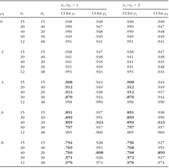
In non-experimental designs wherepis known, stratified random sampling can be used to obtained the desired sample sizes in each group. Researchers often want equal sample sizes to maximize the power of the independent-samplest-test or to minimize the negative effects of assumption violations (Scheffe, 1959). A second Monte Carlo study examined the performance of the confidence intervals forq1andq3with stratified random sampling from a population withp=.20. The results are summarized in Table 7. Unless the fixed sample sizes are selected such thatn1/(n1+n2) =p, the coverage probability of a
95% confidence interval forq1can be far below .95. Poor performance was observed
whenq1= .8. But withp = .20, aq1value of .8 corresponds to ad1value of about 3.33,
which rarely would be observed in any actual study. In non-experimental designs where the minority subpopulation is oversampled in an effort to obtain similar sample sizes, the classical point-biserial correlation should not be used and q3 is the recommended
alternative.
The small-sample coverage probabilities of 95% confidence intervals forq2 andq4
(which are appropriate for experimental designs) were estimated from 100,000 Monte Carlo trials for fixed sample sizes, within-condition normality, homoscedasticity, and heteroscedasticity (r1/r2= 2). The results are summarized in Table 8. With homoscedas-ticity,q2= q4, but with heteroscedasticity ^q2is not a consistent estimator ofq4if the sample sizes are unequal. The confidence interval forq2has coverage probabilities that were close to .95 in the equal sample size conditions under both homoscedasticity and heteroscedasticity. In the heteroscedastic cases with unequal sample sizes, the confidence interval for q2 is liberal when the group with the larger variance has the
smaller sample size and is conservative when the group with the larger variance has the larger sample size. The confidence interval forq2is liberal with moderate and large values
of q2, heteroscedasticity, and equal sample sizes. The confidence interval for q4 has
coverage probabilities that are close to .95 under all conditions.
Confidence intervals for standardized mean differences are not robust to violations of the normality assumption (Bonett, 2009). The coverage probability for a standardized mean difference tends to be conservative with platykurtic (short-tailed) distributions and anti-conservative with leptokurtic (long-(short-tailed) distributions within each level of X. Confidence intervals for point-biserial correlations will have similar properties. The coverage probabilities of 95% confidence intervals for q1
under non-normality and homoscedasticity assuming a simple random sample of size
n= 60 were estimated from 100,000 Monte Carlo trials using four different beta distributions. The results are summarized in Table 9. The beta distribution family has a finite range and is a useful representation of the distribution of the numerous finite-range tests and questionnaires used in psychology. The Beta(1, 1) and Beta(2, 2) distributions are symmetric and platykurtic with kurtosis coefficients of 1.8 and 2.14, respectively. The Beta(2, 4) and Beta(1, 5) distributions are skewed with skewness coefficients of 0.47 and 1.18, respectively, and with kurtosis coefficients of 2.62 and 4.2, respectively. The coverage probabilities of 95% confidence intervals for
q2under non-normality and homoscedasticity with fixed sample sizes were estimated
from 100,000 Monte Carlo trials using the four different beta distributions described above. The results are summarized in Table 10.
The confidence intervalsqjare robust to non-normality with small values ofqj. With
large values of qj, the coverage probabilities can be unacceptably conservative with
transformation is often useful in reducing kurtosis in skewed and leptokurtic distribu-tions. For example, taking the square root of Beta(1, 5) scores produced 95% coverage probabilities closer to .95 for all values ofqj. Although a confidence interval forl1–l2
could be difficult to interpret with transformed data, data transformations do not introduce interpretation problems for the point-biserial correlation because it is a unitless measure of effect size.
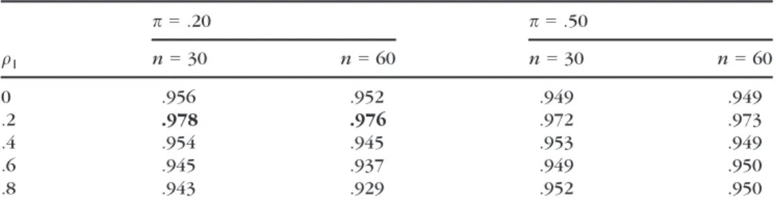
The traditional method of constructing a confidence interval for g2 uses a transfor-mation of a computationally intensive confidence interval for an F non-centrality parameter (Steiger, 2004). The proposed confidence intervals forg2based on confidence intervals forq2
1andq 2
2were examined using 100,000 Monte Carlo trials for random sample sizes (Table 11), fixed sample sizes (Table 12), normality, and homoscedasticity. The coverage probabilities of the 95% confidence intervals were close to .95 for all conditions except forqj = .2, where the coverage probability was closer to .975.
Table 7. Estimated coverage probabilities forq1andq3with normality, fixed sample sizes, andp=.2
q3 n1 n2
r1=r2=1 r1=r2=2
CI forq1 CI forq3 CI forq1 CI forq3
0 15 15 .948 .948 .948 .948 20 40 .950 .947 .950 .947 40 20 .950 .948 .950 .948 30 30 .949 .949 .949 .949 12 48 .951 .941 .951 .941 .2 15 15 .938 .947 .938 .947 20 40 .941 .948 .941 .948 40 20 .941 .945 .941 .945 30 30 .931 .949 .931 .948 12 48 .953 .943 .953 .943 .4 15 15 .908 .944 .908 .944 20 40 .912 .949 .912 .949 40 20 .913 .938 .912 .937 30 30 .870 .944 .870 .944 12 48 .958 .950 .958 .950 .6 15 15 .851 .937 .851 .938 20 40 .859 .951 .859 .950 40 20 .859 .923 .859 .923 30 30 .757 .937 .757 .937 12 48 .965 .960 .965 .960 .8 15 15 .754 .928 .756 .927 20 40 .769 .953 .768 .953 40 20 .769 .898 .768 .899 30 30 .571 .926 .572 .927 12 48 .976 .974 .976 .974
Note. ^q1is not a consistent estimator ofq3unlessn1/(n1+n2)=p. Estimates in each row are based
on 100,000 Monte Carlo trials using randomly generated normal scores within each group. Coverage probabilities less than .925 or greater than .975 are in bold type.
The performance of the varying-coefficient confidence interval was compared with the constant-coefficient and random-coefficient methods form = 5. The formulas given in Borenstein et al. (2009) were used to compute the constant-coefficient and random-coefficient confidence intervals. Four different patterns ofq2were used in the computer simulations comparing the varying-coefficient and constant-coefficient confidence intervals. For each pattern, the varying-coefficient and constant-coefficient point estimates and confidence intervals were computed in 100,000 Monte Carlo trials. Within each trial, scores were randomly generated from a normal distribution with equal variances within and across them = 5 studies. Table 13 compares the performance of the constant-coefficient confidence interval with the varying-coefficient confidence interval for fixed sample sizes ofn1= 20,n2= 30,n3 = 40,n4 = 50,n5 = 60, wherenjis the
sample size per group within each of the m =5 studies. The first row of Table 13 summarizes the performance of the two methods for equal values ofq2across studies and
thus satisfies a primary assumption of the constant,coefficient method. With effect-size equality, both the varying-coefficient and constant-coefficient methods yield nearly unbiased estimates of the average point-biserial correlation and both methods have 95% coverage probabilities that are close to .95. However, with effect-size heterogeneity,
Table 8. Estimated coverage probabilities forq4with normality and fixed sample sizes
q4 n1 n2
r1=r2=1 r1=r2=2
CI forq2 CI forq4 CI forq2 CI forq4
0 15 15 .948 .955 .955 .955 20 40 .950 .952 .887 .951 40 20 .950 .952 .982 .954 30 30 .949 .953 .947 .952 .2 15 15 .948 .956 .944 .954 20 40 .950 .951 .887 .951 40 20 .950 .951 .981 .954 30 30 .949 .953 .947 .952 .4 15 15 .949 .957 .943 .954 20 40 .951 .952 .877 .951 40 20 .951 .952 .974 .953 30 30 .949 .953 .945 .952 .6 15 15 .950 .958 .940 .954 20 40 .953 .953 .861 .949 40 20 .950 .953 .960 .953 30 30 .950 .954 .940 .952 .8 15 15 .951 .958 .932 .952 20 40 .957 .953 .833 .949 40 20 .957 .953 .919 .952 30 30 .950 .954 .931 .951
Note. q1¼q4withr1=r2 =1.^q2is not a consistent estimator ofq4withr1=r26¼1 and unequal fixed sample sizes. Estimates in each row are based on 100,000 Monte Carlo trials using randomly generated normal scores within each group. Coverage probabilities less than .925 or greater than .975 are in bold type.
which is the rule rather than the exception in practice, the varying-coefficient method continues to perform properly, while the performance of the constant-coefficient method is unacceptable with 95% coverage probabilities that are substantially<.95.
The serious limitations of the constant-coefficient meta-analysis methods are now well known (Schmidt & Hunter, 2015, p.368). Bonett (2008a) derived an expression for the large-sample bias of the constant-coefficient point estimator which shows that this estimator is consistent with effect-size homogeneity or with equal weights. In practice, the weights that are used in a constant-coefficient meta-analysis will be unequal and the coverage probability of a 95% constant-coefficient confidence interval can be far less than .95, as illustrated in Table 13.
Random-coefficient methods, which do not assume effect-size homogeneity, have been proposed as a preferred alternative to constant-coefficient methods. Table 14
Table 9. Estimated coverage probabilities forq1andq3with non-normality, homoscedasticity, and random sample sizes (n=60)
Distribution qi
p =.20 p=.50
CI forq1 CI forq3 CI forq1 CI forq3
Beta(1, 1) 0 .952 .936 .949 .948 .2 .951 .940 .950 .949 .4 .950 .951 .955 .954 .6 .949 .962 .963 .963 .8 .952 .990 .979 .979 Beta(2, 2) 0 .952 .937 .949 .953 .2 .951 .940 .950 .953 .4 .949 .950 .953 .957 .6 .946 .966 .960 .963 .8 .945 .986 .972 .974 Beta(2, 4) 0 .952 .936 .949 .948 .2 .951 .941 .949 .949 .4 .947 .951 .951 .951 .6 .941 .965 .955 .954 .8 .936 .981 .960 .960 Beta(1, 5) 0 .953 .928 .950 .949 .2 .949 .935 .948 .948 .4 .940 .943 .942 .942 .6 .924 .952 .934 .934 .8 .904 .955 .917 .917 ffiffiffiffiffiffiffiffiffiffiffiffiffiffiffiffiffiffiffiffi Beta 1ð ;5Þ p 0 .952 .936 .949 .949 .2 .950 .941 .949 .949 .4 .948 .951 .951 .951 .6 .943 .965 .956 .956 .8 .939 .982 .964 .964
Note. Estimates in each row are based on 100,000 Monte Carlo trials using randomly generated Beta (a,b) scores within each group. Coverage probabilities less than .925 or greater than .975 are in bold type. The random sample sizes (n1andn2) were constrained to be>2.
summarizes the performance of the varying-coefficient and random-coefficient methods under some conditions that are nearly ideal for the random-coefficient methods. Within each of the 100,000 Monte Carlo trials, theq2values were randomly selected from a beta
distribution of q2 values, the sample sizes were randomly generated to minimize the
correlation between the Fisher-transformed estimates and the weights, and they-scores within each group were randomly generated from a normal distribution with equal variances within and across studies. The Beta(2, 2), Beta(3, 3), and Beta(4, 4) distributions are symmetric and unimodal. The Beta(3,3) and Beta(4, 4) distributions are also bell-shaped. The results in Table 14 show that the random-coefficient estimator of the average point-biserial correlation is biased and the 95% random-coefficient confidence interval has a coverage probability that is substantially less than .95. In contrast, the varying-coefficient estimator of the average point-biserial correlation is nearly unbiased and the 95%
varying-Table 10.Estimated coverage probabilities forq2andq4with non-normality, homoscedasticity, and fixed sample sizes
Distribution qi
nj=15 nj=30
CI forq2 CI forq4 CI forq2 CI forq4
Beta(1, 1) 0 .947 .955 .949 .952 .2 .949 .956 .950 .950 .4 .954 .961 .955 .958 .6 .962 .968 .964 .967 .8 .978 .982 .979 .981 Beta(2, 2) 0 .947 .955 .949 .953 .2 .949 .957 .950 .953 .4 .952 .959 .953 .957 .6 .959 .965 .960 .963 .8 .971 .975 .972 .974 Beta(2, 4) 0 .948 .955 .949 .952 .2 .949 .957 .950 .953 .4 .951 .958 .951 .955 .6 .954 .961 .954 .958 .8 .959 .966 .960 .963 Beta(1, 5) 0 .949 .958 .949 .953 .2 .948 .957 .948 .953 .4 .943 .953 .943 .948 .6 .933 .945 .934 .940 .8 .916 .929 .915 .923 ffiffiffiffiffiffiffiffiffiffiffiffiffiffiffiffiffiffiffiffi Beta 1ð ;5Þ p 0 .948 .955 .948 .953 .2 .948 .956 .950 .953 .4 .951 .958 .952 .955 .6 .955 .962 .956 .959 .8 .964 .969 .964 .966
Note. Estimates in each row are based on 100,000 Monte Carlo trials using randomly generated Beta (a,b) scores within each group. Coverage probabilities less than .925 or greater than .975 are in bold type.
coefficient confidence interval has coverage probabilities close to .95 under all conditions. Note that the greater bias in the random-coefficient estimator is due primarily to reverse-transforming an average of Fisher-transformed correlations with greater superpopulation heterogeneity.
When using a random-coefficient method, it is important to also report a confidence interval for the variance of the random effect. However, the currently available confidence intervals for the random-effect variance are hypersensitive to minor violations of the
Table 11. Estimated coverage probabilities forq2
1with normality, homoscedasticity, and random
sample sizes q1 p=.20 p=.50 n=30 n=60 n=30 n=60 0 .956 .952 .949 .949 .2 .978 .976 .972 .973 .4 .954 .945 .953 .949 .6 .945 .937 .949 .950 .8 .943 .929 .952 .950
Note. Estimates in each row are based on 100,000 Monte Carlo trials using randomly generated normal scores within each group. The random sample sizes (n1andn2) were constrained to be
greater than 2. Coverage probabilities greater than .975 are in bold type. Table 12. Estimated coverage probabilities forq2
2 with normality, homoscedasticity, and fixed
sample sizes q2 n1=15,n2=15 n1=20,n2=40 n1=30,n2 =30 0 .948 .949 .949 .2 .973 .975 .974 .4 .951 .951 .949 .6 .949 .953 .949 .8 .951 .957 .950
Note. Estimates in each row are based on 100,000 Monte Carlo trials using randomly generated normal scores within each group.
Table 13. Comparison of constant-coefficient (CC) and varying-coefficient (VC) methods forq2
with normality and homoscedasticity
q2 q VC method CC method Average estimate 95% coverage probability Average estimate 95% coverage probability [.3 .3 .3 .3 .3] .3 .298 .947 .303 .944 [.1 .2 .3 .4 .5] .3 .298 .946 .364 .662 [.5 .4 .3 .2 .1] .3 .298 .949 .264 .869 [.5 .2 .1 .2 .5] .3 .298 .948 .322 .904
Note. Estimates in each row are based on 100,000 Monte Carlo trials using randomly generated normal scores within each group. The sample sizes per group were fixed atn1=20,n2=30,n3=40,n4 =50,n5=60 within each trial. Coverage probabilities less than .925 are in bold type.
superpopulation normality assumption, and a very large number of studies are required to assess this critical assumption. A large number of studies are also needed to obtain a usefully narrow confidence interval for the random-effect variance. In contrast, pairwise comparisons or subgroup analyses can be used to effectively describe the nature of effect-size heterogeneity with varying-coefficient methods.
10. Hypothesis tests
10.1. Directional two-sided hypothesis test
In some applications, the researcher simply needs to decide ifqiis either greater than or less than some researcher-specified value (h). The sign ofhwill depend on howX is coded. Ifqiis determined to be>h, this could provide support for one theory or one
course of action, and ifqiis determined to be<h, then this could provide support for
another theory or another course of action. This type of decision for a given value ofais called a directional two-sided test (see Jones & Tukey, 2000). It can be shown that the probability of making a directional error (i.e., deciding thatqi > hwhenqi <hor deciding
thatqi < hwhenqi > h) is at mosta/2, assuming all assumptions of the test have been
satisfied.
A confidence interval forqican be used to conduct a directional two-sided test for the
population point-biserial correlation. Specifically, if the lower limit of the 100(1– a)% confidence interval is>h, then the null hypothesis (qi = h) is rejected and we accept qi > h; if the upper limit of the 100(1–a)% confidence interval is less thanh, then the null
hypothesis is rejected and we accept qi < h; if the 100(1 – a)% confidence interval
includesh, the results are inconclusive.
For the special case ofh= 0, the independent-samplest-test can be used to conduct a directional two-sided test for a population point-biserial correlation. Specifically, if thep -value is<aand thet-value is positive then acceptqi> h; if thep-value is<aand thet-value
is negative then acceptqi < h. If thep-value is>a, the results are inconclusive. Forh= 0,
the independent-samplest-test can be used for all four of the point-biserial correlations becausel1= l2impliesqi = 0 (i= 1,. . ., 4).
A confidence interval forqi1–qi2can be used to conduct a directional two-sided test for
a difference in two population point-biserial correlations that have been estimated from two independent samples. Specifically, if the lower limit of the 100(1–a)% confidence
Table 14.Comparison of varying-coefficient (VC) and random-coefficient (RC) methods forq2with normality and homoscedasticity
Distribution ofq2 q VC method RC method Average estimate 95% coverage probability Average estimate 95% coverage probability Beta(4, 4)–.2 .3 .298 .947 .317 .882 Beta(3, 3)–.2 .3 .298 .947 .322 .856 Beta(2, 2)–.2 .3 .298 .947 .331 .800 Beta(2, 4.65) .3 .299 .948 .322 .862
Note. Estimates in each row are based on 100,000 Monte Carlo trials using randomly generated normal scores within each group. The equal sample size per group for each study was randomly generated from a Uniform(20, 60) distribution within each trial. Coverage probabilities less than .925 are in bold type.
interval is>h, the null hypothesis (qi1–qi2= h) is rejected and we acceptqi1–qi2> h; if
the upper limit of the 100(1–a)% confidence interval is less thanh, the null hypothesis is rejected and we acceptqi1–qi2< h; if the 100(1–a)% confidence interval includesh, the
results are inconclusive.
10.2. Equivalence test
In some two-group studies, the researcher wants to show that two different treatments (e.g., an inexpensive new treatment and the current treatment) or two different demographic subpopulations (e.g., men and women) have similar population means (Wellek, 2010). Suppose two treatments or two subpopulations are considered to be equivalent ifl1–l2is within the htohrange, which is called the range of practical
equivalence (ROPE). A confidence interval forl1–l2can be used to decide ifl1–l2is
inside or outside the ROPE. In applications where the response variable has an arbitrary metric or if the values of the response variable do not have clear clinical interpretations, it could be difficult for the researcher to specify a ROPE forl1–l2. In these situations, it
might be easier for the researcher to specify a ROPE forqi. For example, a researcher might
argue that a point-biserial correlation within the range .1 to .1 represents a small or unimportant difference in population means. A 100(1–2a)% confidence interval forqi
can be used to decide ifqiis within the range htoh, or ifqiis outside this ROPE (Wellek,
2010). If the confidence interval forqiis completely within the ROPE, the two treatments
or subpopulations are declared to be equivalent; if the confidence interval for qi is
completely outside the ROPE, the two treatments or subpopulations are declared to be non-equivalent; and if the confidence interval includes the value horh, the results are inconclusive.
10.3. Non-inferiority test
A 100(1 – a)% confidence interval forqi can be used to conduct a non-inferiority test
(Wellek, 2010). Suppose the ROPE is htohand the goal of the study is to determine if
qi > h(non-inferiority) orqi < –h(inferiority). For this test, acceptqi > hif the lower
limit forqiis greater than–h, and acceptqi < –hif the upper limit forqiis less than–h. The
results are inconclusive if the confidence interval includes the value–horh.In some applications, it is sufficient to show that an inexpensive treatment is not inferior to a more expensive treatment. The traditional t-test of equal population means is not an appropriate test for non-inferiority.
10.4. Directional non-equivalence test
A 100(1 –a)% confidence interval forqi can be used to conduct other non-traditional
hypothesis tests. For example, suppose the ROPE is–htohand the goal of the study is to determine ifqi > horqi<–h. For this test, acceptqi > hif the lower limit forqiis
greater than h, accept qi < –hif the upper limit forqi is less than –h, and accept the
hypothesis of equivalence if the confidence interval for qiis completely within the–h
tohrange. The results are inconclusive if the confidence interval includes the value–h
or h. Compared to the traditional test of qi = 0, where a rejection of the null
hypothesis does not preclude the possibility thatqiis very close to 0, the acceptance of qi> horqi < –hindicates that the value ofqiis at least meaningfully large in addition
11. Sample size planning
11.1. Sample size for desired power
The point-biserial correlations presented here are useful supplements to the independent-samplest-test. When planning a two-group experiment withn2/n1 =rand approximately
equal variances, the values ofn1andn2required for an independent-samplest-test with
power 1–band a Type I error rate ofaare very accurately approximated by the formula
n1¼~r2ð1þ1=rÞðza=2þzbÞ2=ð~l1l~2Þ 2þ
za2=2=4; ð34Þ andn2 = rn1, wherer~2is a planning value of the average within-group variance,l~1~l2is a planning value of the expected difference in population means,za=2 is a two-tailed criticalz-value,zbis a one-tailed criticalz-value, and the adjustmentza2=2=4 is based on results given by Guenther (1981).
Researchers might have difficulty using equation (34) if they have difficulty specifying
~
r2 or the value of~l
1l~2. Given the relation between a point-biserial correlation and standardized mean difference, equation (34) can be expressed as
n1¼ 1~q2 ð Þð1þrÞ 4r h i za=2þzb 2 ~ q2 þz 2 a=2=4 ð35Þ
whereq~is a planning value ofq2. A planning value ofq2could be obtained from expert
opinion, a pilot study, or a review of the literature. Some researchers will find equation (35) easier to implement than equation (34). As can be seen from equation (35), a smaller value of q~ produces a larger sample size requirement. The R function
size.test.pbcor2(Appendix) computes equation (35).
Equations (34) and (35) are appropriate for experimental designs. In a non-experimental design with simple random sampling, the total sample size (n= n1+n2) required to conduct a directional two-sided test of H0:q1= 0 with power 1–band a Type I
error rateais approximately
n¼ 11:5q~2þ ~q2 4~pð1~pÞ za=2þzb 2 ~ q2 ; ð36Þ
where ~p is a planning value of p and ~q2 = ln[(1 + q~)/(1–q~)]/2. The R function
size.test.pbcor1(Appendix) computes equation (36).
11.2. Sample size for desired precision
The hypothesis testing result of an independent-samples t-test does not provide effect-size information. A confidence interval for a population point-biserial correla-tion will provide useful informacorrela-tion about the magnitude of the effect if the confidence interval is sufficiently narrow. When planning a two-group experiment with n2/n1= r and approximately equal variances, the values of n1 and n2 required
to obtain a 100(1 – a)% confidence interval forq2 that has a desired width of about w are approximately
n1¼ 1þr r ~ q2 2 1ð q~2Þþ1 ~ q2 1~q2þ1 3 za=2 w 2 ð37Þ andn2 = rn1. The R functionsize.ci.pbcor2(Appendix) computes equation (37).
When planning a non-experimental study with simple random sampling, the total sample size required to obtain a 100(1–a)% confidence interval forq1that has a desired
width of aboutwis approximately
n¼ 4 1 ~q22 11:5q~2þ ~q 2 4p~ð1p~Þ za=2 w 2 ; ð38Þ
where p~ is a planning value of p. The R function size.ci.pbcor1 (Appendix) computes equation (38).
12. Examples
12.1. Example 1
Howell (2007, p. 200) described a two-group experiment to assess the effect of stereotype threat on mathematics examination performance of college students. The estimated means were 9.64 and 6.58, the estimated standard deviations were 3.17 and 3.03, and the sample sizes were 11 and 12 for the control and stereotype threat groups, respectively. Howell computed a pooled-variance independent-samplest-test and obtainedt(21)= 2.37,
p=.027. This result allows us to reject the null hypothesis of equal population means at
a=.05 and conclude that the population mean in the control condition is greater than the population mean in the stereotype threat condition.
To describe the magnitude of the population effect size, a confidence interval forl1– l2, a standardized mean difference, or a point-biserial correlation should be reported along with thet-test result. The sample sizes are too small to assess homoscedasticity, and it is prudent to report a 95% confidence interval forq4rather thanq2. Using the R function
ci.pbcor124 (Appendix), the point estimate of q4 is .446 and the 95% confidence interval forq4is [.037, .689]. It could be argued that this confidence interval is too wide to provide useful scientific or practical information and the study should be replicated using a larger sample size. Using the R functionsize.ci.pbcor2(Appendix) witha = .05, a point-biserial planning value of .446, assuming equal sample sizes per group, and a desired 95% confidence interval width of .3, the required sample size per group in a replication study is about 50.
The sample size required to achieve desired precision is often substantially larger than the sample size required to achieve desired power of a two-sided directional test. Using the R functionsize.test.pbcor2(Appendix), the sample size required to conduct an independent-samplest-test witha = .05, power of .9, and a point-biserial effect size of .446 is about 23 per group.
12.2. Example 2
Wright, Quick, Hannah, and Hargrove (2017) developed a new scale to measure ‘character’ in which one of the subscales was a measure of ‘valour’. One of the goals of this study was to develop a new measure of valour that is not gender-biased (T. A. Wright, personal communication). They conducted two studies. In one study they obtained a
simple random sample of college students, and in a second study they obtained a simple random sample of working adults. The members of each sample were classified into male and female groups. Using the reported descriptive statistics in Wrightet al.(2017) and utilizing the R functionci.pbcor124(Appendix), the estimate ofq1is .052 with a 95% confidence interval of [–.053, .156] for the college students and –.068 with a 95% confidence interval of [–.187, .053] for the working adults. Using the R function
ci.diff.pbcor(Appendix), a 95% confidence for the difference inq1values in the two populations is [–.040, .278]. This confidence interval includes 0, which could justify an examination of the average point-biserial correlation in the two populations. Using the R functionci.ave.pbcor(Appendix), an estimate of the average of theq1values in the
two populations is–.008 with a 95% confidence interval of [–.088, .071]. Note that the confidence interval for the average point-biserial correlation is substantially narrower than the confidence interval for each separate population and narrow enough to perform an equivalence test. If we assume that a point-biserial correlation between valour and gender of less than about .1 is evidence of gender equivalence, then the confidence interval for the average point-biserial correlation suggests that the gender bias in the new valour scale is small and unimportant.
13. Conclusion
Each point-biserial correlation is appropriate in specific types of applications. The classical point-biserial correlation (q1) is appropriate in both experimental and
non-experimental designs if the homoscedasticity assumption can be justified. The classical point-biserial correlation also is appropriate in non-experimental designs with heteroscedasticity if simple random sampling is used. Theq2measure of point-biserial correlation is appropriate in experimental designs with equal or unequal sample sizes if the homoscedasticity assumption can be justified. The q3 measure of point-biserial correlation is appropriate in non-experimental designs with stratified random sampling, equal or unequal sample sizes, and heteroscedasticity. Theq4measure of point-biserial correlation is appropriate in experimental designs with equal or unequal sample sizes and heteroscedasticity. The appropriate types of applications for the four point-biserial correlations are summarized in Table 15.
The current practice of reporting thep-value for an independent-samplest-test along with only a sample value of a standardized mean difference or a point-biserial correlation
Table 15.Summary of point-biserial formulas and applications
Parameter Point estimator equation Confidence interval equations Applications
q1 (12) (25) and (26) Experimental or non-experimental designs with equal or unequalnjand equalr2j; or non-experimental designs with unequalr2
j and simple random sampling
q2 (14) (25) and (28) Experimental designs with equal or unequal
njand equalr2j
q3 (15) (25) and (27) Non-experimental designs with stratified random sampling, equal or unequalnjand equal or unequalr2j
q4 (16) (25) and (28) Experimental designs with equal or unequalnjand equal or unequalr2
can be more misleading than reporting only thep-value. In Example 1, the sample point-biserial correlation was .442 (which could interpreted as a ‘large’ effect), and it would be tempting to conclude that stereotype threat had not only a statistically significant effect but also a large effect on performance. However, the 95% confidence interval [.039, .687] for the population point-biserial correlation provides important additional information and suggests that the population point-biserial correlation could be trivial or very large. In this case, a larger sample is needed to more accurately assess the size of the stereotype threat effect. The confidence intervals for point-biserial correlations presented here can be used to supplement the results of an independent-samplest-test with useful effect-size information.
In studies with two independent samples, the t-test for equal population means is typically performed, but several non-traditional hypothesis tests (e.g., equivalence test, inferiority test, directional equivalence test) can also be performed. These non-traditional tests require the researcher to specify a ROPE, but this might be difficult to do in terms of a mean difference. When the effect size is expressed as a point-biserial correlation, it is usually easier to specify a ROPE. The confidence intervals for a population point-biserial correlation presented here can be used to perform a variety of useful non-traditional hypotheses tests.
The point-biserial correlation is a commonly used measure of effect size in meta-analyses. The currently used constant-coefficient and random-coefficient meta-analysis methods for point-biserial correlations have serious limitations, and their continued use is difficult to justify. The varying-coefficient meta-analysis methods for point-biserial correlation presented here have excellent performance characteristics and do not make any of the unrealistic assumptions of the constant-coefficient and random-coefficient methods. With the new point-biserial correlations introduced here, the most appropriate type of point-biserial correlation can be computed for each study and then combined in the meta-analysis.
In a study that has used a sample size that is too small, hypothesis tests will have low power and confidence intervals could be uselessly wide. Sample size planning is perhaps one of the most important steps in the design of a proposed study. The sample size formulas presented here can be used to design a study that will have an acceptably narrow point-biserial confidence interval or a hypothesis test with desired power.
References
American Psychological Association (2010).Publication manual of the American Psychological Association(5th ed.). Washington, DC: Author.
Arnold, S. F. (1990).Mathematical statistics. Englewood Cliff, NJ: Prentice-Hall.
Bonett, D. G. (2008a). Confidence intervals for standardized linear contrasts of means.
Psychological Methods,13, 99–109. https://doi.org/10.1037/1082-989X.13.2.99
Bonett, D. G. (2008b). Meta-analytic interval estimation for bivariate correlations.Psychological Methods,13(3), 173–181. https://doi.org/10.1037/a0012868
Bonett, D. G. (2009). Estimating standardized linear contrasts of means with desired precision.
Psychological Methods,14, 1–5. https://doi.org/10.1037/a0014270
Bonett, D. G., & Price, R. M. (2015). Varying coefficient meta-analysis methods for odds ratios and risk ratios.Psychological Methods,20, 394–406. https://doi.org/10.1037/met0000032
Bonett, D. G., & Wright, T. A. (2007). Comments and recommendations regarding the hypothesis testing controversy.Journal of Organizational Behavior,28, 647–659. org/10.1002/job.448