A New Energy-efficient Multi-target Coverage Control Protocol Using Event-driven-mechanism in Wireless Sensor Networks

A New Energy-efficient Multi-target Coverage Control

Protocol Using Event-driven-mechanism in Wireless

Sensor Networks

https://doi.org/10.3991/ijoe.v13i02.6465

Zeyu Sun

Luoyang Institute of Science and Technology, Luoyang, China Xi’an Jiaotong University, Xi’an, China

[email protected]

Rong Tao*

Luoyang Institute of Science and Technology, Luoyang, China [email protected]

Longxing Li

Luoyang Institute of Science and Technology, Luoyang, China [email protected]

Xiaofei Xing

Guangzhou University, Guangzhou, China [email protected]

Abstract—The covering problem and node deployment is a fundamental problem in the research into wireless sensor networks. The number of nodes and the coverage of a network can directly affect performance and operating costs. For this reason, we propose Event-driven-mechanism Coverage Control Protocol (ECCP). The algorithm uses the correlation between the nodes and dy-namic grouping to adjust the coverage area. Within the coverage area, we use the greedy algorithm to optimize the coverage area. So the target node is uni-formly covered by other sensor nodes and the network resource is optimized. To ensure the energy balance in the wireless sensor network and extend its life-time, we only wake partial nodes to work in a cycle, so that they can work in turn. Experiments show that the algorithm can effectively reduce energy con-sumption, with better adaptability and effectiveness.

Key Words—wireless sensor networks, energy efficient, coverage control pro-tocol, network lifetime

1

Introduction

widely used in national defense, transportation, medical, environment monitoring and various scientific fields [1-2]. Coverage is the fundamental issues in a WSN. Node deployment and plan can effectively reflect the monitor of physical space and directly affect the service quality provided by the network. Through the node relevance and dynamic adjustment to improve network coverage, and improve its ability to imple-ment target monitoring, data obtaining and data processing tasks are utilized with the help of a greedy algorithm to optimize network resource allocation [3-4]. In addition, how to optimize the node configuration with minimal working nodes for effective monitoring and covering and low energy consumption while satisfying the coverage quality is a key problem in WSN. In recent years, numerous scholars and experts have carried out much effective research about the coverage and energy consumption of WSN, and have made some progress. An efficient bipopulation-based evolutionary full area coverage (BEFAC) algorithm is proposed here. The algorithm constructs a complete coverage area mainly based on population optimization, and through the adaptive function to calculate the minimum number of required nodes within the monitoring area, finally determines the minimum number of nodes and the corre-sponding coverage.

A centralized k-degree coverage protocol is given in paper [5]. The network model is established mainly through the communication function between nodes and the node perception area in this protocol, and uses a proportional relationship between the models to determine the k-degree coverage.

Paper [6] introduces an energy-saving coverage calculation method. This method obtains the coverage of the target node through the way node moves. In the direction of energy, it achieves effective coverage of the monitoring area by the scheduling policy of nodes.

Paper [7] proposes a linear energy-saving coverage method, by scheduling the nodes and supplying them after the completion of certain coverage to extend the life-time of the network.

The constraints of the algorithms above are based on a perceptual model. Using the geometric calculation method allows redundant nodes dormancy by a scheduling mechanism. But in the actual application, it is often restricted by external factors. In the theoretical calculation, the network model is too idealistic with a high complexity. We present here an energy efficient multi-target associated coverage algorithm. Cov-erage is over the monitored area as long as it meets certain covCov-erage criteria from the perspective of the coverage accuracy. Let some nodes be in a working state by using the sensor scheduling strategy in the covering process, and the remaining should be in a dormant or other state. Then optimize by a greedy algorithm and wake some nodes after a period of !i. Then, regroup the target and nodes and repeat the above until the

2

Network model and analysis

2.1 Problem description

This research is based on the following basic assumptions:

Assumption 1: the communication range and sensing range of the wireless sensor networks are disc-shaped.

Assumption 2: coverage radius of nodes is equal, and the movement of nodes is synchronized and parallel.

Assumption 3: the node localization is acquired by a position algorithm.

According to the situation, in order to obtain data exactly and comprehensively, a large number of sensor nodes should be deployed in the monitoring area to multiple-cover the target [8-9]. However, the conclusion is opposite from the perspective of energy consumption. So it is better to multiple-cover the target node only and allow the others to remain.

Definition 1: Suppose a given target node set is T={t1,t2,t3…tk},and the sensor node

collection is V={v1,v2, v3…vn}. At a certain point, if an arbitrary target node tk from set T is covered by at least one node form collection V , then the target set T is fully cov-ered.

Definition 2: Assuming sensor nodes Si and Sj, which are responsible for

monitor-ing region Ci and Cj that Ci!Cj!", therefore sensor nodes Si and Sj exist in a

relation-ship called covering association. Let t be a set of m target nodes randomly surrounding the monitoring area, and K is the edge set of the network graph which represents eij=1

among all eij. eij means the position relationship between sensor node Si and target node Tj. When ei=1, if and only if the Euclidean distance between the target Tj and the

sen-sor node Si is less than or equal to the R which is radius of perception of sensor node,

otherwise ei=0. W={w1,w2, w3…wn} is the initial energy set of sensor nodes and it

follows with a normal distribution W~N(u,"2). wi represents the initial energy of sensor

node si. wi is also the maximum number of node energy during operation.

Definition 3: When any target node in the monitoring area is simultaneously covered by k sensor nodes, called k degree coverage, it is also known as c k

k i

i c A +As!

=

"!

which 1#c#n. Generally the attention of a target is directly reflected by the coverage number.

2.2 Solution problem

The case is more suitable for data acquisition operations for wireless sensor networks. The first scenario is adapted to some simple questions, which means that each sensor node in a wireless sensor network should make the point as the center of a sensitive area with a radius r. Each sensor node can collect or retrieve the every target node within the signal field with a certain amount of accuracy.

The second scenario can be applied to some more complex problems. In this paper, we will research a space homologous random field [10-12]. In the first case, all the target nodes (x,y)A, S(A) have a mean value µ subordinate to variance !2. In the

second case, the relationship between any two sensor nodes in set A is determined by the Euclidean distance between two points:

(

) (

)

(

)

(

) (

)

(

)

(

)

(

(

)

)

( )

2 2

1 1 2 2 1 2 1 2

1 1 2 2

, , ,

, ,

R x y x y x x y y

E S x y u S x y u R d

= ! + !

" #

= _$ ! ! _%= (1)

The equation achieves the measured value S(x,y) of the target node (x,y), and completes the collection of data for an access point, which contains some measurement data.

Suppose M represents all nodes which are retrieved for data collection. Mis the complementary set of A. The data obtained from M are used for reestablishing a random field S(A). The sensor node which is closest to the point (x,y) in M is used to calculate a measurement value for estimating the signal field in M. Therefore, the estimated value Se(x0,y0) in (x,y) can be calculated as follows:

Se(x0,y0)=#S(x,y) (2)

(x1,y1)= mind((x0,y0),(u,v)) (3)

where (u,v) is the closest point to (x,y) in M. When meeting the requirements of network service quality, we define the maximum distortion D as follows:

E[(Se(x,y)-S(x,y))2]"D (4)

In considering residual energy and space contact in the signal field, in order to prolong the network lifetime in each data retrieval operations, it is necessary to select a subset from the available sensor nodes for collecting data. Therefore, the subset ensures requirements of a particular network service. So far, the problem addressed in this paper is how to select an optimal subset of sensor nodes in each data collection, which can be used for reestablishing the network and maximize the lifetime of the network.

Definition 4: To an arbitrary mobile node i in the position xi, the exclusive force

between i and any other mobile node j that in position xj is defined as follows:

( )

( )

( )

( )

2

1 1 _,

, ,

0 , i j

exc

x x

k d i j r

r d i j

F d i j

d i j r

! " #" $ #

% & $ '& ' (

% & '& '

= ) * +* +

%

> %,

(5)

In this function, D(i,j) means the Euclidean distance between the sensor node i and the node j. Fexc represents the exclusive force and r is the sensor radius of the sensor

node.

( )

( )

( )

( )

2

1 _{, 2}

, ,

0 , 2

i j

att

x x

k d i j r

d i j

F d i j

d i j r

! " # $

>

% &_& '_'

= ( ) *

% ₊

,

(6)

In order to avoid the attractive and exclusive force being too big or too small, a dimensionless ratio k is introduced so that the range of both forces can be adjusted. Combine the formulation (5) and (6), then:

( )

( )

1

2

, =

,

exc c

j

att c

j

F F i j

F

F F i j

!"

!"

# =

$ %

= $ &

'

'

(7)

In formulation (7), Fc1 represents the exclusive force to node Si, and Fc2 is the

at-tractive force. For the circle of the coverage area, and the target area boundaries of exclusion and attraction of the mobile node can also be applied to other models. In this condition, ximeans the position of the mobile node i to the vertical projection

point of the target area’s boundary which is closest to node i. If the random perturba-tion force between the nodes is also considered, the resultant force of a node can be:

(

1 2 3 4

)

i exc att bor wan

F =

"

!F +!F +!F +! F (8)

Fboris the exclusive force from the edge of the target area to the sensor node, Fwan

on behalf of the mutual perturbation force and set $ be the control parameter of each force. The motion equation of the mobile node i at moment t can be defined as

( )

(

)

'' '

i i

v x = F !µx m where u means a damping coefficient and m is the virtual quality of nodes.

The mobile node is defined by the virtual force and vector relationship [13-14]. The deployment of sensor nodes is random the first time, which means that each sensor node’s position is an arbitrary pattern. Between any two nodes, there exists a virtual force which creates a stable and balanced state for each sensor node, similar to the vertex position of the regular hexagon [15-16]. At the initial moment, the direction of virtual force lies between six nodes which are the vertices of a regular hexagon using S as its central position is transmitted in the form of broadcasting to search its six neighborhoods. Suppose Si is a sensor node inside a regular hexagon which receives

message S from the right lower section and receives S3 message from left lower section.

The Euler equation is used to solve the Euler distance between node S and Si, Dssi ! "!!

is the direction and angle % is the inner product of Dss3

! "!!!

andDssi ! "!!

, that is:

!

=

arccos

D

ss3

! "

!!!

!

D

_ss

i

! "

!!

D

_ss3

! "

!!!

D

_ssi

! "

!!

₍₉₎

(

2 2

)

1₂

3i i 2 i cos

s s ss ss

d = d +r " d r

!

(10)

The same method can be used to solve &. The power and direction of the exclusive force, which is also a vector relationship of Siis obtained by plugging formulas (9)(10)

(

)

2 3 3

2 2

3 3

1 1 1 1 _cos

i i i i

s si s

exc

ss ss s s s s

x x x

F k

r d d r d d ! "

# $# % $ # $# $

= '_' % ('_(' ( '_{( '}& % ('_(' (₍& +

) *) * ) *) *

(11)

The specific process is that the six sensor nodes selected from the sensor node will summarize the sensor node's instructions, turning the original sleep state to an active state. If the six neighbor nodes are independent of each other, then they move to the top of the regular hexagon, forming relatively stable position information and sending this message to S. When the message is received by S, it will remove the sensor node Si inside the hexagon whose Euler distance, which can be determined by formulas (9), (10) and (11), is less than the sensor radius out of the regular hexagon. At the same time, the sensor node S is shut down to reduce energy consumption and improve the entire network life cycle [17].

Theorem 1: Assuming the occurrence probability of the target area covered by the sensor node is p, set k=2 means the target node is multiple covered twice, and let m represent the times of the target node that moves in the first round and n represent times second round. Then the probability of occurrence is p2_qn-2_{, conditional}

possibil-ity is pqn-m-1 _{, where q=1-p}

Proof: Suppose X represents the times of the node that moves the first time and Y means the times second time, in the first round, m is the value of X. In the second round, the target node is precisely covered by the sensor node twice, and n-2times is not covered. So the probability of occurrence is shown as follows:

P(X=m,Y=n)=p2_qn-2 ₍₁₂₎

The joint probability of first and second times is:

(

)

2 2 1

1

n m

n m

P X m ! p q" pq "

= +

= =

#

= (13)

(

)

(

)

2 2 1

1 1

, = n m

n m n m

P X m ! P X m Y n ! p q" pq "

= + = +

= =

#

= =

#

= (14)

According to the multiplication formula of probability:

(

)

(

(

)

)

2 2 1

1

,

= n n m

m

P X m Y n p q

P Y n X m pq

P X m pq

!

! ! !

= =

= = = =

= (15)

3

ECCP algorithm optimal scheduling strategy

3.1 Ant colony optimization and probability evolution

Covering control is always significant for the efficiency of wireless sensor network coverage [18-19]. How to effectively deploy sensor nodes in the monitoring area, reduce the consumption of sensor energy in the process of deployment, extend the life cycle of the entire network, decrease the generation of redundant code and increase the transmission ratio of communication channels are the focuses in the current re-search.

algorithm, the working space is a continuous search space and all sensor nodes are moved to the ideal region through the adaptation function.

The local fast convergence of ACO and the global search feature are integrated with the characteristics of wireless sensor networks, which make the sensor nodes more flexible in the deployment process, reducing the cost of network energy and prolonging the network lifetime.

Definition 6: During the process of traversal searching, ants take advantage of in-formation on each path and heuristic inin-formation of the path to calculate the probabil-ity of state transition. Let the probabilprobabil-ity of transition between any two nodes be p, then:

( )

( )

( )

( )

1

0

ij ij ij ij

s allowed

t t t t s allowed

p

s allowed

! " ! "

# $ # $ % & ' _{( )} * + * + * + * + ,

-_{0 1 0 1. 0 1 0 1/}

=_{2 3 4}

- ₅

6

7

₍₁₆₎

In this formula, ' represents the heuristic information factor which indicates the relative importance of trajectories, reflecting the usage of information accumulated during the movement of ants when ants are moving. With the increment of the value of indicating that the ant is more likely to choose the path on which other ants have passed, then the collaboration between ants becomes tight. & as the expected heuristic

factor represents the relative importance of visibility. It reflects the weight of heuristic information for the ants concerned in the process of path selection. The larger the value of&, the greater is the probability that the state transition is closer to 1, which is the greedy algorithm. !ij(t) and(ij(t) denote the pheromone residue function between

any two paths and the heuristic function respectively. In order to avoid the operation of the heuristic information being too greatly influenced by the residual information, the amount of residual information in the path is updated with each iteration. The updating formula is as follows:

(

) (

) ( )

( )

1

1 1 m k

ij ij ij

k

t t t

! " ! " !

=

+ = # +

%

$ (17)

Where ) range )$[0,1] indicating that the pheromone evaporation coefficient, 1-)

as residual pheromone factor on the path. ( )

1 m k ij k t ! = "

#

, which represents the increment of residual pheromone that former k ants have left.

Theorem 3: In the target area, the coverage ratio of the sensor nodes is p, and the maximum upper limit for the iteration is N. Until the target node is fully covered, the expected value of the sensor nodes is: E(X)=[1-(1-p)N_]p-1

Proof: Let X be the times of the target nodes transferring in the first covering and X%[0,1,2…N]. In the case of x=k and 1#k#N-1which means the former N-1 times do not cover the target node. Therefore, the distribution density function of X is:

(

)

(

)

(

)

1

1

1 =1,2,3 -1

1 =

k

N

p p k N

P X k

p k N

! ! " _! # = =_$ ! #% ! (18)

( )

1

(

)

1

(

)

1

1

1 1

N _{k N}

k

E X !kp p ! N p !

=

Let q=1-p, 1 ( ) 1 1 1 N k k

S !k p !

=

=

"

! , then 1 1

1 N

k k

S !kq!

=

=_" multiply q on both sides of the equation,

that is 1 1 N

k k

qS !kq

=

=_" as:

(

)

1

(

)

2 1 1 1 1 1 1 1 N N

k N N

k

q

q N q N q

q ! ! ! ! = ! ! ! = ! ! !

"

(20)

(

)

(

)

1

(

)

1

(

)(

)

1

1

2 2

1 1 1 1 1

1

1 1

N N

N

N _{N q p N p}

q S

q p p

q ! ! ! ! _{! ! ! ! !} ! = ! = ! ! ! (21)

Put S into formula (22):

( )

(

)

(

)(

)

(

)

(

)

(

)

(

)

1 1 1 2 1 1 1

1 1 1 1

1

1 1 1

= = 1 1

N N

N

N N

N

p N p

E X p N p

p p

p p p

p p p ! ! ! ! ! !

" _{! ! ! !} #

$ % = _$ ! _%+ ! & ' ! ! + ! _{( )} ! ! * + (22)

Corollary 1: When the sensor nodes cover a certain region of the target area, the minimum probability of the entire network working normal is p1 and p2 (p1>p2) is the

coverage rate of the working node. The minimum required number of sensor nodes N is as follows when the coverage ratio of whole network is not less than p3(p3>p2).

N=k2_p

1(1-p1)(p1-p2)-2, where k=*-1(p3)

Proof: According to De Laplace central limit theorem:

(

)

(

)

(

)

(

)

(

)

(

)

1 2 1

2 2

1 1 1 1

1 2 1 2

3

1 1 1 1

1 1

1 1

1 =

1 1

X P N P N P N

P X P N P X P N P

NP P NP P

P N P N P N P N _P

NP P NP P

! !

" _{$ $} #

% &

' = $ < = $ <

% _{$ $} &

( )

" _$ # " _$ #

% & % &

* $ $ '

% _$ & % _$ &

( ) ( )

(23)

Let k=*-1(p3), then equation (24) can be transformed into 1 ₍ 2 ₎

1 1 1

PN P N _k

NP P

! "

! . So the

so-lution of N is:

N=k2_p

1(1-p1)(p1-p2)-2 (24)

Theorem 4: In a monitoring area, when a wireless sensor network consisting of N sensor nodes which has one and only one sensor node is transmitting the package and the probability value of the node is 1/(N+1-i), the value of pi-max will be the maximum.

Proof: In the monitoring area, all sensor nodes are independent with each other. The probability of only one node that is working is represented as#, and when N sen-sor nodes are working at time t0, the coverage probability of a single sensor node is:

(

)

1

1 ₁ N

i N

p C= ! "! " (25)

The probability event meets the geometric distribution of time consumed. So in this monitoring area, when there are N+1-i nodes working together, the probability of a single node successfully covering the region is:

(

₁

)

1

(

₁

)

N 1i 1

(

₁

)

N i

i N i N i

p = "! C "! "! +" =C "! "! " (26)

Doing the derivation on the left side of this equation and making its result 0, then:

(

)

1

(

)

1 ₁ N i _{1 0}

N i

C " "! " "%# " "! N i" !$&= (27)

Discussion: In the first case, by the related knowledge of probability theory, the value of probability is non-negative and no larger than 1, as #%[0,1]. When #=1,

which means the single sensor node can completely cover the monitoring area, this is in conflict with the situation that there exist N+1-i nodes working. #!1. In the case of

#=0, that means no sensor node is working, and this also shows the contradiction, so

#%(0,1). When 1-#-(N-i)#=0, the result of #=1/N+1-i can be solved. piwill be the

maximum value when#=1/N+1-i. Let u=N-i+1 which also means #=1/u, and plugging them into formula (26):

(

1 1

)

1 1

(

₁

)(

₁

)

1 1

1 =

1

u

u u N i

i u

u _{u u}

u N i

u p

u u u N i

!

! +!

" #

! _$ ! _%

! ! " ! # " ! #

& '

= = _{$ %} =_{$ %}

+ !

& ' & ' (28)

That is: 1

_ max ₁

N i

i

N i p

N i

+!

!

" #

=$_{& + !} %_' .

3.2 Dynamic parameter setting and updating strategy

In the covering the optimized process of the wireless sensor network, the final des-tination is determined through the ant colony algorithm (ACO) which involves a mov-ing procedure of rapidly travelmov-ing sensor nodes. There exist various parameters in the ACO, and each parameter has its own practical significance.

Reasonable parameter setting can improve the convergence rate of the system, en-hance the search ability of the overall situation, and effectively inhibit the premature stagnation phenomenon.

In case the value of ' is too large, it will lead to positive feedback on the local

op-timal path and the algorithm is prone to premature convergence. In another case, if the value of ' is small, the speed of convergence is not only slow, but also easy to fall into a local optimal solution. When the value of & is the coverage, it speeds up the convergence rate of the system and makes the system search ability decreased which can easily fall into a local optimal solution. Conversely, the small & makes the

con-vergence speed very slow, and it is hard to find out the optimal solution. The adjust-ment formula of abnormal', & is as follows:

(

)

( )

1 otherwise

ij t ij t

!" # #

" "

+ $

%&

=_'

&( (29)

(

1

)

( )

t

otherwise

ij t ij

!" # #

" "

+ $

%&

='

&( (30)

Where k is the proportional coefficient, k=!ij(t)/!ij(t+1). k can complete the dynamic

ad-justment of ', & ensuring the effectiveness of the algorithm. When the optimal value of the algorithm is not significantly changed in the maximum cycle Nc_max, then the value

( )

(

)

(

)

min min

0.95

1 0.95

1

otherwise

t

t

t

!

!

!

!

!

"

" #

$%

=

&

%'

(31)

In the ant colony algorithm, the ants move to the next position in the unit time, so the pheromone on the path will increase hugely, this makes the majority of ants choose the same path. When ants choosing the same path reach a certain number, the current distance is longer than the previous optimal path length and terminates the traversal, increasing the ant’s selection of other paths, and diversifying the searching solution. The updating strategy of the pheromone is updated according to formula (32).

3.3 ECCP algorithm description

In the need of algorithm description, the target set is expressed as T={t1,t2,t3…tk}

and the sensor node set is indicated as S={s1,s2,s3,…sn}. Because the frequent item is 2,

any target node is covered by two or more sensor nodes.

Step 1: deploying N sensor nodes randomly within the target monitoring area, select the target set from frequent item set Tmax and sensor node set Smaxby the coverage area

and the relationship between the sensor node and the target node, where the high-energy sensor nodes can be selected.

Step 2: Let the optimal subset G’(S’,T’,E’,W’)= G(S,T,E,W), greedy algorithm be applied to calculate the coverage set and energy consumption of a target node. When the energy of a target node is less than a specific value, return to G#. Otherwise, select a higher energy sensor node as a coverage node.

Step 3: After removing the selected frequency items from set T, a new target set T1k

is formed. Determine whether the target set T1k is empty. If empty, go to step 5. Step 4: Apply the greedy algorithm. Suppose input items: G(S,T,E,W); output items: optimal subset SN={Shn|n=1,2,3…}. Initialize SN=", n=1, G’(S’,T’,E’,W’)= G(S,T, E,W),

judge whether SN is empty. If not, SN=SNShnn=n+1.

Step 5: Calculate the energy cn of the converged target area for the current sensor node. If cn$w, go to step 2.

Step 6: Calculate whether a target node exists that is uncovered. If it exists, the target is covered only by one sensor note. If the targets are all covered, then complete coverage is achieved.

4

ECCP algorithm system evaluation

Fig. 1. 100*100m2_{, Number of Nodes and Network Lifetime}

Fig. 2. 100*100m2_{, Number of Target and Network Lifetime}

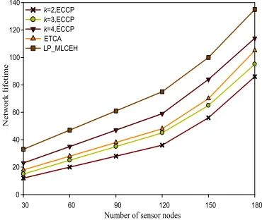
Fig. 3. 200*200m2_{, Number of Nodes and Network Lifetime}

Number of sensor nodes

10 20 30 40 50 60

Network lifetime

0 10 20 30 40 50 60 70 80

k=2,ECCP k=3,ECCP k=4,ECCP ETCA LP_MLCEH

Number of target nodes

5 10 15 20 25

0 20 40 60 80

Network lifetime

k=2,ECCP k=3,ECCP k=4,ECCP ETCA LP_MLCEH

30 60 90 120 150 180 0

20 40 60 80 100 120 140

Number of sensor nodes

Network lifetime

Fig. 4. 200*200m2_{, Number of Target and Network Lifetime}

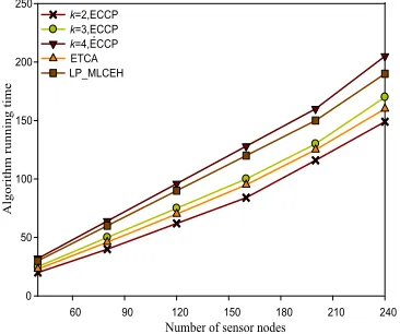
Fig. 5. 300*300m2_{, Number of Nodes and Network Lifetime}

Fig. 6. 300*300m2_{, Number of Target and Network Lifetime}

10 20 30 40 50

0 20 40 60 80 100 120 140

Number of target nodes

Network lifetime

k=2,ECCP

k=3,ECCP

k=4,ECCP ETCA LP_MLCEH

60 90 120 150 180 210 240 0

50 100 150 200 250

Algorithm running time

Number of sensor nodes

k=2,ECCP k=3,ECCP k=4,ECCP ETCA LP_MLCEH

60 90 120 150 180 210 240

0 50 100 150 200 250

Algorithm running time

Number of sensor nodes

k=2,ECCP

k=3,ECCP

From Fig.1 to Fig.3 the network energy consumption is shown in different monitoring areas. Energy-efficient target coverage algorithm (ETCA) [13] and Linear programming maximum lifetime coverage with energy harvesting (LP_MLCEH) [18] are contrasted in algorithms of the proposed algorithm. Figure 3 shows that at the beginning period of three algorithms, the network lifetime was increased with the increase in the number of nodes. However, due to the limit in the range of parameters and the closed state of the redundancy nodes, the network lifetime in our algorithm is less than that of the other two algorithms at the balance of the network energy state. For the same reason, the network energy is also less than that of the other two algorithms in the process of covering the target node. In figure 4, due to the expansion of the monitoring area, most of the redundant nodes are in a working condition, which prolongs the network lifetime. When k=3, the network lifetime. Calculated from the proposed algorithm was greater than that of the ETCA algorithm; when k=4, the network lifetime was greater than that of the contrasting algorithms. From Fig.5 to Fig.7 can be illustrated the changing process of the network lifetime during the process of the coverage of the target nodes. With the increase in the number of target nodes, network lifetimes of the three algorithms were reduced and finally attained a balance. But the average decline rate of our algorithm was less than that of the other two algorithms during the process of decline. The main reason for this phenomenon is when some parts of the monitoring area have dense sensor nodes, which means that the expected coverage value of the area is larger than the others. Wake up partially redundant sensor nodes in working condition by the scheduling mechanism of sensor node, will increase the coverage strength and improve the network lifetime. The same principle described above can be applied to a monitoring area of 300*300m2_.

5

Conclusion

In this paper, we proposed an energy-efficient multi-target association covering algorithm through theoretical analysis of a wireless sensor network. The algorithm makes full use of the association between sensor nodes and target nodes and a wake-up mechanism to achieve the coverage of the target nodes in the monitoring area. In terms of extending the network lifetime, we designed a wireless sensor network lifetime problem to search for the maximization of the coverage set under conditions of constrained energy , and then the greedy algorithm and scheduling mechanism were converted dynamically to resolve this problem. The experimental results show that the proposed algorithm effectively prolongs the wireless sensor network lifetime. In future work, we will focus on how to solve the multi-hop transmission energy consumption problem between sensor nodes and access points, how to realize the random quadratic linear regression and how to improve the quality of unrestricted coverage.

6

Acknowledgment

Educa-tion Department Natural Science FoundaEduca-tion under Grant No.15A413016 and No.17A520044; Cultivation Young Key Teachers in Colleges and Universities of Henan under Grant No.2016GGJS-158; the Guangdong Natural Science Foundation of China under Grant No.2016A030313540, and Guangzhou Education Bureau Sci-ence Foundation under Grant No.1201430560, Shaanxi Education Bureau SciSci-ence Foundation under Grant No.2016SF-428.

7

References

[1]Tseng YC, Chen PY, Chen W. (2012). k-angle object coverage problem in a wireless sen-sor networks. IEEE Sensen-sor Journal, 12:3408-3416 https://doi.org/10.1109/JSEN.2012. 2198054

[2]Habib A, Sajal DK. (2012). Centralized and clustered k-coverage protocols for wireless sensor networks. IEEE Transactions on Computers, 61:118-132 https://doi.org/10.1109/ TC.2011.82

[3]Seok JH, Lee JY, Lee JJ. (2014). A Bipopulation-based evolutionary algorithm for solving full area coverage problems. IEEE Sensor Journal,13:796-807

[4]Mihaela C, JIE W. (2005). Energy-efficient coverage problems in wireless ad-hoc sensor networks. Computer Communications, 29:413-420

[5]Zhao Q, Gurusamy M. (2008). Lifetime maximization for connected target coverage in wireless sensor networks. IEEE/ACM Transactions on Networking,16:1378 -1391 https://doi.org/10.1109/TNET.2007.911432

[6]Jiang HB_{Jin SD Wang CG. (2011). An energy-efficient framework for} clustering-based data collection in wireless sensor network. IEEE Transactions on Parallel and Dis-tributed Systems, 22:1064-1071 https://doi.org/10.1109/TPDS.2010.174

[7]Zhu JM, Hu XD. (2008). Improved algorithm for minimum data aggregation time problem in wireless sensor networks. Journal of System Science & Complexity, 21:626- 636 https://doi.org/10.1007/s11424-008-9139-1

[8]Sandra S, Jaime L, Miguel G, José F. (2011).Power saving and energy optimization tech-niques for wireless sensor networks. Journal of Communications, 6:439-459

[9]Xu XH, Li XY, Mao XF. (2011). A delay-efficient algorithm for data aggregation in mul-tihop wireless sensor networks. IEEE Transaction on Parallel and Distributed Systems, 22:163-175 https://doi.org/10.1109/TPDS.2010.80

[10]Mohammed E, Amman J, Ala AF, Muhammad A. (2013). A Precise Indoor Localization Approach based on Particle Filter and Dynamic Exclusion Techniques. Network Protocols and Algorithms,5:50-71 https://doi.org/10.5296/npa.v5i2.3717

[11]Lee YC, Zomaya AY. (2012). Energy efficient utilization of resources in cloud computing system. The Journal of Supercomputing, 60: 268-280 https://doi.org/10.1007/s11227-010-0421-3

[12]Zong Z, Manzanares A, Ruan X, Qin X. (2011). EAD and PEBD: two energy-aware dupli-cation scheduling algorithms for parallel tasks on homogeneous clusters. IEEE Transac-tions on Computers, 60:360-374. https://doi.org/10.1109/TC.2010.216

[13]Xing XF, Wang GJ, Li J. (2014). Polytype target coverage scheme for heterogeneous wire-less sensor networks using linear programming. Wirewire-less Communications and Mobile Computing. 14:1397-1408. https://doi.org/10.1002/wcm.2269

[15]Jaime L, Jesus T, Miguel G, Alejandro C. (2009). Hybrid Stochastic Approach for Self-Location of Wireless Sensors in Indoor Environments. Sensors.9:3695-3712 https://doi.org/10.3390/s90503695

[16]Yang C L, Chin K W, (2014). Novel Algorithms of Complete Targets Coverage in Energy Harvesting Wireless Sensor Networks. IEEE Communications Letters, 18:118-121 https://doi.org/10.1109/LCOMM.2013.111513.132436

[17]Zhao CJ, Wu HR, Liu Q, Zhu L. (2012). Optimization strategy on coverage control in wireless sensor network based on Voronoi. Journal on Communications, 34:115-122 [18]Du JZ, Wang K, Liu H. (2013). Maximizing the lifetime of k-discrete barrier coverage

us-ing mobile sensor. IEEE Sensors Journal, 13:4690-4701. https://doi.org/10.1109/JSEN. 2013.2270555

[19]Guzek M, Pecero JE, Dorronsoro, B, Bouvry P. (2014). Multi-objective evolutionary algo-rithms for energy-aware scheduling on distributed computing systems. Applied Soft Com-puting, 24:432-446. https://doi.org/10.1016/j.asoc.2014.07.010

8

Authors

Zeyu Sun is an associate professor in School of Computer and Information Engi-neering, Luoyang Institute of Science and Technology, Luoyang, 471023, China. His research interests include wireless sensor networks, Internet of Things, (email: [email protected])

Rong Tao (Corresponding author) is a lecture in School of Computer and Infor-mation Engineering, Luoyang Institute of Science and Technology, Luoyang, 471023, China. Her research interests include wireless sensor networks, Internet of Things, (email: [email protected])

Longxing Li is professor in School of Computer and Information Engineering, Luoyang Institute of Science and Technology, Luoyang, 471023, China. His research interests include wireless sensor networks, Internet of Things, (email: [email protected])

Xiaofei Xing is a lecture in school of Computer Science and Educational Software, Guangzhou University, Guangzhou, China. His research interests include wireless sensor networks, Internet of Things. (email: [email protected])