(will be inserted by the editor)
Importance sampling in path space for diffusion processes with
slow-fast variables
Carsten Hartmann · Christof Sch¨utte · Marcus Weber · Wei Zhang
Received: date / Accepted: date
Abstract Importance sampling is a widely used technique to reduce the variance of a Monte Carlo estimator by an appropriate change of measure. In this work, we study importance sam-pling in the framework of diffusion process and consider the change of measure which is realized by adding a control force to the original dynamics. For certain exponential type expectation, the corresponding control force of the optimal change of measure leads to a zero-variance estimator and is related to the solution of a Hamilton-Jacobi-Bellmann equation. We focus on certain diffu-sions with both slow and fast variables, and the main result is that we obtain an upper bound of the relative error for the importance sampling estimators with control obtained from the limiting dynamics. We demonstrate our approximation strategy with a simple numerical example.
Keywords Importance sampling·Hamilton-Jacobi-Bellmann equation·Monte Carlo method· change of measure·rare events·diffusion process.
1 Introduction
Monte Carlo (MC) methods are powerful tools to solve high-dimensional problems that are not amenable to grid-based numerical schemes [33]. Despite their quite long history since the invention of the computer, the development of MC method and applications thereof are a field of active research. Variants of the standard Monte Carlo method include Metropolis MC [24, 7], Hybrid MC [13, 39], Sequential MC [34, 12], to mention just a few.
A key issue for many MC methods is variance reduction in order to improve the conver-gence of the corresponding MC estimators. Although all unbiased MC estimators share the same
O(N−12) decay of their variances with the sample sizeN, the prefactor matters a lot for the per-formance of the MC method. Therefore variance reduction techniques (see, e.g., [1, 33]) seek to decrease the constant prefactor and thus to increase the accuracy and efficiency of the estimators. C. Hartmann, W. Zhang
Institute of Mathematics, Freie Universit¨at Berlin, Arnimallee 6, 14195 Berlin, Germany E-mail: [email protected], [email protected]
C. Sch¨utte, M. Weber
Zuse Institute Berlin, Takustrasse 7, 14195 Berlin, Germany E-mail: [email protected], [email protected]
In this paper, we focus on the importance sampling method for variance reduction. The basic idea is to generate samples from an alternative probability distribution (rather than sampling from the original probability distribution), so that the “important” regions in state space are more frequently sampled. To give an example, consider a real-valued random variableX on some probability space (Ω,F,P) and the calculation of a probability
P(X ∈B) =E(χB(X))
of the event{ω ∈Ω:X(ω)∈B} that is rare. When setB is rarely hit by the random variable
X, it may be a good idea to draw samples from another probability distribution, say,Qso that the event {X ∈ B} has larger probability under Q. An unbiased estimator of P(X ∈ B) can then be based on the appropriately reweighted expectation underQ, i.e.,
E(χB(X)) =EQ(χB(X)Ψ),
with Ψ(ω) = (dP/dQ)(ω) being the Radon-Nikodym derivative of P with respect to Q. The difficulty now lies in a clever choice of Q, because not every probability measure Q that puts more weight on the “important” region B leads to a variance reduction of the corresponding estimator. Especially in cases when the two probability distributions are too different from each other so that the Radon-Nikodym derivativeΨ (or likelihood ratio) becomes almost degenerate, the variance typically grows and one is better off with the plain vanilla MC estimator that is based on drawing samples from the original distribution P. Importance sampling thus deals with clever choices ofQthat enhance the sampling of events like{X∈B} while mimicking the behaviour of the original distribution in the relevant regions. Often such a choice can be based on large deviation asymptotics that provides estimates for the probability of the event{X ∈B}
as a function of a smallness parameter; see, e.g., [5, 22, 2, 16, 15, 44].
Here we focus on the path sampling problem for diffusion processes. Specifically, given a diffusion process (Xt)t≥0 governed by a stochastic differential equation (SDE), our aim is to
compute the expectation of some path functional ofXtwith respect to the underlying probability measure P generated by the Brownian motion. In this setting, we want to apply importance sampling and draw samples (i.e. trajectories) from a modified SDE to which a control force has been added that drives the dynamics to the important state space regions. The control force generates a new probability measure on the space of trajectories (Xt)t≥0, and estimating the
expectation of the path functional with respect to the original probability measure by sampling from the controlled SDE is possible if the trajectories are reweighted according to the Cameron-Martin-Girsanov formula [36]. We confine ourselves to certain exponential path functionals which will be explicitly given below. For this type of path functionals, the optimal change of measure exists that admits importance sampling estimator with zero variance. Furthermore, the path sampling problem admits a dual formulation in terms of a stochastic optimal control problem, in which case finding the optimal change of measure is equivalent to solving the Hamilton-Jacobi-Bellmann (HJB) equation associated with the stochastic control problem.
While in general it is impractical to find the exact optimal control force by solving an optimal control problem, there is some hope to find computable approximations to the optimal control that yield importance sampling estimators which are sufficiently accurate in that they have small variance. A general theoretical framework has been established by Dupuis and Wang in [17, 16], where they connected the subsolutions of HJB equation and the rate of variance decay for
the corresponding importance sampling estimators. This theoretical framework has been further applied by Dupuis, Spiliopoulos and Wang in a series of papers [14, 15, 40, 42] to study systems of quite general forms and several adaptive importance sampling schemes were suggested based on large deviation analysis. In many cases, these importance sampling schemes were shown to be asymptotically optimal in logarithmic sense. Also see discussions in [44, 41]. More closely related to our present work, dynamics involving two parametersδ, and with slow-fast variables were studied in [40]. The author there performed a systematic analysis for dynamics within different regimes according to the asymptotics of ratio
δ as→0, whereδ=δ(). Importance sampling for systems in the regime when δ →+∞with random environment was studied in [42]. Also, in [44] the authors proposed a numerical way to compute control which leads to importance sampling estimator with vanishing relative error for diffusion processes in the small noise limit. On the other hand, while it is crucial to study importance sampling in the small noise limit when→0, some recent work [43, 41] considered the performance of importance sampling estimators when
is small but fixed (pre-asymptotic), especially when systems’ metastability is involved [43]. Inspired by these previous studies, in the present work we consider importance sampling problem for diffusions with two different time scales. See dynamics (3.1) in Section 3. Instead of studying importance sampling estimators associated with general subsolutions of the HJB equation as in [16, 14, 15, 40, 42], we consider a specific control which can be constructed from the low-dimensional limiting dynamics. The main contribution of the present work is Theorem 3.1 in Section 3. It states that, under certain assumptions, the importance sampling estimator asso-ciated to this specific control is asymptotically optimal in the time scale separation limit and an upper bound on the relative error of the corresponding estimator is obtained. To the best of our knowledge, this is the first result where the dependence of the relative error of the importance sampling estimator on the time-scale separation parameter is explicitly given. As a secondary contribution, since the proof is based on a careful study of the multiscale process and the limiting process, several convergence results related to the original process and the limiting process are obtained as a by-product. See Theorem 5.2-5.4 in Section 5.
Before concluding the introduction, we compare our results with the previous work in more details and discuss some limitations. First of all, the dynamics (3.1) considered in the present work is less general than the dynamics considered in [40, 42]. Specifically, dynamics (3.1) is a special case of [40, 42] corresponding to coefficients b=g =τ1 = 0 there. Secondly, instead of considering asymptotic regime for both, δ→0 as in [15, 40, 42], here we only consider the time-scale separation limit and assume the other parameterβ in (3.1), which is related to system’s temperature, is fixed (although could be large). Roughly speaking, this is equivalent to the case when δ→0 with fixed in [40, 42]. Accordingly, the constant in Theorem 3.1 also depends on
β. Thirdly, we assume Lipschitz conditions on system’s coefficients, which may be restrictive in many applications. Generalizing the theoretical results to non-Lipschitz case is possible but not trivial and will be considered in future work. See [9] for related studies on reaction-diffusion equations.
Nevertheless, dynamics (3.1) is an interesting mathematical model which exhibits both slow and fast time scales and belongs to the “averaging case” in the literatures [3, 37] and our results are of different type comparing to the above mentioned literatures. In applications, especially in climate sciences and molecular dynamics [4, 35, 38], systems may have a few degrees of freedom which evolves on a large time scale and exhibits metastability feature, while the
other degrees of freedom are rapidly evolving. In this situation, due to the existence of systems’ metastability, standard Monte Carlo sampling may become inefficient with a large variance even for moderate temperature β (also see [43]). We expect our results will be instructive for studying importance sampling in this situation. Also see Section 4 for more discussions on a simple illustrative numerical example.
Organization of the article. This paper is organized as follows. In Section 2, we briefly introduce the importance sampling method in the diffusion setting and discuss the variance of Monte Carlo estimators corresponding to a general control force. Section 3 states the assumptions and our main result: an upper bound of the relative error for the importance sampling estimator based on suboptimal controls for the multiscale diffusions; the result is proved in Section 5, but we provide some heuristic arguments based on formal asymptotic expansions already in Section 3. Section 4 shows a simple numerical example that demonstrate the performance of the importance sampling method. Appendix A and B contain technical results that are used in the proof.
2 Importance sampling of diffusions
We consider the conditional expectation
I=E [ exp ( −β ∫ T t h(zs)ds) zt=z ] (2.1)
on fixed time interval [t, T], whereβ >0,h:Rn→R+, andz
s∈Rn satisfies the dynamics
dzs=b(zs)ds+β−1/2σ(zs)dws, t≤s≤T
zt=z
(2.2)
with b : Rn → Rn, σ : Rn → Rn×m, w
s is a standard m-dimensional Wiener process. An expectation similar to (2.1) may arise either as an object to study importance sampling method [15, 40, 42, 44], or due to its connection to certain optimal control problem [6, 18]. In recent years, it has also been exploited by physicists to study phase transitions [27, 25].
In the following of this section, we will introduce the importance sampling method to compute quantify (2.1). To simplify matters, we assume all the coefficients are smooth and the controls satisfy the Novikov condition such that the Girsanov theorem can be applied [36]. Specific assumptions and the concrete form of dynamics will be given in Section 3.
It is known that SDE (2.2) induces a probability measurePover the path ensembleszs, t≤
s≤T starting fromz. To apply the importance sampling method, we introduce
dw¯s=β1/2usds+dws, (2.3)
where us ∈Rm will be referred to as the control force. Then it follows from Girsanov theorem [36] that ¯ws is a standard m-dimensional Wiener process under probability measure P¯, where the Radon-Nikodym derivative is
dP¯ dP =Zt= exp ( −β1/2 ∫ T t usdws− β 2 ∫ T t |us|2ds ) . (2.4)
In the following, we will omit the conditioning on the initial value at timet . LetE¯ denote the expectation underP¯, then we have
I=E [ exp ( −β ∫ T t h(zs)ds )] =E¯ [ exp ( −β ∫ T t h(zsu)ds ) Zt−1 ] , (2.5) with variance VaruI=E¯ [ exp ( −2β ∫ T t h(zus)ds ) (Zt)−2 ] −I2. (2.6)
Moreover, underP¯, we have
dzus =b(zsu)ds−σ(zsu)usds+β−1/2σ(zsu)dw¯s, t≤s≤T
zut =z.
(2.7)
Now consider the calculation of (2.5) by a Monte Carlo sampling in path space, and suppose that N independent trajectories {zu,i
s , t ≤ s ≤ T} of (2.7) have been generated where i = 1,2,· · · , N. An unbiased estimator of (2.1) is now given by
IN = 1 N N ∑ i=1 [ exp ( −β ∫ T t h(zsu,i)ds ) (Ztu,i)−1 ] , (2.8) whose variance is VaruIN = VaruI N = 1 N [ ¯ E ( exp ( −2β ∫ T t h(zus)ds ) (Zt)−2 ) −I2 ] . (2.9)
Notice thatZt= 1 whenus≡0, and we recover the standard Monte Carlo method. In order to quantify the efficiency of the Monte Carlo method, we introduce therelative error [16, 44]
REu(I) =
√
VaruI
I . (2.10)
The advantage of introducing the control forceusis that we may chooseusto reduce the relative error of the estimator (2.8). From (2.6) and (2.9), we can see that minimizing the relative error of the new estimator is equivalent to choosingussuch that
1 I2E¯ [ exp ( −2β ∫ T t h(zus)ds ) (Zt)−2 ] (2.11) is as close as possible to 1.
2.1 Dual optimal control problem and estimate of relative error
To proceed, we make use of the following duality relation [6]:
logE [ exp ( −β ∫ T t h(zs)ds )] =−βinf us ¯ E { ∫ T t h(zsu)ds+1 2 ∫ T t |us|2ds } , (2.12)
where the infimum is over all processes us which are progressively measurable with respect to the augmented filtration generated by the Brownian motion. See [6] for more discussions. It is known that there is a feedback control ˆussuch that the infimum on the right-hand side (RHS) of
(2.12) is attained (see Theorem 3.1 in [18]). We will call ˆustheoptimal control force. Accordingly we define ˆws,Zˆt,Pˆ to be the respective quantities in (2.3) and (2.4) withusreplaced by ˆus, and we denote ˆzs= ˆzusˆ the solution of (2.7) with control force ˆus. Using Jensen’s inequality one can show that (2.12) implies
exp ( −β ∫ T t h(ˆzs)ds ) ˆ Zt−1=I, Pˆ−a.s. (2.13)
Combining the above equality with (2.9) it follows that the change of measure induced by ˆusis optimal in the sense that the variance of the importance sampling estimator (2.8) vanishes.
It is helpful to note that the RHS of (2.12) has an interpretation as the value function of a stochastic control problem:
U(t, z) = inf us ¯ E (∫ T t h(zsu)ds+1 2 ∫ T t |us|2dszt=z ) . (2.14)
From dynamic programming principle [18], we know U(t, z) satisfies the following Hamilton-Jacobi-Bellman or dynamic programming equation:
∂U ∂t + minc∈Rm { h+1 2|c| 2+ (b−σc)· ∇U + 1 2βσσ T:∇2U}= 0 U(T, z) = 0, (2.15)
which implies that the optimal control force ˆus is of feedback form and satisfies ˆ
us=σT(ˆzs)∇U(s,zˆs). (2.16) Now we estimate (2.11) and thus the relative error (2.10) for a general control us. To this end we suppose that the probability measures P¯ and Pˆ are mutually equivalent. Then, using (2.13), we can conclude that
exp ( −β ∫ T t h(ˆzs)ds ) ˆ Zt−1=I, P¯−a.s. (2.17) and therefore 1 I2E¯ [ exp ( −2β ∫ T t h(zsu)ds ) (Zt)−2 ] =1 I2E¯ [ exp ( −2β ∫ T t h(ˆzs)ds ) ( ˆZt)−2 (Zˆt Zt )2] =E¯ [(Zˆt Zt )2] , (2.18)
where by Girsanov’s formula (2.4), we have
(Zˆt Zt )2 = exp ( −2β1/2 ∫ T t (ˆus−us)dws−β ∫ T t (|uˆs|2− |us|2)ds ) . (2.19)
In order to simplify (2.18), we follow [15] and introduce another control force ˜u¯sand change the measure again. Specifically, we choose ˜u¯s= 2ˆus−usand define ˜w¯t,P,˜¯ Z˜¯tas in (2.3)–(2.4), with
usbeing replaced by ˜u¯s. If we now let E˜¯ denote the expectation with respect toP˜¯ then, using equations (2.18) and (2.19), we obtain
¯ E [(Zˆ t Zt )2] =E˜¯ [(Zˆ t Zt )2 ˜ ¯ Zt−1Zt ] =E˜¯ [ exp ( β ∫ T t |uˆs−us|2ds )] . (2.20)
Roughly speaking, the last equation indicates that the relative error (2.10) of the importance sampling estimator associated to a general control udepends on the difference between control
uand the optimal control ˆu. This relation will be further used in Section 5 to prove the upper bound for the relative error of importance sampling estimator.
3 Importance sampling of multiscale diffusions
Our main result in this paper concerns dynamics with two time scales. Specifically, we consider the case when the state variable z∈Rn can be split into a slow variablex∈Rk and a fast variabley∈Rl, i.e. z= (x, y), k+l=n, and we assume that (2.2) is of the form
dxs=f(xs, ys)ds+β−1/2α1(xs, ys)dws1 dys= 1 g(xs, ys)ds+β −1/2√1 α2(xs, ys)dw 2 s (3.1)
where f: Rn →Rk,g:Rn →Rl are smooth vector fields,α1:Rn →Rk×m1, α2:Rn →Rl×m2 are smooth noise coefficients and w1
s ∈Rm1,w2s ∈Rm2 are independent Wiener processes with
m1, m2>0. The parameter1 describes the time-scale separation between processesxsand
ys.
Letx∈Rk be given and suppose that the fast subsystem
dys= 1 g(x, ys)ds+β −1/2√1 α2(x, ys)dw 2 s, yt=y∈Rl, (3.2)
is ergodic with unique invariant measure whose density isρx(y) with respect to Lebesgue mea-sure (see Appendix B for more details). Then it is well known that when → 0, under some mild conditions on the coefficients, the slow component of (3.1) converges in probability to the averaged dynamics [19, 29, 37, 32]
dxes=fe(xes)ds+β−1/2αe(exs)dws, t≤s≤T
e
xt=x ,
(3.3)
where for everyx∈Rk, we have
e f(x) = ∫ Rl f(x, y)ρx(y)dy, αe(x)αe(x)T = ∫ Rl α1(x, y)α1(x, y)Tρx(y)dy. (3.4) Further define e h(x) = ∫ Rl h(x, y)ρx(y)dy (3.5)
and consider the averaged value function
U0(t, x) = inf u ¯ E { ∫ T t e h(exus)ds+1 2 ∫ T t |us|2ds } , (3.6) wherexeu s ∈Rk is the solution of dxeus =fe(ex u s)ds−αe(xe u s)usds+β−1/2αe(xeus)dws, t≤s≤T e xut =x . (3.7)
The idea of using suboptimal controls for importance sampling of multiscale systems such as (3.1) is to use the solution of the limiting control problem (3.6)–(3.7) to construct an asymp-totically optimal control of the form
ˆ
u0s=(αT1(xus, yus)∇xU0(xus),0
)
, (3.8)
for the full system. Comparing (3.8) to the optimal control force (2.16), this means that we construct the control for the slow variable by using the averaged value functionU0 in (3.6) and leave the fast variable uncontrolled. Notice that control (3.8) has also been suggested in [40] for more general dynamics with a general subsolution of the HJB equation.
Remark 1 Another variant of a suboptimal control would be ˆ u0s= ( e αT(xus)∇xU0(xus),0 ) , (3.9)
where thex-component is the optimal control of the averaged system (3.6)–(3.7). The advantage of using (3.9) rather than (3.8) is that the fast variables do not need to be explicitly known or observable in order to control the system. In the following we will assume thatα1is independent ofy, in which case (3.8) and (3.9) coincide (see Assumption 3).
3.1 Main result
Our main assumptions are as follows.
Assumption 1 f, g, h, α1, α2 are C2 functions, with derivatives that are uniformly bounded by a constant C > 0. α1, α2 and hare bounded. Furthermore, there exist constants C1 > 0, such that
ζTα2(x, y)α2(x, y)Tζ≥C1|ζ|2, x∈Rk, ζ, y∈Rl.
Assumption 2 ∃λ >0, such that∀x∈Rk, y1, y2∈Rl, we have
hg(x, y1)−g(x, y2), y1−y2i+3
βkα2(x, y1)−α2(x, y2)k
2≤ −λ|y1−y2|2, (3.10) wherek · kdenotes the Frobenius norm.
Assumption 3 α1 andhdo not depend ony.
Remark 2 1. Assumption 1 implies the coefficients are Lipschitz functions. In particular, it holds that |f(x, y)| ≤C(1 +|x|+|y|)∀x∈Rk, y∈Rl(similarly for the other coefficients).
2. For feas given by (3.4), Lemma B.4 in Appendix B implies thatfeis Lipschitz continuous. Unlike [32], we do not assume thatf is bounded.
3. Assumption 2 guarantees that the fast dynamics are quickly mixing. As we study the asymp-totic solution of (3.1) as → 0 at fixed noise intensity, the inverse temperature β can be absorbed into the coefficientsα1, α2 andh. In Section 5, we will therefore assumeβ= 1, in which case Assumption 2 implies that
where ∇yα2ξis anl×m2matrix with components ( ∇yα2ξ ) ij= l ∑ r=1 ∂(α2)ij ∂yr ξr, 1≤i≤l , 1≤j≤m2. (3.12)
Combining this with Assumption 1, we have
hg(x, y), yi+3 2kα2(x, y)k 2 ≤hg(x, y)−g(x,0), yi+hg(x,0), yi+ 3kα2(x, y)−α2(x,0)k2+ 3kα2(x,0)k2 ≤ −λ 2|y| 2+C(|x|2+ 1) ∀x∈Rk, y∈Rl. (3.13)
The constant 3 in (3.11) is not optimal, but it will simplify matters later on.
Now we are ready to state our main result, whose proof will be given in Section 5.
Theorem 3.1 Suppose Assumptions 1–3 hold, and consider the importance sampling method for computing (2.1) with dynamics (3.1) and controluˆ0 as given by (3.8). Then, for 1, the relative error (2.10) of the importance sampling estimator satisfies
REuˆ0(I)≤C 1 8,
where constant C >0is independent of .
3.2 Formal expansion by asymptotic analysis
The proof of Theorem 3.1 in Section 5 is relatively long and technical, which is why we shall give a formal derivation of (3.8). The idea is to identify the suboptimal control ˆu0as the leading term of the optimal control using formal asymptotic expansions [3, 37]. To this end, letUdenote the solution of (2.15), for which we seek an asymptotic expansion in powers of . Further let
φ(t, x, y) = exp(−βU). From the dual relation (2.12), we know thatφ is the expectation (2.1) we want to compute. By the Feynman-Kac formula, we have
∂φ
∂t +Lφ
−βhφ= 0, 0≤t≤T
φ(T, x, y) = 1
(3.14)
whereL=−1L0+L1 is the infinitesimal generator of process (3.1), with L0=g· ∇y+ 1 2βα2α T 2:∇ 2 y L1=f· ∇x+ 1 2βα1α T 1:∇2x. (3.15)
Now consider the expansionφ=φ
0+φ1+. . .ofφin powers of. Plugging it into (3.14)
and comparing different powers of, we obtain to lowest order:
∂φ0
∂t +L0φ1+L1φ0−βhφ0= 0, (3.16)
By the assumption that the fast dynamics (3.2) are ergodic for every x∈Rk with unique invariant density ρx(y), it follows that ρx(y) >0 is the unique solution to the linear equation
L∗
0ρx= 0 with
∫
Rlρx(y)dy= 1. HereL∗0is the adjoint operator ofL0with respect to the standard
scalar product in the space L2(Rl). Hence we can conclude from (3.17) that φ
0 = φ0(t, x) is
independent ofy. Integrating both sides of (3.16) againstρx(y), we obtain a closed equation for
φ0: ∂φ0 ∂t +Leφ0−βehφ0= 0 (3.18) with e L=fe(x)· ∇x+ e α(x)αe(x)T 2β :∇ 2 x, (3.19)
andeh,f ,eαe as given by (3.4) and (3.5).
Notice that Leis the infinitesimal generator of the averaged dynamics (3.3). Again by the Feynman-Kac formula, the solution to (3.18) is recognized as the conditional expectation
φ0(t, x) =E [ exp ( −β ∫ T t eh(exs)ds) xt=x ] (3.20)
of the averaged path functional over all realizations of the averaged dynamics (3.3) starting at
e
xt=x. RecallingU=−β−1logφ, it follows thatU has the expansion
U=−β−1log(φ0+φ1+o()) =−β−1logφ0−β−1φ1
φ0+o(). (3.21)
Combining (3.21) with (3.20) and the dual relation (2.12), we conclude thatU0 in (3.6) satisfies U0=−β−1logφ0 and is the leading term ofUin expansion (3.21). Finding the corresponding expression for the optimal control is now straightforward: Setting ˆus= (ˆus,1,uˆs,2), the relation
(2.16) between the optimal feedback control and the value function yields
ˆ us,1=αT1∇xU0+O() =−β−1 α1T∇xφ0 φ0 +O(), ˆ us,2= αT 2 √ ∇yU =O(1 2), (3.22)
where all functions are evaluated at (s, xuˆ
s, ysuˆ).
The last equation shows that (3.8) appears to be the leading term of the optimal control force as→0. Reiterating the argument given in Section 2, we expect (3.8) to be a reasonably good approximation of the exact control force that gives rise to sufficiently accurate importance sampling estimators of (2.1) in the asymptotic regime1.
As for the corresponding numerical algorithm, our derivations suggest that one possible strategy for finding good control forces for importance sampling is to first computeU0from (3.6) or (3.20), which corresponds to a low-dimensional stochastic optimal control problem, and then to construct the control force as in (3.8) to perform importance sampling. The numerical strategy will be discussed in Section 4, along with some details regarding the numerical implementation.
Remark 3 Another variant of dynamics (3.1) is the homogenization problems where systems exhibit more than two time scales [37]. Although a rigorous treatment of multiscale diffusions with three or more time scales is beyond the scope of this work, we stress that the formal asymptotic argument carries over directly. See [15, 40, 42] for large deviations and importance sampling studies of related dynamics.
4 Numerical example
In this section, we study a numerical example and discuss some algorithmic issues for solving suboptimal control force (3.8) proposed in Section 3. The dynamics we considered here is described by the two-dimensional SDE
dxs=− ∂V(xs, ys) ∂x ds+β −1/2dw1 s dys=− 1 ∂V(xs, ys) ∂y ds+β −1/2√1 dw 2 s, (4.1)
where (xs, ys)∈R2,ws= (w1s, ws2) is a two-dimensional Wiener process, β, >0 and potential
V(x, y) =V1(x) +V2(x, y) with V1(x) =1 2 ( 1−η(x)−η(−x))cos (4πx 5 ) + 3η(x)(x−1)2+ 3η(−x)(x+ 1)2, V2(x, y) =1 2(x−y) 2. (4.2)
In the above, function η(x) =e−x1 ifx >0, and η(x) = 0 elsewise. PotentialV1(x) is a smooth
function and contains two “wells” centered around x=−1 and x= 1. As in (2.1), we aim at computing the expectation
I=E [ exp ( −β ∫ T 0 h(xs)ds ) x0=−1, y0= 0 ] , (4.3) where h(x) =η (x+ 2 w ) η (4−x w ) (x−1)2+ 10 [ 2−η (x+ 2 w ) −η (4−x w )] , (4.4)
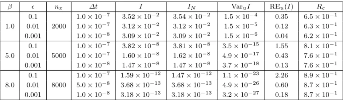
with parameter w = 0.02. The profiles of functions η, V1 and h are shown in Figure 1. Notice that function η is introduced in (4.2) and (4.4) in order that Assumption 1-3 of Theorem 3.1 in Section 3 are satisfied. More discussions on these assumptions can be found in the section of Introduction and Conclusions.
For dynamics (4.1), using the specific form of potentialV, we can obtain that the invariant measure of the fast dynamicsys for each fixedx∈Rhas the density
ρx(y)∝e−β(x−y) 2
(4.5)
with respect to the Lebesgue measure. Also following the discussions in Section 3, especially (3.3) and (3.4), we know the averaged dynamics is a one-dimensional diffusion in a double well potential :
dxes=−V10(exs)ds+β−1/2dws, (4.6) where potentialV1 is given in (4.2) andwsis a one-dimensional Wiener process.
Before we proceed, it is helpful to briefly illustrate the difficulty to compute (4.3) with the standard Monte Carlo method, which is mainly due to system’s metastability when β is mod-erate or relatively large. On one hand, in the path space, the exponential integrand in (4.3) is peaked around trajectories which spend a large portion of time at the minimum ofh, which is located around x= 1 (Figure 1(c)). On the other hand, in order to get close to state x= 1,
trajectories starting from x0 = −1 need to cross the energy barrier ∆V1(≈ V1(0)−V1(−1)) of V1 (Figure 1(b)). The probability of these barrier-crossing trajectories is roughly of order
exp(−β∆V1) whenβ∆V1 is large. Combining these facts, we can conclude that the rare barrier crossing events play an important role when computing (4.3). And standard Monte Carlo method will be inefficient in such a situation due to insufficient sampling of these rare events (cf. the discussion in Section 1).
Computation of the suboptimal estimator based on the averaged equation. Now let us consider the method outlined in Subsection 3.1. Recalling (3.18), the averaged conditional expectationφ0 solves the linear backward evolution equation
∂φ0 ∂t +Leφ0−βehφ0= 0 φ0(T, x) = 1, (4.7) with e L=−V10 ∂ ∂x + 1 2β ∂2 ∂2x, eh(x) =h(x). (4.8)
The equation for φ0 is one-dimensional (in space), and can be solved by standard method: For instance, using Rothe’s method, we can first discretize (4.7) in time, which yields
( 1 ∆t−Le ) φj0= ( 1 ∆t−βh ) φj0+1, j= 0,1,· · ·, m−1 (4.9) whereφj0 denotes the approximation ofφ0 at timetj =j∆t,j= 0,1,· · · , mwith time step size
∆t = T /m. Equation (4.9) is then further discretized in space using the structure-preserving finite volume method described in [31]. Starting from φm
0 ≡ 1, we can obtain all φ
j
0 for j = m−1, m−2,· · ·,1 by solving (4.9) backwardly.
After obtaining φ0, we can compute the feedback control force (3.8) as ˆ u0s= ( −β−1∂xφ0(s, x u s) φ0(s, xu s) ,0 ) , (4.10)
when system’s state is at (xus, ysu) at times. Plugging the last expression into (4.1) then yields the controlled dynamics (also see (2.7))
dxus =−∂V(x u s, yus) ∂x ds+β −1∂xφ0(s, xus) φ0(s, xus) ds+β−1/2dws1 dysu=−1 ∂V(xu s, yus) ∂y ds+β −1/2√1 dw 2 s, (4.11)
which will be employed to sample (4.3) using the reweighted estimator (2.8).
Numerical results. Now we turn to the numerical results. Table 1 shows the numerical results of the Monte Carlo method with the above importance sampling strategy, i.e. (4.11), which should be compared to Table 2 that shows the result of standard Monte Carlo method. For both the weighted and unweighted estimates, the sample size was set toN = 104trajectories
of lengthT = 1 with time step∆t≤10−7that is chosen small enough to remove discretization
bias. The control (4.10) was obtained by computing φ0 from (4.9) on a grid of size nx. For comparison, we have computed a reference importance sampling Monte-Carlo solution (“exact”
−4 −2 x0 2 4 −0.2 0.0 0.2 0.4 0.6 0.8 1.0 η(x) (a) −3 −2 −1 x0 1 2 3 0 1 2 3 4 5 6 7 8 V1(x) (b) −4 −2 x0 2 4 0 2 4 6 8 10 12 h(x) (c)
Fig. 1: (a) Functionη(x) used to define potentialV1. (b) Double well potentialV1(x). (c) Function hin (4.3).
mean value) based on N = 105 independent realizations that is displayed in Table 1 in the
column with label “I”. The performance of the Monte Carlo methods can be evaluated based on the variance (2.6) and the relative error (2.10). In our numerical study, they are estimated from the sampled trajectories as
VaruI= 1 N N ∑ i=1 [( exp ( −β ∫ T 0 h(xu,is )ds ) (Ztu,i)−1 ) −IN ]2 , REu(I) = √ VaruI IN , (4.12) where xu,i
s is thei-th trajectories, 1≤i≤N, IN is the estimator (2.8) ofI, and udenotes the control force. See Section 2 for details. Furthermore, in order to illustrate the actual effect of the control force, we monitor the barrier crossing events with xs ≥0 for some 0< s≤T = 1 and letRc record the ratio of trajectories which cross the barrier among all the trajectories.
In Table 1, for different values of β, we can see that the relative error of the importance sampling estimator becomes smaller as decreases from 0.1 to 0.001. This indicates that the importance sampling estimator performs better and better when deceases and therefore is accordance with the conclusion of Theorem 3.1 in Section 3.
It is also worth making a comparison of both the importance sampling estimator and the standard Monte Carlo estimator. For the importance sampling estimator (Table 1), we observed that both the mean values and the variances, estimated with N = 104 trajectories, are stable after we ran several times and are close to the results estimated with N = 105 trajectories,
which we take as the “exact” mean value. For the standard Monte Carlo method (Table 2), at
β = 1, while it gives acceptable mean values, the sample variances (and the relative errors) are larger comparing to the importance sampling estimator. Forβ= 5, 8, however, the results with standard Monte Carlo method become far away from the “exact” mean values and are unstable when we ran several times. These results indicate that the standard Monte Carlo method is inefficient in this situation.
The above results can be better understood if we consider the barrier-crossing events oc-curred during time [0,1]. These events are related to the metastability of the system and become rare forβ = 5 andβ = 8. In the “Rc” column of Table 2, we see that very few trajectories can cross the energy barrier when β = 5, and it becomes even rarer whenβ is further increased to
observation reveals the fact that crossing the energy barrier is a rare event (in the uncontrolled system) due to system’s metastability at moderate temperature. And it also explains why the estimations of the mean values are largely underestimated by the standard Monte Carlo method (compare Table 1 and Table 2). On the other hand, as shown in “Rc” column of Table 1, the barrier-crossing events are much better sampled by the importance sampling estimator. Also Figure 2 shows the control force (4.10) as a function ofxand timesfor various values ofβ. We clearly observe that the control acts against the energy barrier (blue region) and assists the slow variablexsof the system to transit fromx=−1 tox= 1.
We conclude this section with the following remark on some further numerical issues.
Remark 4 1. It is necessary to solve the averaged equation (3.6) forU0, or equivalently (3.18) for
φ0, in order to compute control (3.8). Solvingφ0from (3.18) may be relatively easier because
the equation is linear. Furthermore, since equation (3.18) doesn’t involve small parameter
any more, it can be solved on a coarser grid and the numerical computation is not expensive. 2. In our example, the probability density ρx(y) can be solved analytically and used to obtain averaged dynamics (3.3) or (4.6). More generally, coefficients (3.4) of the averaged dynamics (3.3) could be numerically computed from the time integration of the fast subsystem (3.2). See Chapter 10 -11 of [37] and also [45] for more details.
3. In principle, the method described above for solving linear PDE (4.7) is computationally applicable when the dimensionkof system’s slow variables xis smaller or equal to 3. Alter-native approaches need to be studied for systems with more slow variables. See Conclusions for further discussions.
Table 1: Numerical results for importance sampling Monte Carlo method withT = 1.0. Columns
I and IN are the mean values computed with N = 105 (“exact”) and N = 104, respectively. Columns VaruI,REu(I) display the variance and the relative error defined in (2.6) and (2.10) estimated from trajectories as in (4.12). ColumnRc shows the ratio of the trajectories that have crossed the potential barrier.
β nx ∆t I IN VaruI REu(I) Rc 1.0 0.1 2000 1.0×10⁻⁷ 3.52×10⁻² 3.54×10⁻² 1.5×10⁻⁴ 0.35 6.5×10⁻¹ 0.01 1.0×10⁻⁷ 3.12×10⁻² 3.12×10⁻² 1.5×10⁻⁵ 0.12 6.3×10⁻¹ 0.001 1.0×10⁻⁸ 3.09×10⁻² 3.09×10⁻² 1.5×10⁻⁶ 0.04 6.2×10⁻¹ 5.0 0.1 5000 1.0×10⁻⁷ 3.82×10⁻⁸ 3.81×10⁻⁸ 3.5×10⁻¹⁵ 1.55 8.1×10⁻¹ 0.01 1.0×10⁻⁷ 1.60×10⁻⁸ 1.62×10⁻⁸ 4.9×10⁻¹⁷ 0.43 7.6×10⁻¹ 0.001 1.0×10⁻⁸ 1.47×10⁻⁸ 1.47×10⁻⁸ 3.7×10⁻¹⁸ 0.13 7.6×10⁻¹ 8.0 0.1 8000 1.0×10⁻⁷ 1.59×10⁻¹² 1.47×10⁻¹² 1.1×10⁻²³ 2.26 8.9×10⁻¹ 0.01 5.0×10⁻⁸ 3.68×10⁻¹³ 3.68×10⁻¹³ 4.9×10⁻²⁶ 0.60 8.7×10⁻¹ 0.001 1.0×10⁻⁸ 3.18×10⁻¹³ 3.18×10⁻¹³ 3.2×10⁻²⁷ 0.18 8.7×10⁻¹
5 Proof of the main result
In this section, we prove our main result, Theorem 3.1 in Section 3.1. Since parameterβ is fixed, it can be absorbed into coefficientsα1andα2, h, and we can assumeβ = 1 without loss of
Table 2: Numerical results for standard Monte Carlo method (u= 0). The labels have the same meaning as in Table 1. β ∆t IN VaruI REu(I) Rc 1.0 0.1 1.0×10⁻⁷ 3.58×10⁻² 4.3×10⁻³ 1.83 1.9×10⁻¹ 0.01 1.0×10⁻⁷ 3.27×10⁻² 3.9×10⁻³ 1.91 1.8×10⁻¹ 0.001 1.0×10⁻⁸ 3.14×10⁻² 3.4×10⁻³ 1.86 1.8×10⁻¹ 5.0 0.1 1.0×10⁻⁷ 2.27×10⁻⁸ 6.3×10⁻¹³ 34.97 3.0×10⁻⁴ 0.01 1.0×10⁻⁷ 2.98×10⁻⁹ 6.4×10⁻¹⁶ 8.49 0 0.001 1.0×10⁻⁸ 3.61×10⁻⁹ 6.8×10⁻¹⁵ 22.84 1.0×10⁻⁴ 8.0 0.1 1.0×10⁻⁷ 3.68×10⁻¹⁴ 1.1×10⁻²⁴ 28.50 0 0.01 5.0×10⁻⁸ 1.87×10⁻¹⁴ 3.8×10⁻²⁵ 32.96 0 0.001 1.0×10⁻⁸ 2.01×10⁻¹⁴ 4.4×10⁻²⁵ 33.00 0
−3 −2 −1 0 1 2 3
0.0
0.2
0.4
0.6
0.8
1.0
tim
e
β =1.0
−3 −2 −1 0 1 2 3
β =5.0
−3 −2 −1 0 1 2 3
β =8.0
−3.5 −3.0 −2.5 −2.0 −1.5 −1.0 −0.5 0.0
0.5
Fig. 2:x-component of control force ˆu0
sdefined in (4.10) for differentβ as function ofxand time
s.
generality. Also recall thatk · kdenotes the Frobenius norm of matrices and| · |is the Euclidean norm of vectors or the absolute value of a scalar.
Our analysis is based on the solution φ of the linear backward evolution equation (3.14) and the solutionφ0 of (3.18) where, by Feynman-Kac formula, bothφandφ0can be expressed in terms of conditional expectations like (3.20).
Idea of the proof. Under Assumption 1, it is well known that bothφ and φ
0 are C1
explicit representation formulas in terms of conditional expectations : ∂xiφ =−Ex,y[e−∫tTh(xs)ds ∫ T t ∇xh(xs)·xs,xids ] , 1≤i≤k ∂yiφ =−Ex,y[e−∫T t h(xs)ds ∫ T t ∇xh(xs)·xs,yids ] , 1≤i≤l ∂xiφ0=−E x[e−∫tTh(exs)ds ∫ T t ∇xh(xes)·xes,xids ] , 1≤i≤k . (5.1)
That is, the derivatives can be put inside the expectation, see Section 1.3 of [8] and Section 2.7-2.8 of [30]. Here, we have used Assumption 3 that the running cost hdepends only on x, and that dynamicsxs, ysandxessatisfy (3.1) and (3.3). Moreover, we have employed the shorthand
Ex,y to denote the expectation conditioned onxt=x, yt=y and similarly forEx. Processesxs,xi ∈R
k, y
s,xi ∈R
lin (5.1) describe the partial derivatives of processesx sand
ys with respect to the initial conditions and satisfy dynamics
dxs,xi= (∇xf xs,xi+∇yf ys,xi)ds+ (∇xα1xs,xi+∇yα1ys,xi)dw 1 s dys,xi = 1 (∇xg xs,xi+∇yg ys,xi)ds+ 1 √ (∇xα2xs,xi+∇yα2ys,xi)dw 2 s 1≤i≤k (5.2) with xjt,x i =δij,1≤j ≤k, yt,xi = 0∈R l. In the above ∇
xα1xs,xi denotes the k×m1 matrix
whose components are
(∇xα1xs,xi)j1j2 = k ∑ r=1 ∂(α1)j1j2 ∂xr xrs,xi, 1≤j1≤k , 1≤j2≤m1, (5.3)
and the meanings of other terms are similar. Analogously, processes xs,yi ∈ R
k andy
s,yi ∈R
l satisfy
dxs,yi = (∇xf xs,yi+∇yf ys,yi)ds+ (∇xα1xs,yi+∇yα1ys,yi)dw
1 s dys,yi = 1 (∇xg xs,yi+∇yg ys,yi)ds+ 1 √ (∇xα2xs,yi+∇yα2ys,yi)dw 2 s 1≤i≤l (5.4) with xt,yi = 0 ∈ R k, yj t,yi = δij ∈ R
l,1 ≤ j ≤ l (Notice that the above dynamics also hold when coefficient α1 depends on bothx, y, so terms involving∇yα1 are kept there). The above formulas (5.1)–(5.4) will allow us to compare the dynamicsxs, ys,xes, the controlled dynamics and the resulting importance sampling estimators. For simplicity, we consider the dynamics on [0, T] that entails similar estimates for the case s∈[t, T]. We therefore suppose that the initial values of xs,xes are x0 ∈Rk and the initial value of ys is y0 ∈ Rl. The notation E below will always refer to expectation conditioned on these initial values.
To prove Theorem 3.1, we will adapt some estimates used in [32]. Also see [10, 8, 26, 21] for similar techniques. To this end, we follow [32] and define a partition of the interval [0, T] by [0, ∆], [∆,2∆],· · ·, [(M−1)∆, M ∆] with∆=T /M,M >0, and consider the auxiliary process
dˆxs=f(xj∆,yˆs)ds+α1(xs)dws1 dyˆs= 1 g(xj∆,yˆs)ds+ 1 √ α2(xj∆,yˆs)dw 2 s (5.5)
fors∈[j∆,(j+ 1)∆), 0≤j≤(M −1), with the continuity condition ˆ
x(j+1)∆= lim
s→(j+1)∆−xˆs, y(ˆj+1)∆=s→(limj+1)∆−yˆs,
and initial conditions ˆx0=x0, ˆy0=y0. Without loss of generality, we can suppose that∆≤1. This auxiliary process will serve as a bridge between (3.1) and (3.3). In contrast to [32] and owed to the fact that we consider controlled dynamics, estimates for 4th-order moments as well as for the processes (5.2) and (5.4) will be needed in order to prove the theorem.
Before entering the details of the various estimates, we first summarize our main technical results, the proofs of which will be given in the following subsections.
For the derivative processes satisfying (5.2) and (5.4), we have (see Theorem 5.6 and Lemma 5.4 below):
Theorem 5.1 Let Assumptions 1–3 hold. Then ∃C >0, independent of ,x0 andy0, such that
max 0≤s≤TE|xs,xi| 2≤C, max 0≤s≤TE|ys,xi| 2≤C, 1≤i≤k. max 0≤s≤TE|xs,yi| 2≤C2, E|y t,yi| 2≤e−λt +C2, t∈[0, T], 1≤i≤l.
For the approximation results, we have (see Theorem 5.7 and Theorem 5.8 below):
Theorem 5.2 Let Assumptions 1–3 hold. Then ∃C > 0, independent of and can be chosen uniformly forx0,y0 which are contained in some bounded domain ofRk×Rl, such that
max
0≤s≤TE|xs−xes|
4≤C1 2.
Theorem 5.3 Let Assumptions 1–3 hold. Then ∃C > 0, independent of and can be chosen uniformly forx0,y0 which are contained in some bounded domain ofRk×Rl, such that
max
0≤s≤TE|xs,xi−xes,xi|
2≤C1 4.
From these results that will be proved in the remainder of this section, we then obtain:
Theorem 5.4 Let Assumptions 1–3 hold. Then ∃C > 0, independent of and can be chosen uniformly forx,y which are contained in some bounded domain ofRk×Rl, such that
1. |∇yφ| ≤C, |∇xφ− ∇xφ0| ≤C 1 8. 2. ForU=−logφ,U 0=−logφ0, we have |∇yU| ≤C, |∇xU− ∇xU0| ≤C 1 8. (5.6)
Proof We use representation formulas (5.1). For ∇yφ, using Assumption 1 and Theorem 5.1, we have |∂yiφ | ≤E(e−∫tTh(xs)ds ∫ T t |∇xh(xs)||xs,yi|ds ) ≤CE ∫ T t |xs,yi|ds≤C ∫ T t (E|xs,yi| 2)1 2ds≤C . To compare∇xφwith ∇xφ0, we compute that
|∂xiφ −∂ xiφ0| ≤E [ e−∫tTh(xs)ds ( ∫ T t ( ∇xh(xs)·xs,xi− ∇xh(exs)·xes,xi ) ds)] +E [( e− ∫T t h(xs)ds−e− ∫T t h(exs)ds )( ∫ T t ∇xh(xes)·exs,xids )] =I1+I2.
ForI1, using Assumption 1, Theorem 5.2 and Theorem 5.3, it follows that I1≤E ( ∫ T t ( ∇xh(xs)·xs,xi− ∇xh(exs)·xes,xi ) ds) =E ( ∫ T t [( ∇xh(xs)− ∇xh(xes) ) ·xs,xi+∇xh(xes)·(xs,xi−exs,xi) ] ds) ≤CE [ ∫ T t ( |xs−xes||xs,xi|+|xs,xi−xes,xi| ) ds ] ≤C ∫ T t [( E|xs−xes|2 )1 2(E|x s,xi| 2)12 +(E|x s,xi−exs,xi| 2)12 ] ds≤C18 . ForI2, we have I2≤ [ E ( e−∫tTh(xs)ds−e− ∫T t h(exs)ds )2]1 2[ E ( ∫ T t ∇xh(xes)·exs,xids )2]1 2 ≤C { E [ ∫ 1 0 e−∫tT(1−r)h(xs)+rh(exs)ds ( ∫ T t |h(xes)−h(xs)|ds ) dr ]2}1 2( E ∫ T t |xes,xi| 2ds) 1 2 ≤C ( E ∫ T t |exs−xs|2ds )1 2 ≤C18,
which then entails the estimates for the derivatives ofφ. Meanwhile, using a similar argument,
|φ−φ0|=E ( e−∫tTh(xs)ds−e− ∫T t h(exs)ds) ≤E [ ∫ 1 0 e−∫tT(1−r)h(xs)+rh(exs)ds ( ∫ T t |h(xes)−h(xs)|ds ) dr ] ≤CE ( ∫ T t |h(exs)−h(xs)|ds ) ≤C ∫ T t ( E|xes−xs|4 )1 4ds≤C18.
Since h is bounded by Assumption 1, we have e−C(T−t) ≤ φ ≤ eC(T−t) is uniformly
bounded (and bounded away from zero) for all > 0. The conclusion concerning |∇yU| and
Recall that, in Section 2 and Subsection 3.1, ˆuis the optimal control as given by (2.16) and that the control ˆu0 defined in (3.8) is a candidate for the suboptimal control which is used for
estimating (2.1) with nearly optimal variance. Theorem 3.1 that is entailed by the above results expresses this fact, and we restate it for the readers’ convenience:
Theorem 5.5 Let Assumptions 1–3 hold, and consider the importance sampling method for computing (2.1) under the dynamics (3.1). When the control uˆ0 as given in (3.8) is used to perform the importance sampling, the relative error (2.10) of the Monte Carlo estimator satisfies
REuˆ0(I)≤C 1 8
for1 whereC >0 is a constant independent of.
Proof In the following we will regard the optimal control ˆu and control ˆu0 as functions of t, x
andy. Using (2.16) and (3.8), we see that Theorem 5.4 implies that |uˆs−uˆ0s| ≤C 1
8 uniformly on [0, T]×D whereD is any bounded domain ofRk×Rl and constant C depends on domain
D. Furthermore, both of them are uniformly bounded on [0, T]×Rk×Rlfrom the boundedness ofφ, α1, α2 and formula (5.1).
Now call ˜x¯us,y˜¯suthe controlled dynamics of (3.1) corresponding to the control ˜u¯s= 2ˆus−uˆ0s. Specifically, using (2.16) and (3.8) again, we have (forβ = 1 and assume Assumption 3)
dx˜¯us =f(˜x¯us,y¯˜us)ds−α1(˜x¯us)α T 1(˜x¯ u s)(2∇xU(˜x¯us,y˜¯ u s)− ∇xU0(˜x¯su)) +α1(˜x¯us)dw 1 s dy˜¯su= 1 g(˜x¯ u s,y˜¯su)ds− 2 α2(˜x¯ u s,y˜¯su)αT2(˜x¯us,y˜¯su)∇yU(˜x¯us,y˜¯us) + 1 √ α2(˜¯x u s,y˜¯us)dws2, (5.7)
and control ˜u¯s is bounded on [0, T]×Rk ×Rl uniformly for . This especially implies that Lemma 5.2 and Lemma 5.3 in Subsection 5.2 also hold for dynamics ˜x¯u
s,y˜¯us (see Remark 6). Let R > 0 and for y ∈ Rl, we define χ
R(y) = 1, if |y| ≤ R, and χR(y) = 0 otherwise. Similarly, for x ∈ Rk, y ∈ Rl, we define χR(x, y) = 1, if both |x|,|y| ≤ R, and otherwise
χR(x, y) = 0. Then applying the uniform approximation|uˆs−uˆ0s| ≤CR 1
8 on bounded domain defined byχR(x, y) and the boundedness of both controls, we can recast (2.20) as
˜ ¯ E [ exp ( ∫ T t |uˆs−uˆ0s| 2χ R(˜x¯us,y˜¯ u s)ds+ ∫ T t |uˆs−uˆ0s| 2(1−χ R(˜x¯us,y˜¯ u s) ) ds )] ≤eCR(T−t) 1 4˜¯ E [ exp ( ∫ T t |uˆs−uˆ0s| 2(1−χ R(˜x¯us,y˜¯ u s))ds )] ≤eCR(T−t) 1 4˜¯ E [ exp ( C ∫ T t (1−χR(˜x¯su,y˜¯us))ds )] ≤eCR(T−t) 1 4[ eCδ+eCTP ( ∫ T t (1−χR(˜x¯us,y˜¯ u s))ds≥δ )] (5.8)
where δ >0 andCR is a constant that depends on R >0. In the last inequality we have split the expectation according to event{∫tT(1−χR(˜x¯su,y˜¯us))ds≥δ}and its complement. Therefore, applying the conclusion of Lemma 5.3 to processes ˜¯xu
s,y˜¯us, we can bound the above quantity (5.8) by eCR(T−t) 1 4[ eCδ+eCTCT(1 +|x| 4+|y|4) δR4 ] .
Now we can first choose a smallδ and then a largeRsuch that ˜ ¯ E [ exp ( ∫ T t |uˆs−uˆ0s|2ds )] ≤2eC(T−t) 1 4
where constantC >0 is independent of. Combing this with (2.6) and (2.10), we conclude that REuˆ0(I)≤C
1 8
wheneveris sufficiently small. ut
5.1 Estimates for processesxs,yi andys,yi
We first consider processes xs,yi and ys,yi in (5.4), since the arguments are simpler and largely
unrelated to the rest of the proof. In the following and throughout this section, we denote byC
a generic constant that is independent ofand whose value may change from line to line.
Lemma 5.1 Under Assumptions 1–2, there existsC >0, independent of,x0 andy0, such that
max 0≤s≤TE|xs,yi| 2≤C, E|y t,yi| 2≤e−λt +C, t∈[0, T], 1≤i≤l. (5.9)
Proof Recall the notation in (5.3) and apply Ito’s formula to |xs,yi|
2 and |y
s,yi|
2. After taking
expectation, equation (5.4) yields
dE|xs,yi|
2= 2Eh∇
xf xs,yi, xs,yiids+ 2Eh∇yf ys,yi, xs,yiids+Ek∇xα1xs,yi+∇yα1ys,yik
2ds dE|ys,yi| 2=2 Eh∇xg xs,yi, ys,yiids+ 2 Eh∇yg ys,yi, ys,yiids+ 1 Ek∇xα2xs,yi+∇yα2ys,yik 2ds , (5.10)
wherek·kdenotes the Frobenius norm of a given matrix. Then, using Cauchy-Schwarz inequality, Lipschitz continuity of the coefficients (Assumption 1) and inequality (3.11) in Remark 2, it follows that dE|xs,yi| 2 ds ≤C ( E|xs,yi| 2+E|y s,yi| 2) dE|ys,yi| 2 ds ≤ − λ E|ys,yi| 2+C E|xs,yi| 2 (5.11) withE|x0,yi| 2= 0,E|y0 ,yi|
2= 1. The conclusion then follows from Claim A.1 in Appendix A. ut
The above result can be improved if we additionally impose Assumption 3 and if we treat the initial layer neart= 0 more carefully.
Theorem 5.6 Let Assumptions 1–3 hold. Then ∃C >0, independent of ,x0 andy0, such that
max 0≤s≤TE|xs,yi| 2≤C2, E|y t,yi| 2≤e−λt +C2, t∈[0, T], 1≤i≤l .
Proof Applying Ito’s formula in the same way as in Lemma 5.1 and noticing that now coefficient
α1is independent ofy, we can obtain dE|xs,yi|
2= 2Eh∇
xf xs,yi, xs,yiids+ 2Eh∇yf ys,yi, xs,yiids+Ek∇xα1xs,yik
2ds dE|ys,yi| 2=2 Eh∇xg xs,yi, ys,yiids+ 2 Eh∇yg ys,yi, ys,yiids+ 1 Ek∇xα2xs,yi+∇yα2ys,yik 2ds . (5.12)
Now set t1=−2λln and introduce the functionη: [0, T]→[0,1] by
η(t) = { 1−tt 1 0≤t≤t1 0 t1< t≤T (5.13)
Then using Cauchy-Schwarz inequality and Lipschitz condition in Assumption 1, we have
Eh∇yf ys,yi, xs,yii ≤C ( −η(s)E|xs,yi| 2 2 + η(s)E|ys,yi| 2 2 ) Eh∇yg xs,yi, ys,yii ≤ C2 λ E|xs,yi| 2 2 +λ E|ys,yi| 2 2 .
Substituting them into (5.12) and apply inequality (3.11) in Remark 2, we can obtain
dE|xs,yi| 2 ds ≤C(1 + −η(s))E|x s,yi| 2+Cη(s)E|y s,yi| 2 dE|ys,yi| 2 ds ≤ − λ E|ys,yi| 2+C E|xs,yi| 2 withE|x0,yi| 2= 0, E|y0 ,yi|
2= 1. The conclusion follows from Claim A.2 in Appendix A. ut
5.2 Stability estimates
We start with some basic facts related to the stability of the dynamics (3.1), (3.3), (5.2) and (5.5). Bear in mind thatβ = 1 throughout this section. For processesxs, ys satisfying (3.1), we have:
Lemma 5.2 Under Assumption 1, 2, there exists C >0, independent of,x0 andy0, such that
max
0≤s≤TE|xs|
4≤C(|x0|4+|y0|4+ 1), max 0≤s≤TE|ys|
4≤C(|y0|4+|x0|4+ 1). (5.14)
Proof Applying Ito’s formula to|xs|4 and taking expectation, we can obtain
dE|xs|4 ds =4E ( |xs|2hf(xs, ys), xsi ) + 2E ( |xs|2kα1(xs, ys)k2 ) + 4E ( |αT1(xs, ys)xs|2 ) ≤4E ( |xs|2hf(xs, ys), xsi ) + 6E ( |xs|2kα1(xs, ys)k2 ) ,
and similarly for|ys|4,
dE|ys|4 ds ≤ 4 E ( |ys|2hg(xs, ys), ysi ) +6 E ( |ys|2kα2(xs, ys)k2 ) .