POUR L'OBTENTION DU GRADE DE DOCTEUR ÈS SCIENCES
acceptée sur proposition du jury: Prof. T. Mountford, président du jury Prof. A. C. Davison, Prof. J. Tawn, directeurs de thèse
Dr Ph. Naveau, rapporteur Dr P. Northrop, rapporteur Prof. S. Morgenthaler, rapporteur
Semiparametric Bayesian
Risk Estimation for Complex Extremes
THÈSE N
O8349 (2018)
ÉCOLE POLYTECHNIQUE FÉDÉRALE DE LAUSANNE
PRÉSENTÉE LE 26 AVRIL 2018À LA FACULTÉ DES SCIENCES DE BASE CHAIRE DE STATISTIQUE
PROGRAMME DOCTORAL EN MATHÉMATIQUES
Suisse 2018 PAR
μηδὲν ἄγαν
(inscription on the temple of Apollo at Delphi)
Acknowledgements
I am much indebted to Anthony Davison, who provided me with the support for carrying research in an excellent environment, giving the opportunity for me to participate in many international conferences and workshops. I learned a lot from his broad knowledge, patience and kindness. His rigour and expertise will continue guiding me in the future.
It is hard to express in a few words how much I owe to Jonathan Tawn, whose tireless energy and motivation steered me throughout my research. He made me feel as if I had always been at Lancaster University, encouraging me to take part in the academic activities of the STOR-i doctoral training centre, that have greatly enriched me. During my many visits to Lancaster, I was able to get ahead in my research, punctuated by very regular meetings with Jon and the inevitable pile of notes —full of ideas— that I would bring back at my desk.
I would also like to thank Paul Northrop, Philippe Naveau, Stephan Morgenthaler, and Thomas Mountford for sitting on the thesis jury and for their careful reading and detailed comments.
I acknowledge support from the Swiss National Science Foundation. Ich möchte mich besonders bei Georges Klein bedanken, denn er hat mich für meine 6-Monaten Besuch in Lancaster wegen der Universitätgebühren ganz nett und professionnell unterstüzt.
I would like to thank Kim and Rosemary, who helped me settle in at STOR-i. It would be too long here to mention all the people in Lancaster with whom I had so many fruitful discussions and spent such a great time; Jenny Wadsworth and Ioannis Papastathopoulos for the helpful discussions, and STOR-i mates Aaron & Jamie-Leigh and their inimitable accents, Christian, Ciara for guiding me through British life and habits, Dave & Aisha for their hospitality, Harjit and his endless theories, Hugo for extreme conversations and the Eurovision, and Charlotte, Jack for the muddy runs, and Sorcha, Jamie and his questions about French words, Lucy for organising outings, Matt & Helen, Paul & Zak, Rhian & Jeddy, Sam for the dry hikes, Kathryn for the Lindy-Hop. My thanks also go to Amy Cotterill for introducing me to the Lakes and the Dales.
J’aimerais également remercier mes collègues et amis de l’EPFL pour leur présence quoti-dienne et les discussions enrichissantes, parmi lesquels Miguel pour m’avoir donné le goût des statistiques bayésiennes non-paramétriques, Claudio pour tous les échanges, Raphaël pour la course à pieds, Léo, Hélène, Peiman, Sophie pour son rayonnement, Sebastian pour son accent vaudois. Je remercie les membres des autres chaires de statistiques, en particulier Rémy, Marie-Hélène et Yoav. Merci beaucoup à Nadia pour son travail efficace et sa disponibilité, et les échanges passionnants.
vi Acknowledgements
Je dois aussi énormément au professionalisme, au calme et à la patience du docteur Duccio Boscherini et de toute son équipe, pour m’avoir remis sur pieds si impeccablement et si rapidement d’une hernie discale qui a si brusquement interrompu ma thèse.
Je pense également aux amitiés forgées dans le travail et les cafés: David, Pauline et Reda, et aux amitiés partagées depuis plus longtemps: Adrien, Denis, Odile, Matthieu et Marie, pour tous les bons moments passés ensemble, les partages, les échanges d’idées et les voyages.
Do të doja të falenderoja zemrën time që më ka nxitur shumë e më ka dhënë besim. Anjeza më ka hapur shpirtin dhe më ka bërë të zbuloj një tjetër botë, plot me bujari. Faleminderit dielli im që ndriçon çdo ditë!
Je pense aussi à mes frères, avec qui j’ai très tôt partagé ce besoin d’expliquer le pourquoi et le comment, et avec certains desquels j’ai eu la chance de partager le quotidien du campus. Merci de tout cœur à ma maman qui a fait de moi ce que je suis, qui m’a constamment soutenu et m’a donné sa confiance inconditionnelle et infrangible. Certes la théorie des nœuds m’est bien trop étrangère pour avoir pu prétendre poursuivre ta recherche interrompue, mais je suis très heureux d’avoir pu t’emboîter le pas dans un autre domaine des mathématiques.
Abstract
Extreme events are responsible for huge material damage and are costly in terms of their human and economic impacts. They strike all facets of modern society, such as physical infrastructure and insurance companies through environmental hazards, banking and finance through stock market crises, and the internet and communication systems through network and server overloads. It is thus of increasing importance to accurately assess the risk of extreme events in order to mitigate them. Extreme value theory is a statistical approach to extrapolation of probabilities beyond the range of the data, which provides a robust framework to learn from an often small number of recorded extreme events.
In this thesis, we consider a conditional approach to modelling extreme values that is more flexible than standard models for simultaneously extreme events. We explore the sub-asymptotic properties of this conditional approach and prove that in specific situations its finite-sample behaviour can differ significantly from its limit characterisation.
For modelling extremes in time series with short-range dependence, the standard peaks-over-threshold method relies on a pre-processing step that retains only a subset of obser-vations exceeding a high threshold and can result in badly-biased estimates. This method focuses on the marginal distribution of the extremes and does not estimate temporal extremal dependence. We propose a new methodology to model time series extremes using Bayesian semiparametrics and allowing estimation of functionals of clusters of extremes. We apply our methodology to model river flow data in England and improve flood risk assessment by explicitly describing extremal dependence in time, using information from all exceedances of a high threshold.
We develop two new bivariate models which are based on the conditional tail approach, and use all observations having at least one extreme component in our inference procedure, thus extracting more information from the data than existing approaches. We compare the efficiency of these models in a simulation study and discuss generalisations to higher-dimensional setups.
Existing models for extremes of Markov chains generally rely on a strong assumption of asymptotic dependence at all lags and separately consider marginal and joint features. We introduce a more flexible model and show how Bayesian semiparametrics can provide
viii Abstract
a suitable framework allowing simultaneous inference for the margins and the extremal dependence structure, yielding efficient risk estimates and a reliable assessment of uncertainty.
Key words:Asymptotic independence; Clustering; Conditional extremes; Dirichlet pro-cess mixture; Extreme value theory; Flood; Hierarchical Bayesian semiparametric inference; Markov chain Monte Carlo; Penultimate analysis; Risk assessment; River flow; Threshold-based extremal index; Time series extremes
Résumé
Les événements extrêmes causent de très importants dégâts matériels et ont un coûteux impact tant humain qu’économique. Ils touchent toutes les facettes de la société moderne, telles les infrastructures matérielles et les compagnies d’assurances par les catastrophes naturelles, le secteur bancaire et le monde de la finance par les crises boursières, ainsi que l’internet et les systèmes de communication par les surcharges des réseaux et des serveurs. Il devient donc toujours plus important d’évaluer le risque d’événements extrêmes avec précision, de manière à pouvoir les anticiper. La théorie des valeurs extrêmes est une approche statistique permettant l’extrapolation de probabilités par-delà les données observées, et fournissant un cadre robuste pour tirer parti d’un nombre souvent restreint d’événements extrêmes enregistrés.
Dans cette thèse, nous considérons la modélisation des valeurs extrêmes par une approche conditionnelle, plus flexible que les modèles standard portant sur les événements extrêmes simultanés. Nous explorons les propriétés sous-asymptotiques de cette approche condition-nelle et démontrons qu’un échantillon fini peut, dans certaines situations, se comporter très différemment de sa caractérisation asymptotique.
Pour la modélisation des extrêmes de séries chronologiques avec de la dépendance à court terme, la méthode usuelle des « pics au-dessus d’un seuil » repose sur un pré-traitement des dépassements d’un seuil élevé qui n’en retient qu’un sous-ensemble et peut conduire à des estimations particulièrement biaisées. Cette méthode se concentre sur la distribution marginale des extrêmes et ne permet pas d’estimer la dépendance temporelle extrémale. Nous développons une nouvelle méthodologie de modélisation des extrêmes de séries chronolo-giques utilisant une approche bayésienne semi-paramétrique, et permettant l’estimation de fonctionnelles de grappes de valeurs extrêmes. Nous appliquons notre méthodologie à la mo-délisation du débit de rivières en Angleterre et améliorons l’évaluation du risque d’inondation en décrivant explicitement la dépendance temporelle extrémale et en exploitant l’information de tous les dépassements d’un seuil élevé.
Nous développons deux nouveaux modèles bivariés basés sur l’approche conditionnelle pour les extrêmes et utilisant pour l’inférence toutes les observations possédant au moins une composante extrême, permettant ainsi d’extraire plus d’information des données que
x Résumé
les approches existantes. Nous comparons l’efficience de ces modèles par des simulations et discutons la généralisation à des dimensions supérieures.
Les modèles de chaînes de Markov pour les extrêmes reposent généralement sur une hypothèse forte de dépendance asymptotique entre tous les événements extrêmes de la chaîne et considèrent les caractéristiques marginale et conjointe de manière distincte. Nous présentons un modèle plus flexible et montrons comment une approche bayésienne semi-paramétrique peut fournir un cadre adapté à l’inférence simultanée des structures extrémales marginale et conjointe, produisant des estimations efficientes du risque et une évaluation fiable de l’incertitude.
Mots-clefs :Analyse de risque ; Analyse sous-asymptotique ; Débit de rivière ; Extrêmes conditionnels ; Extrêmes de séries chronologiques ; Indépendence asymptotique ; Indice extré-mal sous-asymptotique ; Inférence semi-paramétrique bayésienne hiérarchique ; Inondation ; Mélange de processus de Dirichlet ; Méthode de Monte Carlo par chaînes de Markov ; Mise en grappes ; Théorie des valeurs extrêmes
Contents
Acknowledgements v
Abstract vii
Résumé ix
List of figures xiv
List of tables xvi
List of algorithms xvii
1 Introduction 1 1.1 Motivation . . . 1 1.2 Thesis outline . . . 3 2 Modelling extremes 7 2.1 Extrapolation principle . . . 7 2.1.1 Univariate setting . . . 7
2.1.2 Bivariate and low-dimensional setting . . . 9
2.2 Extremes in time series . . . 12
2.3 Modelling asymptotic independence . . . 15
2.3.1 Classification of limit distributions . . . 15
2.3.2 From asymptotic dependence to asymptotic independence . . . 18
2.3.3 Regular variation along rays in exponential margins . . . 20
2.4 Conditional extremes . . . 20
2.4.1 Characterising the limit . . . 20
2.4.2 Heffernan–Tawn formulation . . . 22
2.4.3 Alternative formulation, extensions and additional constraints . . . 25
2.5 Summary . . . 30
3 The Dirichlet process 31 3.1 Formal definitions . . . 31
3.1.1 The Dirichlet distribution . . . 31
3.1.2 Ferguson’s definition . . . 32 xi
xii Contents
3.1.3 Extension of the Pólya urn scheme . . . 33
3.1.4 Constructive definition . . . 33
3.2 The Dirichlet process mixture . . . 34
3.3 Algorithms . . . 35
3.3.1 Marginal approach . . . 35
3.3.2 Conditional approach . . . 37
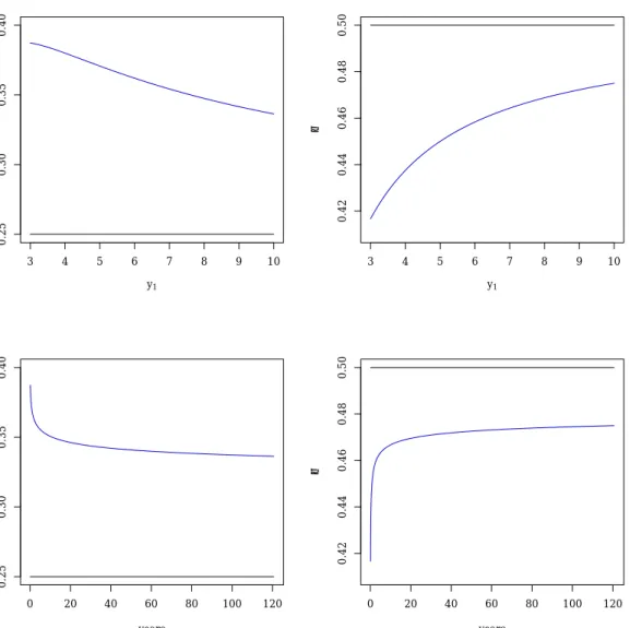
3.4 Example: 3-year bond yields . . . 38
3.5 Summary . . . 42
4 Penultimate analysis of the conditional tail model 45 4.1 Related research . . . 45 4.1.1 Univariate case . . . 45 4.2 Bivariate case . . . 47 4.2.1 Componentwise maxima . . . 47 4.2.2 Conditional extremes . . . 47 4.3 Gaussian distribution . . . 49
4.4 Inverted logistic distribution . . . 55
4.5 Logistic distribution . . . 60
4.6 Summary . . . 62
5 Bayesian uncertainty management in temporal dependence of extremes 63 5.1 Foreword . . . 63
5.2 Introduction . . . 63
5.3 Multivariate setup and classical models . . . 67
5.4 Threshold-based model for conditional probabilities . . . 69
5.4.1 Heffernan–Tawn model . . . 69
5.4.2 Existing inference procedure . . . 71
5.5 Modelling dependence in time . . . 73
5.6 Bayesian Semiparametrics . . . 74
5.6.1 Overview . . . 74
5.6.2 Dirichlet process mixtures for the residual distribution . . . 75
5.6.3 Multivariate semiparametric setting . . . 76
5.6.4 Implementation of existing constraints in the Bayesian framework . . . 77
5.6.5 Implementation issues . . . 79 5.7 Simulation study . . . 80 5.7.1 Bivariate data . . . 80 5.7.2 AR(1) process . . . 81 5.8 Data analysis . . . 84 5.9 Summary . . . 86
6 New improvements to the conditional tail model 89 6.1 Joint likelihood for bivariate extremes . . . 89
Contents xiii
6.2.1 General framework . . . 92
6.2.2 Likelihood contributions averaged inR11 . . . 94
6.2.3 Likelihood contributions split inR11. . . 95
6.2.4 Full methodology including the margins . . . 96
6.3 Inference . . . 98
6.3.1 Strong exchangeability and Gaussian residuals . . . 98
6.3.2 Estimation of conditional quantiles . . . 101
6.3.3 Generalisations and extensions . . . 101
6.4 New constraints for the conditional tail model . . . 103
6.4.1 Existing fitting procedure . . . 103
6.4.2 New constraints under positive and negative association . . . 104
6.5 Improving self-consistency of the conditional tail model . . . 105
6.6 Simulation study . . . 107
6.6.1 Simulation processes . . . 107
6.6.2 Fixed margins . . . 108
6.6.3 Joint fit . . . 111
6.6.4 Conditional quantile constraints . . . 114
6.6.5 Conditional mean constraint . . . 115
6.7 Summary . . . 117
7 Modelling extremes of Markov chains 119 7.1 Background . . . 119
7.1.1 Existing approaches . . . 119
7.1.2 Modelling time series extremes with the conditional tail approach . . . . 120
7.2 Bayesian semiparametrics for modelling first-order Markov chains . . . 120
7.2.1 General . . . 120
7.2.2 Pólya urn scheme . . . 121
7.2.3 Likelihood function . . . 122
7.2.4 Posterior assignment probabilities . . . 124
7.3 Summary and future work . . . 125
8 Discussion and extensions 127
Appendices 131
A Marginal approach to fitting Dirichlet process mixtures 133
B Concentration parameter update 135
C List of bond yields and ratings by country 137
D Penultimate approximation in the univariate case 139 E Posterior densities for the semiparametric model 141
xiv Contents
F State-dependent proposal distribution for(α,β) 143
G Proof of Theorem 6.2 147
H Numerical approach to estimating joint tail probabilities 151 I State-dependent proposal distribution for batch updates 155
Bibliography 158
List of Figures
1.1 Costs (million CHF, inflation-adjusted) of damage caused by floods, debris flows, landslides and rock falls in Switzerland from 1972 to 2016. . . 2 2.1 Data from a bivariate Gaussian copula on four different marginal scales. . . 11 2.2 Novartis and Roche daily stock prices and returns. . . 17 2.3 Estimates ofχ(u) andχ(u) with 95% confidence intervals for Roche and Novartis
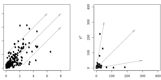
negative returns. . . 17 2.4 Directions of extrapolation for probabilities of extreme sets on exponential and
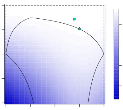
Pareto scales using the Ledford–Tawn formulation. . . 19 2.5 Examples of dependence structures with asymptotic independence spanned by
the conditional model. . . 26 2.6 Constraints on the parameters of the conditional model based on the negative
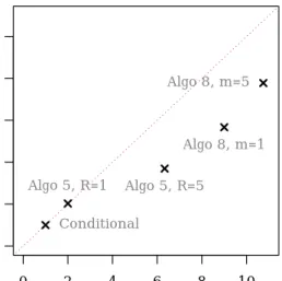
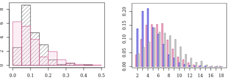
returns of Goldman Sachs, conditioned on big negative returns of Citigroup. . . 28 3.1 Bond yields for 53 countries for a 3-year horizon. . . 39 3.2 Efficiency of Dirichlet process fitting algorithms. . . 41 3.3 Conditional approach to fitting the Dirichlet process: posterior distribution of
the density and distribution functions. . . 41 3.4 Posterior features of the Dirichlet process. . . 42 4.1 Comparison of first- and second-order approximations to the Heffernan–Tawn
parametersαandβfor a Gaussian copula with covariance parameterρ=0.5. . 54 5.1 Comparison of the empirical, stepwise and Bayesian semiparametric estimates
ofθ(x,4). . . 68 5.2 Results for the simulation study based on the Heffernan–Tawn model with a
bimodal residual distribution with two Laplace components. . . 81 5.3 Ratios (%) of RMSEs computed with estimates ofθ(x,m) for a range of values ofρ. 83 5.4 Coverage error forθ(x,m) computed for confidence levels 0.05,0.1,...,0.95, for
x=98% andx=99.999%, withm=1. . . 84
5.5 Posterior summaries forχj(x), j =1,...,7, withxthe 95%, 99%, and 99.99%
marginal quantiles of the River Ray data. . . 85 6.1 Regions where likelihood contributions differ: average and split approaches. . 93 xv
xvi List of Figures
6.2 Regions where likelihood contributions differ, in a 3-dimensional setup: average and split approaches. . . 103 6.3 Minimum values ofµsatisfying the conditional mean constraint. . . 105 6.4 Diagram of the method of proportions for computing joint tail probabilities of
the type Pr(X>vx,Y >vy). . . 110
6.5 Joint fit of the marginal and dependence features for bivariate Gaussian simu-lated data. . . 116 7.1 Multiple use of data points occurring when fitting dependence structures of
the typeX1,...,Xm |X0=x forx extreme in time series, using the standard
conditional tail model approach. . . 120 F.1 Construction of the state-dependent proposal distribution from a bivariate
Gaussian distribution with independent margins. . . 144 F.2 Details of the construction of the approximate tangent to the support boundary
List of Tables
5.1 Ratios (%) of RMSEs computed with estimates ofθ(x,m). . . 83 5.2 Estimation of the threshold-based extremal indexθ(x,m) (%) for four different
levels ofxandm=1,7 on the Ray River winter flow data, with 95% confidence
intervals. . . 86 6.1 Bias×1000 and relative efficiency forαbandβb. . . 109 6.2 Bias×100 and relative RMSE of the GPD scale and shape parameters. . . 112
6.3 Bias×104, variance×108and relative RMSE of joint probabilities of the type
Pr(X>vx,Y >vy) when simultaneously fitting the marginal and joint
distribu-tions. . . 113 6.4 Efficiency gain (%) on (α,β) from using the constraints of Keefet al.(2013). . . 115 C.1 List of countries with 3-year sovereign bond yield (percentage) in mid-November
2017 and Moody’s credit rating (MCR) at that same time. . . 138
List of Algorithms
2.1 Simulating pairs from the conditional model. . . 25
6.1 Sampling from the conditional distribution givenX=xwithxextreme. . . 102
6.2 Sampling with rejection from multiple conditional models. . . 108
A.1 Partial Gibbs sampler for the Dirichlet process. . . 134
A.2 Gibbs sampler with auxiliary parameters for the Dirichlet process. . . 134
1
Introduction
1.1 Motivation
In Switzerland, floods are the most damaging natural hazards in terms of the costs incurred, as is reported for the year 2007 by Hilkeret al.(2008). Floods have also caused more than a hundred deaths since the mid-20th century, but the number of fatalities dropped in the last few decades (Badouxet al., 2016). The last three extremely damaging events which happened in Switzerland were in October 2000, when Canton Valais experienced a major flood in which 16 people died and material damage amounted to CHF 600 million; in August 2005, a widespread flood caused six deaths and cost more than CHF 3 billion; in August 2007, the River Aare and its tributaries impacted regions in the Plateau, the Jura and the Chablais, with damages of more than CHF 600 million (Spicher, 2017; Hilkeret al., 2009; Pfister, 2009). Figure 1.1 shows the inflation-adjusted costs due to floods, debris flows, landslides and rock falls, in Switzerland during the period 1972–2016 (Swiss Federal Institute for Forest, Snow and Landscape Research WSL, 2016); more than 90% of the costs over this period are due to floods and debris flows.
In the UK, the cost of flood damage exceeds £1 billion per year and is expected to rise significantly in the coming decades (Bennett and Hartwell-Naguib, 2014), and 13 deaths due to flooding have been reported since 2000 (Gummer and Leasom, 2016). Government spending on maintenance and extension of flood defences represents more than £600 million a year (Gummer and Leasom, 2016).
Switzerland and the UK are two examples of countries experiencing recurrent flood events, but many other countries in the world endure much more severe flood damage. In order to assign government spending adequately and to efficiently reduce the impacts of large-scale flooding events, it is thus key to be able to model and predict the likelihood of these extreme events.
Carbon dioxide and other pollutants released by human activity trap huge amounts of energy in the atmosphere. Owing to this increasing surplus of energy, we can expect environ-mental damage of greater magnitude and of wider extent than in the previous century. New
2 Chapter 1. Introduction
Year
Damage cost [million CHF]
0 500 1000 1500 2000 2500 3000 1972 1976 1980 1984 1988 1992 1996 2000 2004 2008 2012 2016
Figure 1.1 – Costs (million CHF, inflation-adjusted) of damage caused by floods, debris flows, landslides and rock falls in Switzerland from 1972 to 2016.
homes tend to be built closer to coastlines and flood areas, as safer points are already occupied by existing buildings. The combined effect of demographics and climate change means that more people and goods are at risk of natural catastrophes. Given these changes, it becomes more and more critical to measure the risk of these extreme events in order to mitigate them.
The theory of extreme values can help better understand and estimate the frequency and magnitude of extreme events and provides tools for assessing the risk of events that have yet never been measured. Statistics of extreme events gives the necessary insight for making appropriate decisions for risk mitigation.
Suppose we measure some phenomenon at regular intervals until we havenstationary observations with finite variance, e.g., a river flow recorded every day in winter over a num-ber of years. The central limit theorem would then suggest, fornsufficiently large, that the distribution of the mean of thenobservations approaches a Gaussian distribution at an−1/2
rate. This theorem justifies the use of the Gaussian distribution in many situations, as diverse as modelling random errors, constructing confidence intervals, and making prediction. The Gaussian distribution is so widely used that it becomes a default distribution for many prac-titioners. When the tail of a process is of interest, rather than its mean, using the Gaussian distribution can yield underestimation of joint tail risks, as was experienced in the banking sector in 2007 (Hartmannet al., 2004). The statistical theory of extreme events provides an analogue to the central limit theorem, which establishes the limit distribution, asn→ ∞, of
1.2 Thesis outline 3
appropriate to adopt an extreme value approach, since averages follow a very different process from that of extremes.
After the first results of the statistics of extremes were established (Fisher and Tippett, 1928; von Mises, 1936; Gnedenko, 1943), applications of the theory appear in Gumbel and Goldstein (1964), where the authors consider two data sets with different dependence proper-ties, namely the oldest age at death for females and males in Sweden, and river discharges at two gauges situated along the Ocmulgee River in Georgia (US). The study of life expectancy is still relevant today, and has recently benefitted from the contributions of Einmahlet al.(2017) and Rootzén and Zholud (2017), leading to different conclusions. River flooding has attracted much attention in the extreme value literature and has been applied to high-dimensional and spatial problems (Katzet al., 2002; Keefet al., 2009a,b; Asadiet al., 2015).
Other environmental applications of extreme value models include extreme rainfall (Coles and Tawn, 1996a,b; Süveges and Davison, 2012; Huser and Davison, 2014; Sharkey and Tawn, 2017), extreme wind speeds (Coles and Walshaw, 1994; Fawcett and Walshaw, 2006a,b; Oesting
et al., 2017), wind storms (Coles, 1993; Northropet al., 2017), wave height and extreme sea surge (de Haan and de Ronde, 1998; Fawcett and Walshaw, 2007), heatwaves (Reichet al., 2014; Winter and Tawn, 2016) and high concentrations of air pollutants (Smith, 1989; Heffernan and Tawn, 2004; Eastoe and Tawn, 2009).
Many applications have contributed to the improvement of risk assessment in the insur-ance and fininsur-ance industries, in particular to dependence modelling of extreme stock market losses (Poonet al., 2003), hedging strategies (Hilalet al., 2011), portfolio risk assessment (Hilal
et al., 2014), estimation of value-at-risk and expected shortfall (Chavez-Demoulinet al., 2005, 2014; Caiet al., 2015), and insurance losses (Embrechtset al., 1997; Rohrbecket al., 2018).
1.2 Thesis outline
The thesis is structured as follows: the following two chapters review existing models, the first being focused towards statistics of extreme values, and the second dealing with a Bayesian approach to nonparametric modelling. The next three chapters cover various devel-opments and contributions of the thesis, and the last chapter discusses potential extensions and interesting future directions of research.
In Chapter 2, we review many methods developed in the literature of extreme value modelling, and we explain how these methods tackle the problem of extrapolating probabilities from moderately extreme sets, where data have been observed, to very extreme sets, typically beyond the range of the data, and corresponding to risk levels of interest. We give a brief introduction to univariate modelling of maxima and of excesses of a high threshold, followed by extreme value modelling for time series, which often exhibit short-range dependence at high levels. We then turn our attention to models for multivariate extreme events, in particular those which can capture a dependence strength weakening as we move further
4 Chapter 1. Introduction
into the joint tail. The conditional model for extremes (Heffernan and Tawn, 2004) has the ability of covering many existing non-parametric and parametric models for extremes while being parsimonious. Although the inference procedure advocated by Heffernan and Tawn is very simple, its efficiency has room for improvement, and in Chapter 5 we develop a method which tackles this issue. The conditional tail model is the main concern of this thesis and is developed along different directions in Chapters 4, 5, 6 and 7.
In Chapter 3, we introduce the Dirichlet process as an approach to nonparametric mod-elling in the Bayesian framework, and discuss extensions of it, namely Dirichlet process mixtures. Two broad approaches exist for fitting these mixtures, both of which are illustrated with specific algorithms. The code to fit these algorithms was developed and optimised for the purpose of this thesis. The respective performances of these algorithms in terms of mixing and computational cost are compared. An illustration with real data gives an insight into the performance and flexibility of these methods. One of these algorithms is used and extended in Chapter 5 and potential applications of Dirichlet process mixtures are explored in Chapter 7. In Chapter 4, we delve into the subasymptotic properties of the conditional model intro-duced in Chapter 2. Penultimate analysis was conducted by Smith (1987) and Gomes (1984, 1994) in the context of univariate extreme values, but consideration of the slow convergence of the distribution of the maxima of a Gaussian distribution already appears in Fisher and Tippett (1928). For the conditional model for extremes, the bivariate Gaussian distribution given one of its margins is large is of particular interest, as its rate of convergence to the limit conditional distribution is notably slow. The penultimate analysis of the conditional tail model is helpful in simulations for evaluation purposes when using sample sizes similar to real data sets. In this context, penultimate approximations of the parameters of the conditional tail model, instead of their respective limit values, which can lie well away from the penultimate true values, can be used as benchmarks. We shall use these penultimate approximations in Chapter 6 to help evaluate the efficiency of one of the new approaches presented there.
In Chapter 5, we present a new approach to modelling the extremes of a stationary time series. In this context, both marginal and dependence features must be described. There are standard approaches to marginal modelling, but long- and short-range dependence of extremes may both appear. In applications, an assumption of long-range independence often seems reasonable, but short-range dependence, i.e., the clustering of extremes, needs attention. The extremal index 0<θ≤1 is a natural limiting measure of clustering, but for wide
classes of dependent processes, including all stationary Gaussian processes, it cannot distin-guish dependent processes from independent processes withθ=1. Eastoe and Tawn (2012)
exploit methods from multivariate extremes to treat the subasymptotic extremal dependence structure of stationary time series, covering both 0<θ<1 andθ=1, through the introduction
of a threshold-based extremal index. Inference for their dependence models uses an inefficient stepwise procedure that has various weaknesses and has no reliable assessment of uncertainty. We overcome these issues using a Bayesian semiparametric approach. Simulations and the
1.2 Thesis outline 5
analysis of a UK daily river flow time series show that the new approach provides improved efficiency for estimating properties of functionals of clusters.
In Chapter 6, we shall introduce a new constraint for the conditional tail model. Previously, based on the initial formulation of Heffernan and Tawn (2004), Keefet al.(2013) derive con-straints on the model parameters, which we shall present in Section 2.4.3 of Chapter 2. These constraints help increase efficiency and remove inconsistency of probabilities extrapolated from the model. Another issue remains which these constraints do not address, namely the lack of identifiability of the model parameters in specific situations. We tackle this by adding a new constraint to the model when positive or negative association can reasonably be assumed. We also develop two models for fitting joint distributions for extremes based on the conditional tail model. This gives a coherent framework for fitting multivariate extremes with at least one component being extreme, whereas the method suggested by Heffernan and Tawn (2004) uses an incorrect likelihood function. Our method adds censored data to the fit and makes simultaneous inference for the extremal marginal and dependence features.
In Chapter 7, we return to the issue of fitting time series extremes of Chapter 5, and we propose a model to fit the extremes of first order Markov chains, so that combined inference can be made on extremal marginal and joint distributions, thus giving a full account of uncertainty of the parameter estimates. We develop a semiparametric Bayesian approach to avoid the strong assumptions needed in Chapter 6, and to give an account of uncertainty on the estimated model and on probabilities derived from the model.
We conclude with a discussion of possible extensions of the results presented in the thesis, and in particular potential future work on a generalisation of the approach of Chapter 5 to the spatial context, which can be of great interest for modelling asymptotically independent data, e.g., environmental data, which generally display decreasing strength in extremal dependence between increasingly distant locations.
2
Modelling extremes
2.1 Extrapolation principle
2.1.1 Univariate setting
The study of extreme values is concerned with predicting the likelihood of potentially damaging events at levels never previously recorded. Statistical methods for estimating the probabilities of occurrence of these events help their users to learn from the history of the most harmful events in order to extend information from these events of moderate intensity towards others of higher magnitude for which information is incomplete or absent. More formally, we need to carefully choose a non-empty moderately extreme setA on which we can rely for extrapolation to a more extreme setBcontaining few or no data points.
In the univariate setting withX1,...,Xniid∼F, this extrapolation paradigm appears clearly.
The founding limit theorem in extreme value theory (Fisher and Tippett, 1928; Gnedenko, 1943) states
Theorem 2.1 (Fisher–Tippett–Gnedenko)
Let X1,...,Xn, n∈N, be independent and identically distributed random variables. Consider the
sequence of maxima Mn=max{X1,...,Xn}, n∈N. If this sequence can be linearly renormalised
as(Mn−an)/bn by sequences of locations(an)and scales(bn)>0in order to converge to a
non-degenerate distribution G(x), then G(x)=exp ½ −³1+ξx−µ σ ´−1/ξ + ¾ , x∈R, (2.1)
with c+=max{c,0}, location parameterµ∈R, shape parameterξ∈Rand scale parameterσ>0;
the case withξ=0is interpreted as the limit asξ→0.
This powerful result suggests modelling the distribution of the maxima of observations for finitenusing the single parametric family of distributionsG(x)=G(x;µ,σ,ξ) in (2.1) as an
approximation ofFn(x). When the distributionFconverges toGin the terms of Theorem 2.1, we say thatFis in the domain of attraction ofGand we denote it byD(G).
8 Chapter 2. Modelling extremes
The extrapolation strategy from setA to setBunderlying inference of extreme values and outlined at the beginning of this section is better explained through the point process representation for extremes (Hsinget al., 1988). Consider the point process with points
Pn= ½µ i n+1, Xi−an bn ¶ :i=1,...,n ¾ . (2.2)
From Theorem 2.1 we have Pr µM n−an bn ≤x ¶ ={F(bnx+an)}n→G(x), n→ ∞ (2.3)
withG(x) non-degenerate, or equivalently on the log scale,
n{1−F(bnx+an)}→ −logG(x), n→ ∞. (2.4)
We get the intensity of the point process (2.2) if we consider the number of excesses ofbnx+an,
as in Leadbetter (1976). More precisely, we considerNn(x)=Pni=11(Xi>bnx+an), whose
distribution is Bin{n,1−F(bnx+an)}. The Poisson limit and (2.4) yield
Nn(x)→N(x)∼Pois{−logG(x)}.
We get the sizes of the excesses ofanx+bn, i.e., the sizes of the marks of (2.2), through the
limit Pr(X>bnx+an|X>an)=1−F(bnx+an) 1−F(an) =n{1−F(bnx+an)} n{1−F(an)} →logG(x) logG(0) = µ 1+ξ x σ−ξµ ¶−1/ξ + , n→ ∞. (2.5)
Asn→ ∞,an→xF, the upper endpoint ofF, suggesting the approximation using the
gener-alised Pareto distribution
Pr(X>x+u|X>u)≈(1+ξx/σu)−+1/ξ, for largeu, (2.6)
whereσu>0 is a scale parameter that is a function of the thresholdu.
We can now depict how extrapolation underlies inference for very extreme sets, as we can derive Pr(X∈B) from Pr(X∈A) and (2.5),
Pr(X∈B)= µ 1+ξv−u σu ¶−1/ξ + Pr(X∈A), withA =[u,∞) andB=[v,∞),u<v.
2.1 Extrapolation principle 9
2.1.2 Bivariate and low-dimensional setting
Coles and Tawn (1994) consider structure variables of interest in practical design prob-lems, reducing the dimension of the problem so that univariate methods of Section 2.1.1 can easily be applied. IfBis an extreme set of interest andX are observed data, the structure variableS(X) transforms the original multivariate problem into the much simpler problem of estimating
Pr(X∈B)=Pr{S(X)>v}.
The authors give several examples of design settings where specific structure variables are of interest. For example, offshore platform engineers are mainly interested in the force of waves
X1and windsX2, and a typical structure variable in this context would beS(X)=S(X1,X2)=
a1X12+a2X22; in rainfall studies for which we have gauges at sitesX1,...,Xd, a quantity of
interest is the cumulative rainfall measured over a whole regionPd
j=1wjXj, withw1,...,wd
being weights associated with the sites. This last structure variable could also be interpreted in the financial context as a portfolio ofdassets where theXjrepresent the negative returns and
for which we are interested in potential extreme losses. The main interest of such an approach is that it only needs a univariate fit without needing to consider the dependence between variables. On the other hand, the structure variable approach does not guarantee coherence between probabilities extrapolated from different structure variables based on the same data; it hides the connections between variables, and is unable to account for deterministic and potentially abrupt changes in the structure ofSbeyond the data.
Consideration of extremes of bivariate and higher-dimensional data entails defining an ordering inRd,d
≥2. Barnett (1976) lists various orderings, a couple of which have been
considered in the literature. The structure variable is one. Standard approaches in extreme value problems use componentwise maxima, which can combine either simultaneous events, e.g., recorded on the same day, or events recorded at different time points. Stephenson and Tawn (2005) raise this issue and suggest distinguishing the contributions depending on which of these two types the observed maxima correspond to.
The univariate result in Theorem 2.1 can be generalised to thed-variate setting by con-sidering componentwise maxima ofnindependent replicatesXi=(Xi,1,...,Xi,d),i=1,...,n.
The multivariate componentwise maximum is defined as
Mn=¡Mn,1,...,Mn,d¢, Mn,j=max©X1,j,...,Xn,jª, j=1,...,d.
In the following theorem, operations must be interpreted componentwise. Definition 2.1 (Multivariate domain of attraction)
The multivariate distribution F of the d-variate independent replicates X1,...,Xn is in the
multivariate domain of attraction of the multivariate extreme value distribution G if there exist normalising vectors of constantsanandbn>0such that
Pr µM n−an bn ≤x ¶ →G(x), n→ ∞,
10 Chapter 2. Modelling extremes
where G is non-degenerate in each margin.
Copulae (Joe, 2014) are a standard approach to modelling dependence between two ran-dom variables X1 andX2. Copulae are multivariate distributions with uniform marginal
distributions, and any continuous multivariate distribution has its copula equivalent through an appropriate marginal change of scale (Sklar, 1959). The study of bivariate extremes em-braces copulae but considers margins on scales that better reveal the structure of dependence at extreme levels. Figure 2.1 illustrates how modifying the marginal scale can display various features in the extremes, and shows that uniform margins are poor at revealing features of the extremes. In this figure and later in the text, we useXG,XU,XFandXLto refer to the random variableXon Gaussian, uniform, Fréchet and Laplace scales.
The copula of bivariate maxima using Fréchet margins,
CF(x,y)=C¡
e−1/x,e−1/y¢
=exp{−V(x,y)}, x,y>0,
is identified by a functionV(x,y) known as the exponent measure which satisfies
V(x,∞)=x−1, V(∞,y)=y−1, x,y>0,
and a homogeneity property of order−1, i.e.,V(t x,t y)=t−1V(x,y), t >0. The exponent
measure can be characterised by
V(x,y)=
Z 1
0 max{ωx
−1,(1
−ω)y−1}d H(ω), x,y>0, (2.7)
whereH(·) is a non-negative measure, termed the angular distribution, that satisfies the
moment constraints
Z 1
0 ωd H(ω)=
Z 1
0 (1−ω)d H(ω)=1.
On Fréchet margins, the copula can be written as
CF(x,y)=exp{−V(x,y)}=exp ½ − µ1 x+ 1 y ¶ A µ x x+y ¶¾ , x,y>0, (2.8)
withA(ω),ω∈[0,1], termed Pickands’ dependence function (Pickands, 1981), which is convex
and satisfiesA(0)=A(1)=1 and max{ω,1−ω}≤A(ω)≤1. A central quantity derived from
Pickands’ function is the coefficient of extremal dependenceθ=2A(1/2),θ∈[1,2], measuring the effective number of independent variables, since
CF(x,x)=exp{−V(x,x)}=exp{−V(1,1)/x}=exp{−2A(1/2)/x}={exp(−1/x)}θ,
using the homogeneity ofV(·,·) and (2.8). The boundary casesA(ω)≡1 andA(ω)=max{ω,1−
● ● ● ● ● ● ● ● ● ● ● ● ● ● ● ● ● ● ● ● ● ● ● ● ● ● ● ● ● ● ● ● ● ● ● ● ● ● ● ● ● ● ● ● ● ● ● ● ● ● ● ● ● ● ● ● ●● ● ● ● ● ● ● ● ● ● ● ● ● ● ● ● ● ● ● ● ● ● ● ● ● ● ● ● ● ● ● ● ● ● ● ● ● ● ● ● ● ● ● ● ● ● ● ● ● ● ● ● ● ● ● ● ● ● ● ● ● ● ● ● ● ● ● ● ● ● ● ● ● ● ● ● ● ● ● ● ● ● ● ● ● ● ● ● ● ● ● ● ● ● ● ● ● ● ● ● ● ● ● ● ● ● ● ● ● ● ● ● ● ● ● ● ● ● ● ● ● ● ● ● ● ● ● ● ● ● ● ● ● ● ● ● ● ● ● ● ● ● ● −2 −1 0 1 2 3 −2 −1 0 1 2 3 XG Y G ● ● ● ● ● ● ● ● ● ● ● ● ● ● ● ● ● ● ● ● ● ● ● ● ● ● ● ● ● ● ● ● ● ● ● ● ● ● ● ● ● ● ● ● ● ● ● ● ● ● ● ● ● ● ● ● ● ● ● ● ● ● ● ● ● ● ● ● ● ● ● ● ● ● ● ● ● ● ● ● ● ● ● ● ● ● ● ● ● ● ● ● ● ● ● ● ● ● ● ● ● ● ● ● ● ● ● ● ● ● ● ● ● ● ● ● ● ● ● ● ● ● ● ● ● ● ● ● ● ● ● ● ● ● ● ● ● ● ● ● ● ● ● ● ● ● ● ● ● ● ● ● ● ● ● ● ● ● ● ● ● ● ● ● ● ● ● ● ● ● ● ● ● ● ● ● ● ● ● ● ● ● ● ● ● ● ● ● ● ● ● ● ● ● ● ● ● ● ● ● 0.0 0.2 0.4 0.6 0.8 1.0 0.0 0.2 0.4 0.6 0.8 1.0 XU Y U ● ● ● ●● ●● ● ● ● ●● ● ● ●● ●● ●●● ● ● ● ● ● ●●●●● ● ● ● ● ● ● ● ● ●● ● ●●●● ●●● ●● ● ●● ●●●● ● ●● ●● ● ● ●●●● ●● ● ●●●● ● ●●●●●● ● ● ● ● ● ● ● ● ● ● ● ●●● ● ● ●● ●● ●● ● ●● ● ● ● ● ● ● ● ●●● ● ●●● ●● ● ● ●● ● ● ● ● ● ● ● ● ●●● ● ● ● ● ●●● ●● ●● ●●● ● ●● ● ●●● ●● ● ● ● ●● ● ● ● ● ● ● ● ●● ● ● ● ● ●● ●●●● ● ●● ●● ●●●●●● ● ●● 0 100 200 300 400 500 600 0 100 200 300 400 500 600 XF Y F ● ● ● ● ● ● ● ●● ● ● ● ● ● ● ● ● ● ● ● ● ● ● ● ● ● ● ● ● ● ● ● ● ● ● ● ● ● ● ● ● ● ● ● ● ● ● ● ● ● ● ● ● ● ● ● ●● ● ● ● ● ● ● ● ● ● ● ● ● ● ● ● ● ● ● ● ● ● ● ● ● ● ● ● ● ● ● ● ● ● ● ● ● ● ● ● ● ● ● ● ● ● ● ● ● ● ● ● ● ● ● ● ● ● ● ● ● ● ● ● ● ● ● ● ● ● ● ● ● ● ● ● ● ● ● ● ● ● ● ● ● ● ● ● ● ● ● ● ● ● ● ● ● ● ● ● ● ● ● ● ● ● ● ● ● ● ● ● ●● ● ● ● ● ● ● ● ● ● ● ● ● ● ● ● ● ● ● ● ● ● ● ● ● ● ● ●● ● −4 −2 0 2 4 6 −4 −2 0 2 4 6 XL Y L
Figure 2.1 – Data from a bivariate Gaussian copula on four different marginal scales, from left to right and top to bottom: Gaussian, uniform, Fréchet and Laplace scales. Grey lines are density contours.
12 Chapter 2. Modelling extremes
The three different characterisations of multivariate extreme copulae through the expo-nent measureV, the angular distributionHand Pickands’ functionAgive different perspec-tives and each has contributed to the development of models for extremes. The literature contains a vast choice of copula-type models for componentwise maxima (Smithet al., 1990), with non-differentiable models (Tiago de Oliveira, 1980), the bivariate logistic (Gumbel, 1960), its asymmetric version and the asymmetric mixed model (Tawn, 1988), the Coles and Tawn (1991) Dirichlet model, the Hüsler–Reiss model (Hüsler and Reiss, 1989) and many others. This abundance of models is explained by the fact that no closed-form distribution characterises the limiting probabilities of extreme sets in two and more dimensions.
2.2 Extremes in time series
Consider a stationary time series (Xt) with marginal distributionF, for which we want
to derive probabilities of events that are more extreme than the observations recorded so far. The univariate framework of Section 2.1.1 is directly applicable to this problem if we can reasonably assume theXtto be independent. In practice, this is rarely the case, and departures
from independence have been explored in the literature.
Leadbetter (1974) showed that a weak mixing condition suffices for Theorem 2.1 to hold for the stationary sequence (Xt).
Definition 2.2 (D(un) condition)
The stationary sequence(Xt)satisfies the D(un)condition for a sequence(un), if for each n,l,
and each choice of sequences1≤i1< · · · <ipand j1< · · · <jq≤n with j1−ip≥l, we have
|Fi1,...,ip,j1,...,jq(un,...,un)−Fi1,...,ip(un,...,un)Fj1,...,jq(un,...,un)| ≤εn,l, withεn,l→0as n→ ∞and l=ln=o(n).
TheD(un) condition ensures that long-range dependence remains small, but does not prevent
clustering of extreme values. The independence assumption in Theorem 2.1 can be replaced by the much weaker assumption that theXtsatisfy theD(un) condition for all sequences (un)
withun=bnx+an.
Consider the series (Xt?) of independent variables with the same marginal distribution
F, and denoteMn?=max{X1?,...,Xn?}. A strong link connects the limiting distribution ofMn?
with that ofMnunder theD(un) condition (Leadbetter, 1983).
Theorem 2.2 (Extremal index)
Let the D(un)condition hold for the stationary sequence(Xt). Then there exist sequences(a?n),
(b?n)>0, and a non-degenerate distribution function G?such that
Pr µM? n−an? bn? ≤x ¶ →G?(x), n→ ∞,
2.2 Extremes in time series 13
if and only if there exist sequences(an),(bn)>0, and a non-degenerate distribution function G
such that Pr µM n−an bn ≤x ¶ →G(x), n→ ∞.
In addition, we have a?n=an, b?n=bnand G?(x)={G(x)}θ, withθ∈[0,1]named the extremal
index.
As this result shows, the extremal index plays a key role when modelling time series with short-range dependence, and it will be further detailed in Section 2.3. Independent times series haveθ=1, but this case appears also in time series with some dependence, under
a condition on short-range dependence of (Xt) (Leadbetter, 1974; Leadbetteret al., 1983,
Chap. 3).
Definition 2.3 (D0(un) condition)
The stationary sequence(Xt)staisfies the D0(un)condition for a sequence(un)if
lim k→∞limsupn→∞ ( nbnX/kc t=2 Pr(X1>un,Xt>un) ) =0.
While theD(un) condition ensures that long-range dependence decreases at an appropriate
rate, theD0(un) condition ensures that short-range dependence remains sufficiently low, by
imposing that two observations have a small probability of exceedingunin any block of length
n.
In practice, theD(un) andD0(un) conditions are hard to verify, but they support the
approach of making inference on time series even when weak dependence is observed at finite levels. A typical approach is maximum likelihood estimation based on the conditional distribution (2.6). Other methods for estimating the generalised Pareto distribution in this context are reviewed in Kotz and Nadarajah (2000, Chap. 1). When short-range dependence in (Xt) cannot be ignored, inference typically involves a pre-processing step that retains only
observations that can be considered independent (Davison and Smith, 1990), or requires inflation of standard errors for estimates derived from all exceedances of a high threshold (Fawcett and Walshaw, 2007, 2012).
The point process theory related to clustered stationary time series (Xt) (Hsinget al.,
1988; Leadbetter, 1995) describes the limit process of such series as a compound Poisson process (Daley and Vere-Jones, 2003, Chap. 2), where the marks are the cluster sizes. Assuming 1−F(un)∼τ/n,n→ ∞,τ>0 and asymptotic cluster size distributionπ, this compound
Poisson process has intensityθτand mark size distributionπ. This theory also establishes that the distribution of cluster maxima is asymptotically identical to the marginal distribution of all excesses (Pickands, 1975). Several declustering schemes exist, of which the most popular are based on blocks (Leadbetteret al., 1989) and on runs (Smith, 1989). The former partitions the series intonBblocks of the same lengthrBand picks the blocks with at least one exceedance
14 Chapter 2. Modelling extremes
ofunas clusters; the latter picks clusters of exceedances which are separated by at leastrR
non-exceedances ofun. Having defined clusters, peaks over threshold analysis is based on the
maximum value in each of them. Both methods involve the choice of an arbitrary quantity
rBorrR, as well as the thresholdun, which can affect subsequent inferences. An automatic
selection procedure is suggested by Ferro and Segers (2003) for a givenun.
Fawcett and Walshaw (2007, 2012) showed, through extensive simulations and examples, that the pre-processing of dependent time series may yield badly-biased estimates of tail probabilities and return levels, which we shall define shortly. The authors suggest using all exceedances of a threshold and computing uncertainty by inflating standard errors with a sandwich method. Eastoe and Tawn (2012) take another approach, based on the idea that the distributions of cluster maxima and of marginal exceedances coincide only in the limit. Their model is a modified generalised Pareto distribution that better reflects the distribution of cluster maxima at subasymptotic levels, with the additional benefit of using the information contained in all exceedances of a threshold; this will be further developed in Chapter 5.
An important aspect in the field of extreme values is the communication of conclusions, for example about an estimate of Pr(X ∈B), which may be a very small quantity, in a way
that can be grasped by common sense and can serve as a basis for decisions. Return periods are defined such that risk assessment is expressed in terms of a time span instead of tiny probabilities. For a stationary series, we say that an extreme event of sizexn has a return
period ofnyears if the probability of experiencing an event of size exceedingxnin a year is
1/n. The event sizexnis called then-year return level.
All the methods described so far in this section deal with the marginal distribution ofXt
but do not consider modelling the joint distribution in time. This is of particular interest when deriving functionals of extreme events, such as the duration of extreme events, e.g., the duration of drought (Winter and Tawn, 2016), the cumulated intensity of an event, e.g., the amount of rain over a period of extreme rainfall, therth-largest statistic of a cluster, and many others (Yun, 2000; Segers, 2003).
A natural approach to fitting the joint distribution of a series is to assume a Markov property. Smithet al.(1997) were the first to consider this type of modelling for extremes, with a likelihood of the form
`(x1,...,xn;φ1,φ2)=f(x1;φ1)
n
Y
t=2
f(xt|xt−1;φ1,φ2),
whereφ1andφ2denote the parameters of the marginal and joint distributions respectively,
f(·) is the marginal density andf(· |x) is the conditional density givenX=x. They use the
alternative formulation Qn t=2f(xt,xt−1;φ1,φ2) Qn−1 t=2 f(xt;φ1) ,
2.3 Modelling asymptotic independence 15
wheref(·,·) is the bivariate joint density, so that models of Section 2.1.2 can be used for the
numerator. As we shall describe in the next section, these models can be very restrictive, and a complementary approach was developed by Bortot and Tawn (1998). This formulation was used, for example, in a study on wind speed data using a Bayesian framework (Fawcett and Walshaw, 2006b). In the same vein, Sisson and Coles (2003) use a copula model (Coles and Pauli, 2002) and Bayesian fitting procedures to give an account of the uncertainty in the estimates. Bortot and Gaetan (2014) develop a model in which the observations are independent given a latent process, along similar lines as Sang and Gelfand (2009). They present processes that have a generalised Pareto marginal distribution and that deal with temporal dependence but are restricted to cases with positive shape, i.e.,ξ>0 in (2.6).
For reviews of the modelling of time series extremes, see Chavez-Demoulin and Davison (2012) or Beirlantet al.(2004, Chap. 10).
2.3 Modelling asymptotic independence
2.3.1 Classification of limit distributions
The copula models for componentwise maxima of Section 2.1.2 yield different descriptions of the data at finite levels, but they all rely on a regular variation condition (Resnick, 1987, Chap. 5; Basraket al., 2002; Resnick, 2007, Chap. 6) on the cone [0,∞]2\ {0}, which reduces
the scope of dependence structures that can be considered. Informally, in our problem of extrapolation of probabilities fromA toB, making this assumption when it is not appropriate would typically yield an overestimate of Pr(X ∈B).
In order to distinguish broad classes of extremal dependence structures between two random variablesX andY, or equivalently betweenXUandYUon the uniform scale, we define χ=ulim →1χ(u)=ulim→1Pr(Y U >u|XU>u)=ulim →1Pr(X U >u|YU>u), (2.9)
withχ∈[0,1]. Whenχ>0,X andY are termed asymptotically dependent; whenχ=0, X
andY are said to be asymptotically independent. The models for maxima in Section 2.1.2 correspond to the former case, but the latter case is often met in practice. An example of an asymptotically independent distribution is the Gaussian bivariate distribution which, with correlation ρ<1, shows dependence at any finite level, but hasχ=0 (Sibuya, 1960). In
the asymptotic dependence case, the measureχ∈(0,1] gives finer detail about extremal dependence (Coleset al., 1999) than in the asymptotic independence case, whereχcan take a single value. An equivalent definition ofχuses a copula formulation, and is the limit asu→1
of χ(u)=2−logPr ¡XU <u,YU<u¢ logPr¡ XU<u¢ , u∈(0,1). (2.10)
16 Chapter 2. Modelling extremes
To complement the measureχ and provide more information in cases of asymptotic independence, Coleset al.(1999), by analogy with (2.10), define
χ=ulim
→1χ(u)=ulim→1
2logPr(XU>u)
logPr(XU>u,YU>u)−1,
withχ∈[−1,1]. Whenχ=0,−1≤χ<1 describes the strength of extremal dependence in the asymptotic independence class, withχ=0,χ<0 andχ>0 corresponding respectively to
complete independence, negative association and positive association; whenχ=1, we are
in the case of asymptotic dependence, and we can useχ>0 as a measure of the strength of extremal dependence in this class.
The extremal indexθ, introduced in Section 2.2 in the context of time series, also indicates whether we are in a situation of asymptotic dependence, withθ∈(0,1), or asymptotic
inde-pendence, withθ=1. In terms of the clustering of extremes, a constructive definition of the
extremal index is
θ=lim
u→1Pr(X U
1 ≤u,...,XmU≤u|X0U>u), (2.11)
withm→ ∞asu→1 appropriately (O’Brien, 1987). The reciprocal of the probability (2.11)
counts the proportion of excesses with respect to the number of clusters; it can be inter-preted as the asymptotic mean cluster size. In this perspective, asymptotic independence corresponds to no clusters in the limit, whereas asymptotic dependence means some level of clustering, and the limiting cluster size isθ−1. Chapter 5 gives more details about the extremal
index, its sub-asymptotic properties and methods of estimation.
We conclude with an illustration of a use of the extremal measures reviewed in this section. We introduce an example involving financial data, where estimation ofχandχis of great importance, as standard dependence diagnostics fail to describe the degree of dependence at an asymptotic level. We consider Roche and Novartis, two companies in the pharmaceutical sector and listed on the Zurich stock exchange. We compute the returns from their stocks, extracted from the daily closing prices from 1 November 2000 to 31 October 2017. The data were downloaded fromfinance.yahoo.com, and missing data are filled using closing prices from the previous day. Roche prices at the beginning of the series are incorrect and need to be multiplied by 100. Figure 2.2 shows a strong link between the prices of the two companies, and the scatterplot of the returns confirms this. This link also appears in the estimated correlation of about 0.5.
In a risk assessment perspective, we are interested in the joint behaviour of these stocks when one of them faces severe price drops, i.e., large negative returns. After transformation to the uniform scale, we compute the empirical estimates corresponding toχ(u) andχ(u) for
u∈[0.8,0.99] on the negative returns and their respective 95% block bootstrap confidence
intervals. The results are shown in Figure 2.3. The estimates ofχ(u) show evidence in favour ofχ∈(0,1), i.e., asymptotic independence with positive association. This is confirmed with