Adaptive MCMC Methods for Inference on Discretely Observed Affine Jump Diffusion Models.

(1)

Adaptive MCMC Methods for Inference on

Dis-cretely Observed Affine Jump Diffusion Models

Davide Raggi

Department of Statistical Sciences University of Padua

Italy

Abstract: In the present paper we generalize in a Bayesian framework the inferential solution proposed by Eraker, Johannes & Polson (2003) for stochas-tic volatility models with jumps and affine structure. We will use an adaptive sampling methodology known as Delayed Rejection suggested in Tierney & Mira (1999) in a Markov Chain Monte Carlo settings in order to reduce the asymptotic variance of the estimates. Furthermore, the use of a particle filter-ing procedure allows to compute the Bayes factor.

Keywords: Jump Diffusion, Adaptive MCMC, Particle Filters, Bayes factor.

(2)

Adaptive MCMC Methods for Inference on Discretely

Ob-served Affine Jump Diffusion Models

Davide Raggi

Department of Statistical Sciences University of Padua

Italy

1 Introduction

In the last 20 years the work of Black & Scholes (1973) led to a growing interest in the studying of continuous time stochastic processes for financial applications. More precisely, the relevance of stochastic calculus for the pricing of financial derivatives has fully emerged. The model proposed in Black & Scholes (1973) describes the behaviour of the underlying asset as

dSt=µStdt+σStdWt (1)

The main advantage of this framework is that it allows to easily handle the derivative pricing task. The main drawback is that the volatility of the model is described using a single parameter constant over time. Empirical studies show that the latter assumption is not realistic and that volatilities tend to change over time (see Ghysels, Harvey & Renault 1996 or Taylor (1994) for a comprehensive study). Thus, more flexible models have been proposed in literature such as Hull & White (1987) where asset price changes are expressed as:

dSt=µStdt+ p

VtStdW1,t (2)

dVt=aVtdt+btVtdW2,t (3)

and Heston (1993) wheredS_t is modeled as: dSt=µStdt+ p VtStdW1,t (4) dVt=κ(ϑ−Vt)dt+σ p VtdW2,t. (5)

whereW1,t, W2,tare possibly correlated Brownian motions inR2. Both of the above

models allow the pricing of some derivative assets such as European options. The solution proposed in Hull & White (1987) for pricing is based on simulation tech-niques whereas in Heston (1993) an analytical representation of the characteristic function for the marginalSt is derived, exploiting the affine1 structure of its

coeffi-cients. Furthermore in the latter model semi-closed forms for the option prices are 1_{The coefficients of the model are linear plus the constant with respect the variable. See Bj¨ork} (1998)[chap. 17] for an introduction on affine term structure concepts.

(4)

obtained as opposed to Hull & White (1987).

A further generalization of stochastic volatility models involves the presence of jumps. It seems natural indeed to add a jump component in the return equation in order to describe rare events like crashes in the market. But it is not intuitive to understand whether the volatility process jumps or not. Empirical evidence anyway show that taking into account jumps, together with stochastic volatility leads to an improved fit of the data as stressed in Bakshi, Cao & Chen (1997). It is possible to note that the volatility process hardly follows a diffusive behaviour and tend to sharply increase when a jump is observed in the return series.

A survey on some recent mathematical results in that field can be found in Rung-galdier (2003).

Following this direction, Duffie, Pan & Singleton (2000) propose an affine diffusion model with jumps that leads to a semi-closed derivative price form, thus generalizing the results obtained by Heston (1993).

The reminder of this paper is then organized as follows. In Section 2 the Duffie et al. (2000) framework is described. The inferential solution proposed here is outlined in Section 3. Finally in section 4 empirical results both with real and simulated data are illustrated.

2 Affine Jump Diffusion models

An affine process {Xt : t ≥ 0} is a Markov process such that, for every time t,

its characteristic function ofXt is an exponential-affine function of the initial state

X0. These models are widely used in financial applications, due to their analytical

tractability (see Duffie, Filipovi´c & Schachermayer 2003 for general results). In general the model is written in state space form for the n-dimensional vector of equationsX as:

dXt=µ(Xt−)dt+σ(Xt−)dWt+dZt (6)

whereWtis a multi-dimensional Brownian motion andZtis a marked point process.

The driftµ(x), the elements of the covariance matrixσ(x)σ(x)0

ij, i, j = 1, . . . , n, the

intensity of the jump processes λ(x) and the interest rate R(x) are assumed to be affine inX. It is possible to show that (Duffie et al. 2000)

ψ(u, Xt, t, T) =E · exp µ − Z _T t R(Xs)ds ¶ euXT ¯ ¯ ¯Ft ¸ =eα(t)+β(t)xt ₍₇₎ where α(t) and β(t) are solution of suitable ordinary complex valued differential equations and u ∈ Cn. In general it is possible to calculate α(t) and β(t) using numerical techniques such as the Runge-Kutta method. Sometimes the functions α(t) and β(t) can be derived analytically. The knowledge of (7) allows to evaluate the price of an European option (Scott 1997). Suppose in fact that we are dealing with European call option with strike priceK and payoff (St−K)+. It is possible

to guess a solution for its price of the form

Ct=St Ã P1− K_S tP2 ! (8)

(5)

as suggested in Heston (1993) where P₁= ψ(1, Xt, t, T) 2 − 1 π Z _∞ 0

Im(ψ(1−iu, Xt, t, T))eiu(lnk)

u du (9) and P₂ = ψ(0, Xt, t, T) 2 − 1 π Z _∞ 0 Im(ψ(−iu, Xt, t, T))eiu(lnk) u du (10)

with k = K/S_t, are obtained by inverting the characteristic function through the L´evy inversion formula2. It is important to stress that the affine jump structure al-lows pricing several types of derivatives. Results in (7) can be applied to more general payoffs function of the formv₀+v₁X_TeuXT making more flexible the pricing of dif-ferent financial instruments such like bond derivatives, quantos and asian options for example. Efficient numerical procedures to invert the characteristic function have been proposed in Pan (2002) and Carr & Madan (1999). In practical applications the use of quadrature methods appear reliable as well.

2.1 The Stochastic Volatility Model

An interesting application of the affine jump diffusion theory is the following stochas-tic volatility model in which it is assumed thatYt= ln (St) is described by

dYt= (µ−1₂Vt−)dt+ p Vt−dW1,t+HtydNty (11) dV_t=κ(θ−V_t₋)dt+pV_t₋ ³ ρσ_vdW₁_,t+σ_vp1−ρ2_dW 2,t ´ +HvdN_tv (12) where (W1,t, W2,t) is a Brownian motion inR2 with independent components. Xt−

indicates the left limit. The jump components Hi

tdNti, i = y, v are marked point

processes. In a more formal way, such a processes can be described as a random sum Zt =

P_N₍_t₎

j=1 Hji in which N(t) represent the number of arrival of a Poisson process

in (0, t]. In this paper we assume that the intensities for both processes are constant which can be relaxed into an affine scheme. The measure of the jumps are described by the random variables Hi_{, i} ₌_{y, v. It is immediate to note that Heston’s model}

can be obtained simply equating to zero the intensities.

The model of (11) and (12) can incorporate various types of jumps. As an example in models with independent jumps both of the equations are allowed to jump but the two jump processes and their sizes are independent. The process Nv _{has intensity}

λv and jump size Hv ∼ Exp(µv) while Ny with intensityλy has jump size given by

Hy _{∼ N}_(µ

y, σy2). Constrainingλv = 0 leads to the model proposed in Bates (1996).

Alternatively the model can exhibit contemporaneous jumps, i.e. there exists one jump component in the model and one intensity parameter, but the sizes are different and correlated. In this version Hv _{∼ E}_xp(µ

v) andHy|Hv ∼ N(µy +ρjHv, σ2y). It

is easy to show (Eraker et al. 2003) that for the contemporaneous jump model the conditional instantaneous moments are expressed by

lim ∆→0E £ (log(S_t_+∆/S_t))2|V_t, S_t¤=V_t+λE h (Hy)2 i (13) 2_{See for example Williams (1991) for a treatment of this problem.}

(6)

lim ∆→0E £ (Vt+∆−Vt))2|Vt, St ¤ =σ2_vvt+µvλ (14) lim ∆→0E £ (V_t_+∆−V_t) log(S_t_+∆/S_t)|V_t, S_t¤=ρσ_vV_t+ρ_jµ2_v (15) E h (Hy)2 i =µ2_y+ 2µyµvρj+ρ2jµ2v+σy2. (16)

It is also easy to prove that the expected volatility is E[Vt] = θ+λµv/κ. The

expressions in eq. (13) and in eq. (14) stated above represent respectively the conditional variance of the returns and the conditional variance of the volatility while (15) is the conditional correlation among the processes composing the model. It is important to stress that, for all the models described are available analytical forms for the characteristic function and then the option price is obtainable, up to a numerical integration. In the reminder of this paper we analyze the latter model.

3 Inference

From a statistical point of view inference is a challenging problem for mainly two reasons. The first one is that the trajectories of the processes are continuous. The second one is that not all the processes involved are observable.

Many techniques have been proposed to solve the inferential problem. Some meth-ods rely on the efficient method of moments (Gallant & Tauchen 1996), others are based on the indirect inference principle (Gourieroux, Monfort & Ranault 1993), others on filtering techniques (Johannes, Polson & Stroud 2002, Durham & Gallant 2002). We adopt a Markov chain Monte Carlo approach that gives good results for discretely specified stochastic volatility models (Jacquier, Polson & Rossi 1994, Kim, Shephard & Chib 1998). Eraker (2001) and Elerian, Chib & Shephard (2001) propose a strategy to infer the parameters of continuous time stochastic processes using MCMC algorithms.

The main difficulty in deriving inferences for continuous time stochastic processes discretely sampled is to evaluate the transition probability p(Xτi+1 | Xτi). In fact, the sampling distance betweenτ_i andτ_i₊₁sometimes cannot give a good approxima-tion of the real process. Furthermore, as pointed out in A¨ıt-Sahalia (2002) among others, for many processes proposed in the economic literature, it is not even possible to obtain a closed form for the density of the transition probability. A possible solu-tion is approximatingp(Xτi+1 |Xτi) by numerical techniques. An overview for these methods is presented in Durham & Gallant (2002). Once evaluated the transition densityp(τb _i₊₁|X_τ_i) it is possible to estimate the log-likelihood function

`_n(θ) =

n X

i=0

lnp(Xb _τ_i+1 |X_τ_i;θ) (17)

It is reasonable to expect that if the sampling times are close to each other, then the approximated transition probability should be closed to the real one. In order to reduce the bias due to the length of the interval a promising idea is to augment the state space with high frequencies data, filling the interval (τi, τi+1) with missing

(7)

model with a discrete time approximation. Then it is possible to approximate the true transition probability integrating out the non-observed variables. Calculating this integral using standard numerical integration techniques can be cumbersome, therefore we recur to Monte Carlo strategies.

The starting point for the inferential procedure involves a discretization that, in this paper is based on the scheme of Euler-Maruyama. See at this proposal Kloeden & Platen (1995)[chap. 9] for standard diffusion processes and Glasserman & Merener (2001) for an application to jump diffusions. The model is evaluated on a set of discrete times {τ_i :i= 1, . . . , n}. That leads to

Yτi+1−Yτi = (µ− 1 2Vτi)∆ + p Vτi²yτi+1+H y τi+1J y τi+1 (18)

V_τ_i+1−V_τ_i =κ(ϑ−V_τ_i)∆ +σ_vpV_τ_i²v_τ_i+1+H_τv_i+1J_τv_i+1 (19) in whichτi+1−τi= ∆,Yτi+1 = log(Sτi+1) andJτi+1is described by a Binomial distri-butionBi(1, λ∆). The error terms are such that (²yτi+1, ²vτi+1) are correlated standard normal. To fix the notation Y = {Yτ1, . . . , Yτn}, whereas Yτi = {Y1, . . . , Yτi} in-dicate past observations up to time τi. It is important to note that this scheme

is appropriate in this case because both sizes and intensities are independent from the states of the model, that is, returns and volatilities. In case there exists such a dependence, a more general scheme should be adopted (see at this proposal Glasser-man & Merener 2001 or Cyganowski & Kloeden 2000). An example of the more general scheme will be given in Section 3.2.1 when a particle filter procedure is im-plemented for estimating the likelihood of the model.

In practice the use of daily intervals seems to produce small biases with respect to the continuous model as stated in Eraker et al. (2003).

To perform inference for these models we consider a Bayesian approach. More precisely we introduce in the context of stochastic volatility the use of a methodology known asDelayed Rejection Metropolis-Hastings proposed in Tierney & Mira (1999). In general a Metropolis-Hastings algorithm works in the following way:

Metropolis-Hastings algorithm 1. Sampley from a proposal q(x, y).

2. Define α(x, y) = ( min ³ π(y)q(y,x) π(x)q(x,y),1 ´ ifπ(x)q(x, y)>0 1 otherwise 3. Sampleu from U(0,1). 4. Ifu≤α(x, y) then Xt+1=y otherwise Xt+1 =x.

(8)

The algorithm produces a Markov chain that converges, under suitable conditions to a given stationary distribution functionπ(x) (see Robert & Casella 1999, chapter 6-7). In empirical studies, a challenging point is to find a good proposal distribution q(x, y) since it heavily influences the convergence properties of the entire Markov chain. If the proposal does not depend on the present state of the chain, that is q(x, y) =f(y), then it generates a so calledIndependence Chain. On the other hand, if Y =x+Z with Z ∼ f(z) implying q(x, y) = f(y−x) we deal with a Random Walk Chain. IfX= (X1, . . . , Xk), it is possible to update the chain one component

at a time, using for each component a one-dimensional Metropolis-Hastings scheme. The Gibbs sampler is an algorithm of this type where the proposal for every sub-component ofXis the full conditional distributionπ(Xi|X1, . . . , Xi−1, Xi+1, . . . , Xk) =

π(X_i|X₋_i). It is immediate to check that using the full conditional as proposal the acceptance probability isα(x, y) = 1.

The key idea for the application of MCMC techniques to volatility models is basi-cally due to Tanner & Wong (1987) in a context of missing data. This framework is also known asdata augmentation. Since volatilities and jumps are not observed, they are treated as missing data in an MCMC algorithm where the objective distri-bution isπ(θ,V,J|Y). The vectorV represents the stochastic volatilities, J is the jump process andθ is the set of the parameters. The technique aims at estimating the distributionp(θ|Y).

Unfortunately direct inference is not possible since the processesV and J are la-tent and an high dimensional integration scheme should be applied in order to evaluate the above density. However, by generating the process V and J from p(V|Y) and p(J|Y) respectively, we can evaluate p(θ|Y) as the sample expecta-tion ofπ(θ|V,J,Y). Obviously there exists a mutual dependence amongp(V|Y), p(J|Y) and p(θ|Y). One possible way to take this dependence into account is to use a “one component at a time Metropolis-Hastings” scheme, simulating recur-sively from the distribution p(Vτi|θ,V−τi,J,Y), p(Jτi|θ,V,J−τi,Y), i= 1, . . . , n, and the distributionp(θ|V,J,Y).

This approach was introduced by Carlin, Polson & Stoffer (1992) in state space mod-eling and applied to stochastic volatility models by Jacquier et al. (1994), Jacquier, Polson & Rossi (1999) and Kim et al. (1998). The main inconvenient of the method is the high dimensionality of the latent process. It is then necessary to design an efficient and fast scheme in order to update it effectively.

3.1 Adaptive strategies and Delayed Rejection

Goal of MCMC is to generate a Markov Chain with given invariant distributionπ(x) and then estimate E_π[g(X)] averaging along the trajectories obtained. A possible criterion used to evaluate the goodness of an estimator is based on the asymptotic variance V(g, P) = lim n→∞nVarπ[gn] = Varπ[g(X0)] + 2 ∞ X n=1 Covπ[g(X0, Xn)] (20)

It is evident that dependencies due to the Markov structure of the process can cause troubles on evaluating the expected value stated above. To give a simple example,

(9)

suppose that the realization of the chain can be approximated by an AR(1) process with autocorrelation ρ. Then the asymptotic variance of the sample average is

σ2 N

1 +ρ

1−ρ, where σ

2 _{is the variance of} _{g(X) under} _{π(x). It is evident that reducing}

the autocorrelation of{Xt:t= 1, . . . , N} leads to an improvement on the efficiency

of the estimates. A challenging task consists on defining an appropriate scheme in order to do it. It is not easy to decide what strategy to adopt. This is because it is not always easy to define in a unique way an optimality criterion that can help in the choice. In fact different rules can lead to different decisions. For example there are situations in which the algorithm quickly converge to the limit distribution and at the same time the estimate has high asymptotic variance (and vice versa). To be more precise, suppose for example a discrete state space with transition probability described by a matrixP. Small eigenvalues ofP indicate small asymptotic variance. On the other side, small eigenvalues in absolute value are associated to high speed of convergence. It is evident that eigenvalues close to −1 indicate that the chain produce estimate with low asymptotic variance, but contemporaneously converge badly to the target distribution.

In literature there are different criteria used to order different Markov chains with common invariant law. The asymptotic variance of the estimator defined in eq. (20) is one option.

Suppose there are two Markov chains with transition probabilitiesP andQbut with the same invariant lawπ. A strong ordering claims that P is preferred toQif

V(g, P)≤V(g, Q) ∀g∈L2(π). (21) A weaker condition is

V(g, P)≤V(g, Q) (22)

for a given function g. A different notion of optimality has been introduced in Peskun (1973) for chains with discrete states and extended to general state spaces in Tierney (1998). It is the so called Peskun optimality that says that P dominate Qif

P(x, A)≥Q(x, A), x /∈A, ∀A∈ F (23) This condition basically states that the kernel generated byP dominates the transi-tion defined by Qoff the diagonal, i.e., the probability to stay at the same position at the next iteration is lower with P. In the Metropolis-Hastings framework, this can be intuitively intended thatP allows less rejections thanQfor every setA and given the present state x. Lemma 3 and Theorem 4 in Tierney (1998) prove that Peskun optimality imply the ordering defined in eq. (21).

Following the intuition, a good idea for checking the Peskun optimality is to consider the number of time the chain get stuck at the same position. It is in fact intuitive to think that if a chain rejects just few proposals, then it should converge rapidly to π. Unfortunately, taking into account the number of rejection as benchmark can be misleading. If an independence proposal is used, then an high number of acceptances is appreciated, due to the close relation between independence chain and importance sampler. On the other side, if a random walk proposal is suggested, then an optimal

(10)

rate of acceptance should fall between 20−40% (Roberts, Gelman & Gilks 1997)3_.

In practice, for many empirical applications, it is not possible to identify a practical test that orders different algorithms. For this reason an ex-post comparison among them has to be done.

In order to improve the efficiency of the simple Metropolis-Hastings procedure, a number of techniques have been proposed in literature. They are in general called adaptive methods. One possible way to do adaptation is exploiting the entire history of the chain. Gilks, Roberts & Shau (1998) propose to update the shape of the proposal at every regeneration time of the process. Following a similar philosophy, G˚asemir (2003) use the burn in period to find a proposal that minimize the distance to the target distribution. In both cases the chain is no more Markov, since in gen-eral the new parameterization for the proposal depends on the entire past history. These approaches suffer for some problems. It is in fact hard to verify the sufficient conditions that guarantee the convergence. The other drawback is that it is not easy to extend the methodology to multivariate problems.

A different way to do adaptation is to use the information given by previous re-jections during the run of the algorithm. Examples are the Adaptive Rejection Sampling (Gilks & Wild 1992, ARS) and the Adaptive Rejection Metropolis Sam-pling (Gilks, Best & Tan 1995, ARMS) where the rejected candidates are used to build a more accurate envelope function for the conditional distribution. The main drawback in ARS and ARMS is that they are cumbersome from a computational point of view, mainly because they need to evaluate the conditional distribution at many points on the domain. This can lead to very slow codes if the procedure has to be replicated thousand of time at each sweep of the algorithm. This is what happens for stochastic volatility models.

From a computational point of view the Delayed Rejection method seems very promising. Goal of the Delayed Rejection is to increase the rate of acceptance at each sweep of the algorithm in order to reach the Peskun optimality.

The basic idea is, in case of a rejection, to resample the new state of the chain from a different proposal, taking into account the information contained at the previous stage. In practice, if during the run of the chain a candidate y for Xt is rejected,

a further Metropolis-Hastings step according to a new proposal is appended. To be more precise, the proposal at the i-th step depends on the former rejections y1, . . . , yi−1, i.e. qi(x, y1, y2, . . . , yi). It is interesting to note that the method allows

a lot of flexibility, since there are not constraints for the choice of the proposal. Furthermore this way of operating maintains the Markov property of the chain. In the general case Tierney & Mira (1999) and Mira (2002) prove that for each sub-step of the MH algorithm the acceptance probability α_i(x, y₁, . . . , y_i) that maintain the

(11)

reversibility of the Markov chain is αi(x, y1, . . . , yi) = ( π(yi)q1(yi, yi−1)q2(yi, yi−1, yi−2). . . qi(yi, yi−1, . . . , x) π(x)q₁(x, y₁)q₂(x, y₁, y₂). . . q_i(x, y₁, y_i) [1−α1(yi, yi−1)][1−α2(yi, yi−1, yi−2)]. . .[1−αi−1(yi, . . . , y1)] [1−α₁(x, y₁)][1−α₂(x, y₁, y₂)]. . .[1−α_i₋₁(x, y₁, y_i₋₁)] ) ∧1. (24)

Unfortunately, there is no way to prove that the sequence of theαi is increasing in

i. For this reason a maximal number of trial has to be set. It can be deterministic or stochastic. The Delayed Rejection algorithm can be synthesized in the following way

Delayed Rejection algorithm 1. y∼p1(x, y) is rejected in MH

2. Fori= 2, . . . , k

2a. Withdraw a new candidateyi fromqi(x, y, y1, . . . yk).

2b. Accepty_i with probabilityα_i(x, y₁, . . . , y_i) given by (24). 2c. If rejection andi < k, theni=i+ 1 otherwise Xt+1=yi.

3. Xt+1 =yi or Xt+1=Xt.

In this paper we generate the volatility path with a procedure based on 3 stages. In our empirical analysis it seems that the algorithm mix properly. At the same time the choice guarantees a good computational speed.

At the first step the proposal distribution is based on an Independence Chain. We exploited the idea suggested in Eraker (2001) that use the concept of Brownian bridge throughVτi−1 and Vτi+1. It is easy to prove that shrinking the length of the discretization interval make possible to well approximate the conditional posterior, or at least the diffusive part of it. This allows to write q(x, y) as

q(Vτi|Vτi−1, Vτi+1,θ)∼ N(µτi, σ

2

τi) (25)

where µτi = (Vτi+1+Vτi−1)/2 and στ2i =σ

2

v(1−ρ2)Vτi−1/2. At the second step we decide to consider a random walk proposal with the same variance used at the pre-vious step. Finally at the third step we use another random walk step. We would like to stress that the acceptance probabilities among the second and the third step are different due to the adaptive nature of the algorithm.

Combining the strategies allows to exploit the advantages of both. In fact, if the in-dependence proposal is a good approximation ofπ(x) then the number of rejections will be small. But in case of rejection, that means a poor approximation of the right distribution, a random walk proposal gives a control on this bad behavior.

To guarantee the convergence of the chain it is sufficient to check sufficient condi-tions for each stage. Some of that condicondi-tions are stated in Tierney (1994) and in Mengersen & Tweedie (1996) for example. The procedure adopted can be synthe-sized as follows

(12)

Data Augmentation through Metropolis-Hastings 1. UpdateVτi, i= 1, . . . , n from p(Vτi|J,θ,V−τi,Hv,Hy) via DR. 2. Update the jump timesJτi,i= 1, . . . , nfrom p(Jτi|V,θ,H

v_,_Hy_).

3. Update the sizesH_τv_i,i= 1, . . . , nfrom p(H_τv_i|V,θ,Jt,Hy).

3. Update the sizesHτyi,i= 1, . . . , nfrom p(H

y

τi|V,θ,J,Hv). 4. Updateθ from p(θ_k|θ₋_k,V,J,Hy,Hv).

In particular for the complete modelθ = (µ, κ, θ, σv, ρ, λ, µy, µv, ρJ, σy). Details

for the full conditional distributions are showed in Appendix A.

It is natural to evaluate the latent processes as a by-product of the algorithm. An estimate of the volatility path is given by

b Vτi =E[Vτi|Y]≈ 1 N N X j=1 V_τj_i.

The same arguing is applicable to the jump times process

c P r(Jτi = 1) =E[Jτi|Y]≈ 1 N N X j=1 J_τj_i whereVi τi andJ i

τi are realization of the Markov chain excluding the burn-in-period.

3.2 Model ranking and Bayes factor calculations

Duffie, Pan and Singleton’s model, say (M1,θ1), generalize Bates’s, (M2,θ2), and

Heston’s, (M3,θ3). A natural criterion to select a model in Bayesian statistics is

through the use of the Bayes factor, defined as the ratio of the posterior to prior odds B_ij = m(Y|Mi) m(Y|Mj) = p(Mi|Y)/p(Mj|Y) p(Mi)/p(Mj) (26) where the distribution

m(Y|Mi) = Z

p(Y|Mi,θi)π(θi|Mi)dθi. (27)

is the marginal likelihood. The functionsp(Y|Mi,θi) andπ(θi|Mi) are respectively

the likelihood and the prior for thei-th model andθi is the model-specific parameter

vector. It is often difficult to evaluate the integral in eq. (27) and many estimation techniques have been proposed in literature. A review of the various alternatives proposed is showed in Kass & Raftery (1995) whereas a survey on Monte Carlo simulations methods is given in Han & Carlin (2001). Since this paper is focused on simulation methods, it seems more coherent to adopt the latter alternative. Fur-thermore, the use of asymptotic approximations is difficult to apply for models with latent factors.

(13)

An extremely flexible and powerful tool is the reversible jump proposed by Green (1995), that allows to move from a model to another through a general Metropolis-Hastings algorithm. The probability m(Mi|Y) can be estimated as the ratio

be-tween the number of times the algorithm hit the i-th model and the total number of iteration.

Another appealing strategy is to evaluate the marginal likelihood exploiting the same strategy adopted for the inference. We decided to use the latter approach, because it is computationally efficient. The marginal likelihood can be written as

m(Y|Mi) = p(Y|M_π(_θi,θi)π(θi|Mi)

i|Y,Mi) , ∀ θi ∈supp(θi). (28)

In order to evaluate this ratio, it is necessary to find an estimate of π(θ_i|Y,M_i) and of p(Y|Mi,θi). It is possible to compute π(θi|Y,Mi) by using the method

proposed by Chib & Jeliazkov (2001). As stressed in Nicholls & Mira (2003), this is a particular case of the bridge sampling framework (Meng & Wong 1996, Meng & Shilling 2002). The method consists in dividing the parameters vector θi =

(θ1, . . . , θK) in blocks and at each step of the algorithm associate to thei-th block,

a given value θ∗

i. In this way it is possible to divide the parameter vector into

two parts, say ψ∗_i = (θ∗

1, . . . , θ∗i−1) and ψi = (θi+1, . . . , θK). At this point Chib &

Here the numerator is the expected value with respect toπ(θi,ψi|Y,ψ∗i) and the

de-nominator with respect toπ(ψi|Y,ψ∗_i)q(θ_i∗, θi|Y,ψ∗i,ψi). The quantitiesq(θ, θ

0

|Y,ψ_i,ψi) andα(θ, θ0|ψ_i,ψi) are respectively the proposal and the acceptance probability used in a standard Metropolis-Hastings scheme. The expected values can be estimated exploiting the output of a run of the MH, using thereduced full conditional distri-butions described on the right hand side of eq. (29).

3.2.1 Particle filter and likelihood evaluation.

In many problems the likelihood function p(Y|Mi,θi) is known in closed form and

then the Bayes factor can be easily evaluated once the posterior is estimated. Un-fortunately, in models with latent factors X, the non observable variables have to be integrated out. In fact the likelihood is

p(YT|θi,Mi) = T Y t=1

(14)

wherep(Yt|Yt−1,Mi) = R

Xp(Yt|Xt,θi,Mi)p(Xt|Yt−1,Mi)dXt.

Chib, Nardari & Shephard (2002) propose the use of an auxiliary particle filtering procedure (Pitt & Shephard 1997) for a stochastic volatility model with jumps. A good introduction to sequential Monte Carlo methods can be found in Doucet, de Freitas & Gordon (2001). See also Maskell & Gordon (2001) for a tutorial style explanation. Aim of a filter is to perform an on-line inference for a latent process, also called state or signal.

In general, to apply the procedure, the model has to be described by the initial state distributionp(X_τ₀), by the transition equationp(X_τ_i+1|X_τ_i), i≥0 and by the measurement equationp(Yτi|Xτi), t≥1.

The key idea is to approximate the filtering densityp(Xτi+1|Yτi+1) by a discrete cloud of points, {Xτji+1 : j = 1, . . . M}, called particles. This allows to estimate p(X_τ_i+1|Y_τ_i+1) by ˆ p(Xτi+1|Yτi+1) = M X j=1

ω_τj_i+1δ(Xτi+1−Xτji+1) (32)

whereωjτi+1 are suitable weights and δ(·) is a kernel function. All the necessary to do at this point is to draw a sample from (32).

The simpler way is to recur to an importance sampling procedure where the proposal q(Xτi+1|Yτi+1) can be set equal to q(Xτi+1|Xt, Yτi+1) for example. Given a sample Xτji, j = 1, . . . , M from ˆp(Xτi|Yτi) it is easy to prove (see for example Maskell & Gordon 2001) that the weights are

ω_τj_i+1 ∝ω_τj_i p(Yτi+1|X

j τi+1)p(X j τi+1|X j τi) q(Xτji+1|X j τi, Yτi+1) , j= 1, . . . , M (33)

It is often convenient to chooseq(Xτi+1|Xt, Yτi+1) =p(Xτi+1|Xτi) that simplify equa-tion (33) inωτji+1 ∝ω

j

τi p(Yτi+1|X

j τi+1).

Sometime the simple particle filter is not flexible enough in practical applications and the introduction of auxiliary variables seems to improve the performance of the algorithm.

In the Auxiliary Particle Filter (Pitt & Shephard 1997) a new filtering density is introduced. In practice, the goal of the auxiliary filter is to estimate theaugmented state (Xt+1, i) in which i indexes the particle at time τi. Since the index

vari-able is just instrumental, it is discarded after its use. The new filtering density is p(Xt+1, i|Yτi+1). The augmented distribution can be expressed, up to proportion-ality, as

p(Xτi+1, i|Yτi+1)∝p(Yτi+1|Xτi+1)p(Xτi+1|X

i τi)ω

i

τi. (34)

The proposal associated to (34) is assumed to be q(Xτi+1, i|Yτi+1) and in general can be decomposed as

q(Xτi+1, i|Yτi+1)∝p(Yτi+1|X¯τii+1)p(Xτi+1|Xτii)ω

i

τi (35)

where ¯X_τi_i+1 is some characterization of p(Xτi+1|Xτii) and can be a likely value for the distribution, the expectation or a draw for example. It is possible to

(15)

prove that the weights associated to (Xτji+1, ji), j = 1, . . . , M are proportional to p(Yτi+1|X

j

τi+1)/p(Yτi+1|X¯i j

τi+1). An i.i.d. sample is obtained by adding a resampling step (see Smith & Gelfand 1992 for an introduction). This imply thatωjτi+1= 1/M. We now apply this methodology to the affine jump diffusion model described by the system (11)-(12) in its version with contemporaneous jumps.

In order to avoid negativity troubles, the logarithmic transform of the volatility is considered, i.e. log(Vt) =Zt. A general version of Itˆo’s formula for multivariate

semimartingales (see Protter 1990, Theorem 33, Ch.2) gives

dZt= · κ(θe−Zt−₋₁₎₋1 2σ 2 ve−Zt− ¸ dt+σve− 1 2ZtdW₂_,t+ log¡1 +HV t eZt− ¢ dNt.

With this precaution, the jump size of the marked point process becomes dependent on the state Z_t₋. For this reason a more general Euler scheme has to be adopted to approximate the continuous trajectories. To be more precise, a particular case of the scheme proposed in Glasserman & Merener (2001) has been applied. The discretely sampled volatility process is

Z_τ−

i+1 = Zτi+f0(Zτi) (τi+1−τi) +f1(Zτi) (W2,τi+1−W2,τi) (36) Zτi+1 = Z_τ_i+1− + log

µ

1 +H_τv_i+1eZτ_i+1−

¶

(Nτi+1−Nτi) (37)

wheref₀(Z_τ_i) =κ(θe−Z_τi₋₁₎₋1

2σ2ve−Zτi andf1(Zτi) =σve− 1

2Zτi. The discrete time return process remain unchanged, apart for the reparameterization of the volatility, that is

Yτi+1 =µ− 1 2e

Z_τi ₊_e1₂Z_τi_(W

1,τi+1−W1,τi) +Hτyi+1(Nτi+1−Nτi) (38) The Brownian increments are correlated and (N_τ_i+1−N_τ_i) is approximately a Bino-mial random variable Jτi+1 with intensityλ. In practice, a daily approximation has been adopted, that is ∆ =τt+1−τt= (t+ 1)−t= 1.

Exploiting the notation introduced in Johannes et al. (2002), the vector of the states is Xt = (Zt−1, Jt, Hty, Htv). For the purposes of this application, in order to

simplify the structure of the state vector, it is convenient to integrate out the jump process. This is not difficult, since a jump at timetis a random variable that assume value 0−1. One of the differences between the model used in Johannes et al. (2002) and the one analyzed in here, is that the Brownian motions in this paper are taken to be correlated.

The introduction of the correlation parameter induce a dependence between the state vector Xt+1 and the observations Yt. In the particle filtering literature this

cause the so called feedback effect that is identified by the transitionp(Xt+1|Xt,Yt)

instead of the usual p(Xt+1|Xt). This is a small complication, and in practice it is

possible to prove that it does not affect the filtering procedure. In this application the feedback effect is caused by the single observation Yt and not by the whole

history, that is, p(Xt+1|Xt, Yt).

(16)

Auxiliary Particle filter For t= 1 to T: 1. Given a sample{(Z_t₋₁, H_ty, Hv t)i :i= 1, . . . , M} from p(Xt|Yt) 2. CalculateXi_t₊₁ Zi_t=E[Zt|Zti−1, Hty i, Htv i]. Hy i_t₊₁=Hv i_t₊₁ = 0. 3. Calculateωi = p(Yt+1|X i t+1) PM i=1ωi

4. ResampleRtimes the indexes 1, . . . , M with weightsωi, obtaining{mj :j = 1, . . . R}.

5. DrawX_t∗₊₁j from p(Xt+1|Xtmj). 6. Calculate ˆωi = p(Yt+1|X ∗j t+1)/p(Yt+1|X mj t+1) PM i=1ωˆi .

7. ResampleM times the indexes 1, . . . , R with weights ˆωi

8. Store{Xi

t+1:i= 1, . . . , M}from p(Xt+1|Yt+1)

9. Back to 2.

Once the states are filtered, it is immediate to evaluate the likelihood function by p(YT|θ) = T Y t=1 ˆ p(Yt|Yt−1) (39)

wherep(Y_t|Y_t₋₁) =R p(Y_t|X_t,θ)p(X_t|Y_t₋₁)dX_tcan be estimated through a Monte Carlo procedure, simulating the state Xt from p(Xt|Xti−1), i = 1, . . . , M and in

whichXi

t−1 is the outcome of the filtering procedure at timet−1.

The estimated likelihood is needed to compute the Bayes factor.

4 An Application to Financial Indexes

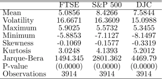
The empirical application is based on financial indexes, observed on a daily basis during the last 15 years. The datasets have been downloaded from Datastream. The series are the FTSE 100 index, the Standard & Poor’s 500 composite and the Dow Jones 65 composite (see Table 1). As before, letting St the observed price,

the returns are defined as 100×[logSt −logSt−1]. The descriptive statistics in

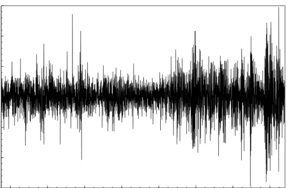
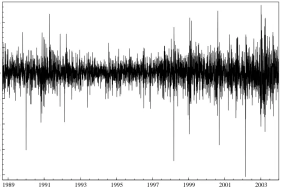
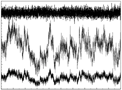
Table 2 report the per cent annualized means and volatilities. They are obtained by multiplying the sample mean and the sample standard error by 252 and √252 respectively. The annualized volatility for all the indexes lie between the 15 and the 17 percent. Furthermore, it is evident that all the series sensibly reject the hypothesis of normality. Daily returns are displayed in Figures 1-3.

All the calculations made in this paper are based on software written by using the Ox°c_{3.0 language of Doornik (2001).}

(17)

4.1 Posterior Analysis

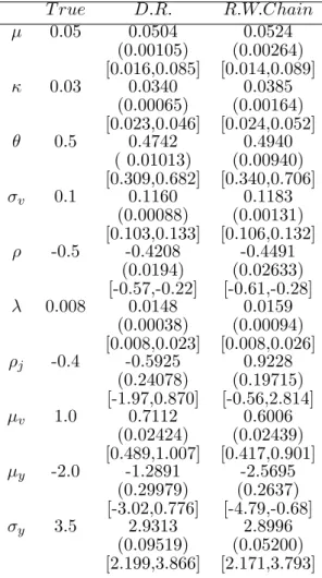
Inference has been performed for the general model described by eq. (18)-(19). Of course, the important particular cases such as the model proposed by Bates (Bates 1996) and the model introduced by Heston (Heston 1993) have been estimated. In order to check the fairness of the algorithm proposed, a simulated data set has been estimated. It is a time series of 2,000 observations generated by the contem-poraneous jumps stochastic volatility model. Results are reported in Table 3. In general the posterior means are close to the true values. Anyway it seems that the parameters related to the jump sizes are not accurately estimated. This is probably due to the fact that a jump is a rare event and then the number of observations affected by this happening are not many in the entire time series.

In order to control an eventual bad behaviour of the algorithm in some area of the support of the parameters, the chain generated has been perturbed by random and deterministic shocks. Some graphical analysis showed that after the shock, the chain return to its regular paths in few iterations.

Figure 4 evidences the decreasing number of rejections observed when using differ-ent proposals and the delayed rejection method. It is eviddiffer-ent that the number of rejections for the random walk chain and the independence chain are sensibly higher with respect to the delayed rejection. The estimate of the latent processes fit fairly well the ones generated. This is showed in Figures 5-6.

The analysis on real data is implemented through MCMC. The chain has been run for 50,000 iterations with a burn-in of 10,000. This seems an appropriate choice for the models considered. The Monte Carlo standard error (MCSE) has been com-puted through the use of a kernel estimator to take into account the dependencies due to the Markov nature of the algorithm. Since draws from the posterior distri-butions are not independent, the reported MCSEs are an estimate of 2π times the spectral density matrix at frequency zero computed by standard time series method. In particular, the estimator is based on a VAR(1) prewhitening, than 2π times the spectral density matrix at frequency zero of VAR residuals is estimated by smoothing methods using the Parzen kernel and automatic bandwidth selection. Recolouring provides an estimate of 2π times the spectral density matrix at frequency zero of interest. Tables 4-6 report the posterior means, together with the Monte Carlo stan-dard error and and the 95% confidence intervals evaluated using the percentiles of the empirical posterior distribution.

From a computational point of view it is interesting to note how the Delayed Rejec-tion algorithm performs. The introducRejec-tion of the random walk steps sensibly reduce the autocorrelation induced by the Markov structure of the algorithm. The number of rejections is similar to the one observed for the simulated data and basically re-duce to the 5% using a Delayed Rejection based on 3 steps. Figures 7 and 9 show the improvement between the two methods analyzed. The effect is impressive and some empirical studies evidence that it is possible to obtain similar autocorrelations recording just one draw every four or five.

(18)

re-sults obtained for the stochastic volatility model, while the third and the fifth show the results for the models with jumps. For comparative purposes, results based on the random walk algorithm are showed in the fourth column. For the simple stochastic volatility model, the average annualized volatility is √252×θ. The es-timate of the quantity is 16.9, that is really close to the sample volatility 16.66, as evidenced in Table 2. The parameter κ is the mean reversion of the volatility equation and is 0.024 and basically represents the time the process come back to its expected value level. The leverage effect between processes is mild: this finding is slightly different with previous results stylized in literature (see for example Eraker et al. 2003), but on the other side the period of reference considered here is differ-ent. The variance of the volatility process is σ2

vVt and then the parameter σv, that

is 0.131, is important to asses the volatility of the volatility behaviour. If the first jump component is taken into account, the volatility decreases, and the same thing happens to the parameter σv. This is because the introduction of a jump

compo-nent explains part of the volatility that in the previous model has been described just by a diffusive process. The parameter λ is 0.02. This means that the model expects 5.3 jumps per year. The annualized spot volatility, i.e. p252(θ+µvλ)/κ

reduces to 16.1 percent and the annualized total volatility, i.e. the mean square error of the returns that take into account the jump component is 16.94 percent. This latter statistic is computed according to eq. (13) and eq. (16) of Section 2. In percentage terms, the average effect of the jump component on the total volatility is approximately the 8.8 percent. Finally the more general model is analyzed. The introduction of the second jump component sensibly increase the parameterκ and then the mean reversion phenomenon sensibly speeds up. The parameterλ halves. The general model expects just 2.8 jumps per year. The annualized spot volatility sensibly decreases with respect to the other models and is the 15.6 percent. On the other side the total volatility is the 16.2 percent and then the return jump increases it of about 7.4 percent. It is evident that there exists a reduction with respect to the SVJ model. This is due to the extra jump component that itself explains part of the volatility behavior of the complete model. In fact, the contribution of the jump on volatilities shift√Vt−to

√

Vt−+Hv. The effect is mild with respect to the findings

showed in Eraker et al. (2003) and in this work is approximately the 3.3 percent. These differences can be explained by the different time interval considered for the empirical analysis. Eraker et al. (2003) in fact include October, the 19-th 1987 in which a huge crash in the markets has been observed. It is really likely that the single observation heavily influence all the estimates. Figures 10 and 11 show the estimates of the latent processes for the various models. At a first sight they seem equal, but a more detailed analysis evidence the findings stressed by the statistics on the volatilities described before.

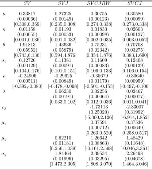
Results for S&P 500 are reported in Table 5. For this series, the mean reversion parameterκ increases sensibly by moving from the basic stochastic volatility model to the model with contemporaneous jumps. For the SV and the SVJ it is 0.011 while for the SVCJ is 0.026. At the same timeθ, that represents the average of the volatility process, decrease from 1.19 for the SV to 1.4 for SVJ and drop to 0.70 in the SVCJ. The spot annualized volatility for the Heston’s model is close to the 22 percent. In the Bates’ model this quantity diminish to the 19 percent. The total

(19)

volatility for the returns is about the 20.5 percent. This means that the jump effect explains about the 14 percent of the whole volatility. In the complete model the diffusive volatility drops to the 16 percent. The total volatility increases of just 1 point. Even in this case the average volatility jump’s size is negligible and is equal to 1.6 percent. It is interesting to note that for this data set the sensible change for λ. It moves from 0.06 to 0.02. The estimated volatilities are showed in Figure 12 while the probabilities of jump are showed in Figure 13.

Finally results for the Dow Jones index are reported in Table 6. The findings for this time series are similar to the results obtained for the others. The introduction of the jump process reduce the diffusive volatility component. As usual this is evidenced by the parameters θ and σv. As before the introduction of the jumps

slightly increases the mean reversionκ. This series anyway seems more regular than the others. The parameterλdoes not change much when the two models with jumps are chosen and the estimate is 0.003 for the Bates’ model and is 0.004. In general, for all the three models the volatility is low (6.5 percent) and it seems it is not affected by the jumps. The estimates of the latent processes are showed in Figures 14-15.

4.2 Model ranking

The contemporaneous jumps stochastic volatility model proposed in Duffie et al. (2000), say (M3,θ3) encompasses the model proposed in Bates (1996), i.e. (M2,θ2)

and the model proposed in Heston (1993), that is (M1,θ1). A standard practice

is to compute the Bayes factor in order to rank the various competing models. As stressed in Section 3.2 the ratio is defined as

The prior among models is uniform, i.e. p(Mi) =p(Mj) = 1/3,∀i, j. The details of

the procedure adopted here for the models considered has been showed in Section 3.2.1.

The estimates of the Bayes factors are reported in Tables 7-8. According to the thresholds defined in Kass & Raftery (1995), in general the complete model is strongly preferred to the others.

For the FTSE series, the ordering among the three models is remarkable. The model (M3,θ3) is strongly preferred to the others. Again, (M2,θ2) is better than

the simple stochastic volatility (M1,θ1). The logarithm of the Bayes factors are

always superior to 4 and then there is no uncertainty about the ranking.

For the S&P500, SVCJ is preferred to the SVJ, but the evidence is not so strong. In fact the log-Bayes factor is 1.56. Furthermore, the stochastic volatility with jump on the returns is systematically preferred to the plain stochastic volatility.

(20)

References

A¨ıt-Sahalia, Y. (2002), ‘Maximum Likelihood Estimation of Discretely Sampled Dif-fusions: a Closed-Form Approximation Approach’,Econometrica 70, 223–262. Bakshi, G., Cao, C. & Chen, Z. (1997), ‘Empirical Performance of Alternative

Op-tion Pricing Models’, Journal of Finance52, 2003–2049.

Bates, D. (1996), ‘Jumps and Stochastic Volatility: Exchange Rate Processes Im-plicit in Deutsche Mark Options’,Review of Financial Studies9, 69–107.

Bj¨ork, T. (1998), Arbitrage Theory in Continuous Time, Oxford University Press, New York.

Black, F. & Scholes, M. (1973), ‘The Pricing of Options and Corporate Liabilities’, Journal of Political Economy81, 637–654.

Carlin, B., Polson, N. & Stoffer, D. (1992), ‘A Monte Carlo Approach to Nonnor-mal and Nonlinear State-Space Modeling’, Journal of the American Statistical Association87, 493–500.

Carr, P. & Madan, D. (1999), Option Valuation Using the Fast Fourier Transform, Working paper, University of Maryland.

Chib, S. & Jeliazkov, I. (2001), ‘Marginal Likelihood from the Metropolis-Hastings Output’,Journal of the American Statistical Association 96, 270–281.

Chib, S., Nardari, F. & Shephard, N. (2002), ‘Markov Chain Monte Carlo Methods for Stochastic Volatility Models’,Journal of Econometrics108, 281–316.

Cyganowski, S. & Kloeden, P. (2000), MAPLE Schemes for Jump-Diffusion Stochas-tic Differential Equations, Technical report, Proc. 16th IMACS World Congress, Lausanne 2000, M. Deville and R. Owens eds.

Doornik, J. (2001), Ox: An Object-Oriented Matrix Programming Language, Tim-berlake Consultants Press.

Doucet, A., de Freitas, N. & Gordon, N. (2001),Sequential Monte Carlo Methods in Practice, Springer, New York.

Duffie, D., Filipovi´c, D. & Schachermayer, W. (2003), ‘Affine Processes and Appli-cations in Finance’,Annals of Applied Probability 13, 984–1053.

Duffie, D., Pan, J. & Singleton, K. (2000), ‘Trasform Anlysis and Asset Pricing for Affine Jump-Diffusions’,Econometrica 68, 1343–1376.

Durham, G. & Gallant, R. (2002), ‘Numerical Techniques for Maximum Likelihood Estimation of Continuous-Time Diffusion Processes (with comments)’,Journal of Business & Economic Statistics20, 297–337.

Elerian, O., Chib, S. & Shephard, N. (2001), ‘Likelihood Inference for Discretely Observed Non-Linear Diffusions’,Econometrica 69, 959–993.

(21)

Eraker, B. (2001), ‘MCMC Analysis of Diffusion Processes with Application to Fi-nance’, Journal of Business & Economic Statistics 19, 177–191.

Eraker, B., Johannes, M. & Polson, N. (2003), ‘The Impact of Jumps in Volatility and Returns’, Journal of Finance. (forthcoming).

Gallant, A. & Tauchen, G. (1996), ‘Which Moments to Match?’,Econometric Theory 12, 657–681.

G˚asemir, J. (2003), ‘On an Adaptive Version of the Metropolis-Hastings Algo-rithm with Independent Proposal Distribution’,Scandinavian Journal of Statistics 30, 159–163.

Ghysels, E., Harvey, A. & Renault, E. (1996), Stochastic Volatility, in C. Rao & G. Maddala, eds, ‘Statistical Methods in Finance’, North Holland, pp. 119–191. Gilks, W., Best, N. & Tan, K. (1995), ‘Adaptive Rejection Metropolis Sampling

within Gibbs Sampling’, Applied Statistics44, 455–472.

Gilks, W., Roberts, G. & Shau, S. (1998), ‘Adaptive Markov Chain Monte Carlo Through Regeneration’,Journal of the American Statistical Association93, 1045– 1054.

Gilks, W. & Wild, P. (1992), ‘Adaptive Rejection Sampling for Gibbs Sampling’, Applied Statististics 43, 337–348.

Glasserman, P. & Merener, N. (2001), Convergence of a Discretization Scheme for Jump-Diffusion Processes with State-Dependent Intensities, Working paper, Columbia University.

Gourieroux, C., Monfort, A. & Ranault, E. (1993), ‘Indirect Inference’, Journal of Applied Econometrics 85, 85–118.

Green, P. (1995), ‘Reversible Jump Markov Chain Monte Carlo Computation and Bayesian Model Determination’, Biometrika82, 711–732.

Han, C. & Carlin, B. (2001), ‘MCMC Methods for Computing Bayes Factors: A Comparative Review’, Journal of the American Statistical Association96, 1122– 1132.

Heston, S. (1993), ‘A Closed-Form Solution of Options with Stochastic Volatility with Applications to Bond and Currency Options’, Review of Financial Studies 6, 327–343.

Hull, J. & White, A. (1987), ‘The Pricing of Options on Assets with Stochastic Volatilities’, Journal of Finance42, 281–300.

Jacquier, E., Polson, N. & Rossi, P. (1994), ‘Bayesian Analysis of Stochastic Volatil-ity Models (with discussion)’,Journal of Business & Economic Statistics12, 371– 417.

(22)

Jacquier, E., Polson, N. & Rossi, P. (1999), Stochastic Volatility: Univariate and Multivariate Extensions, Working Paper, Scientific Series 99s-26, CIRANO. Johannes, M., Polson, N. & Stroud, J. (2002), Nonlinear Filtering of Stochastic

Differential Equations with Jumps, Working paper, Wharton School, University of Pennsylvania.

Kass, R. & Raftery, A. (1995), ‘Bayes Factors’,Journal of the American Statistical Association90, 773–795.

Kim, S., Shephard, N. & Chib, S. (1998), ‘Stochastic Volatility: Likelihood Inference and Comparison with ARCH Models’,Review of Economic Studies 65, 361–393. Kloeden, P. & Platen, E. (1995),Numerical Solution to Stochastic Differential

Equa-tions, 2 edn, Springer-Verlag, New York.

Maskell, S. & Gordon, N. (2001), A Tutorial on Particle Filters for On-line Nonlinear/Non-Gaussian Bayesian Tracking, Working paper, QuinetiQ Ltd. Meng, X.-L. & Shilling, S. (2002), ‘Warp Bridge Sampling’, Journal of

Computa-tional & Graphical Statistics11, 552–586.

Meng, X.-L. & Wong, W. (1996), ‘Simulating Ratios of Normalising Constants Via a Simple Identity: a Theoretical Explaination’, Statistica Sinica6, 831–860. Mengersen, K. & Tweedie, R. (1996), ‘Rates of Convergence of the Hastings and

Metropolis Algorithms’,Annals of Statistics 24, 101–121.

Mira, A. (2002), On Metropolis-Hastings Algorithms with Delayed Rejections, Work-ing paper, Universit`a dell’Insubria, Varese.

Nicholls, G. & Mira, A. (2003), Bridge Estiamtion of the Probability Density at a Point, Technical report n. 7, University of Insubria, Varese, Italy. To appear in: Statistica Sinica.

Pan, J. (2002), ‘The Jump-Risk Premia Implicit in Options: Evidence from an Integrated Time-Series Study’,Journal of Financial Economics 63, 3–50.

Peskun, P. (1973), ‘Optimum Monte-Carlo Sampling using Markov Chains’, Biometrika60, 607–612.

Pitt, M. & Shephard, N. (1997), Filtering Via Simulation: Auxiliary Particle Filter, Working paper, Nuffield College.

Protter, P. (1990), Stochastic Integration and Differential Equations: a New Ap-proach, Springer-Verlag, Berlin.

Robert, C. & Casella, G. (1999),Monte Carlo Statistical Methods, Springer, Berlin. Robert, C. P. (2001),The Bayesian Choice, 2 edn, Springer-Verlag, New York.

(23)

Roberts, G., Gelman, A. & Gilks, W. (1997), ‘Weak Convergence and Optimal Scaling of Random Walk Metropolis Algorithms’, Annals of Applied Probability 7, 110–120.

Runggaldier, W. (2003), Jump Diffusion Models, in S. Rachev, ed., ‘Handbook of Heavy Tailed Distributions in Finance’, North Holland.

Scott, L. (1997), ‘Pricing Stock Options in a Jump-Diffusion Model with Stochastic Volatility and Interest Rates: Applications of Fourier Inversion Methods’, Math-ematical Finance7, 413–424.

Smith, A. & Gelfand, A. (1992), ‘Bayesian Statistics without Tears: A Sampling-Resampling Perspective’, American Statistician 46, 84–88.

Tanner, M. & Wong, W. (1987), ‘Calculation of Posterior Distribution by Data Augmentation’, Journal of the American Statistical Association82, 528–540. Taylor, S. (1994), ‘Modelling Stochastic Volatility: a Review and Comparative

Study’, Mathematical Finance 4, 183–204.

Tierney, L. (1994), ‘Markov Chain for Exploring Posterior Distributions (with dis-cussion)’,Annals of Statistics 22, 1701–1762.

Tierney, L. (1998), ‘A Note on Metropolis-Hastings Kernels for General State Spaces’, Annals of Applied Probability 8, 1–9.

Tierney, L. & Mira, A. (1999), ‘Some Adaptive Monte Carlo Methods for Bayesian Inference’, Statistics in Medicine18, 2507–2515.

(24)

A

Conditional Posterior Distributions.

We will give the expression of the conditional distribution obtained for the model. In general, to make the notation simpler, I writeat=yt−µ−HtyJt,bt=Vt−Vt−1−

κ(θ−V_t₋₁)−Hv

tJt and ωt=σv2(1−ρ2)Vt−1. yt is the log-return at time t derived

as log(St)−log(St−1). For details on conjugate families see Robert (2001).

The main problem, as widely stressed in previous sections is to simulate the volatil-ity process for which doesn’t exist a closed form for the conditional posterior. Its expression is p(Vt|rest)∝ 1 Vtexp ( − σv2a2t +b2t −2ρσvatbt 2ωt − σ2 va2t+1+b2t+1−2ρσvat+1bt+1 2ωt+1 ) (42)

The jump timeJtis a sequence of Bernoulli random variables. In order to calculate

the conditional posterior it is sufficient to evaluateP(Jt= 1|rest) andP(Jt= 0|rest)

in the following way,

Pc(1) =P(Jt= 1|rest)∝λexp n_σ2 va2t,1+b2t,1−2ρσvat,1bt,1 ω o (43) Pc(0) =P(Jt= 0|rest)∝(1−λ) exp n_σ2 va2t,0+b2t,0−2ρσvat,0bt,0 ω o (44) with at,i = at, Jt = i and bt,i = bt, Jt = i, i= 0,1. The conditional posterior is a

Bernoulli withP(0) =Pc(0)/(Pc(0) +Pc(1)).

It is very easy to sample from theξY _{sequence. After some calculation it is possible}

to obtain p(H_ty|Jt= 1, rest)∝ N Ã σ2_v(yt−µ)2−ρσvbt+ (µy+ρjHtv)ωt/σ2y)σy2 σ2 vσ2y+ωt , σ 2 yωt σ2 vσ2y+ωt ! (45)

Analogous algebra leads to

p(H_tV|Jt= 1, rest)∝ N Ã ft−ρσv(yt−µ−Hty)−ωt/µv+ρj(HtY −µy)ωt/σy2 σ2 vσy2+ωt , σ 2 yωt σ2 y +ρ2jωt ! (46)

whereft=Vt−Vt−1−k(θ−Vt−1). IfJt= 0 then the posterior conditional simplify

to the law ofH_ti, i=y, v.

Parameters involved in the diffusion’s drifts are easy to sample too. It is trivial to check thatµ,kandkθare proportional to Normal distributions. The prior used are respectivelyN(0,25), N(0,1) and N(0,1). θ is obtained as a ratio of the previous two extraction.

(25)

Correlation among Brownian errors is explained by the parameter ρ. We assume a prior Uniform in (−1,1). The conditional posterior is then

p(ρ|rest)∝ 1 (p1−ρ2₎nexp ½ −1 2 n X t=1 ³_σ2 va2t +b2t −2ρσvatbt ωt ´¾ I_[₋₁_,_1](ρ) (47)

The variance of the error term of the volatility process isσ2

v. The prior we chose is

U(0,1). p(σ_v2|rest)∝ 1 σn v exp ½ −1 2 ³ σ_v2 n X t=1 a2 t ωt + n X t=1 b2 t ωt −2ρσv n X t=1 btat ωt ´¾ I_[0_,_1](σv) (48)

The conditional posterior both forρandσ_v2seems too complicate to handle directly. For this reason I decided to use ARMS to simulate from them.

The intensity λis sampled from

p(λ|rest)∼Beta µ 2 + n X t=1 Jt,40 +n− n X t=1 Jt ¶ (49)

Forµv, given that the prior is anIG(α0, β0),α0 = 20, β0 = 10, after some calculation

it is possible to show thatp(µv|rest)∝IG(n+α0, z+β0) withz=

P

Hv_.

The parameterρj represent the correlation between jump sizes. The prior imposed

is N(0,4). It is easy to show that its conditional distribution is proportional to a Normal distribution p(ρj|rest)∝N(c/(b+ 1/4),1/(4b+ 1)) in which et=Hty−µy,

b= (Pn_t₌₁Hv2

t )/σy2 and c= (

P_n

t=1etHtv)/σ2y.

The variance of the conditional distribution of the return jump size isσ2

y. Imposing

an Inverse Gamma prior IG(α0 = 5, β0 = 20) leads to a conjugate posterior. The

conditional posterior is then an Inverse Gamma IG(α+n/2, β+z/2), and where z=Pn_t₌₁¡H_ty−µy−ρjHtv

¢₂

. Finallyµy is Normal with mean

P

mt(n/σy2+ 0.01)−1 and variance (n/σy2+ 0.01)−1

(26)

B

Results

Table 1: Indexes, daily series

Price Index Symbol Period

Financial Times Stock Exchange 100 FTSE 4/7/1988- 4/7/2003 Standard & Poor’s 500 Composite S&P500 4/7/1988- 4/7/2003 Dow Jones Composite 65 Stock Ave. DJC 4/7/1988- 4/7/2003

Table 2: Descriptive statistics for annualized Index returns FTSE S&P 500 DJC Mean 5.0856 8.4266 7.5844 Volatility 16.6671 16.3609 15.0988 Maximum 5.9025 5.5732 5.3455 Minimum -5.8853 -7.1127 -8.1497 Skewness -0.1069 -0.1577 -0.3319 Kurtosis 3.0248 4.1393 5.2012 Jarque-Bera 1494.345 2801.362 4469.79 P-value (0.0000) (0.0000) (0.0000) Observations 3914 3914 3914

(27)

1989 1991 1993 1995 1997 1999 2001 2003 −4 −2 0 2 4 6

Figure 1: FTSE Returns - July 5,1988 - July 4,2003

1989 1991 1993 1995 1997 1999 2001 2003 −6 −4 −2 0 2 4

(28)

1989 1991 1993 1995 1997 1999 2001 2003 −8 −6 −4 −2 0 2 4

(29)

Table 3: Simulated Data - The first column show results obtained withdelayed re-jection on 3 stages. The second one the results based on a Random Walk chain

T rue D.R. R.W.Chain µ 0.05 0.0504 0.0524 (0.00105) (0.00264) [0.016,0.085] [0.014,0.089] κ 0.03 0.0340 0.0385 (0.00065) (0.00164) [0.023,0.046] [0.024,0.052] θ 0.5 0.4742 0.4940 ( 0.01013) (0.00940) [0.309,0.682] [0.340,0.706] σv 0.1 0.1160 0.1183 (0.00088) (0.00131) [0.103,0.133] [0.106,0.132] ρ -0.5 -0.4208 -0.4491 (0.0194) (0.02633) [-0.57,-0.22] [-0.61,-0.28] λ 0.008 0.0148 0.0159 (0.00038) (0.00094) [0.008,0.023] [0.008,0.026] ρj -0.4 -0.5925 0.9228 (0.24078) (0.19715) [-1.97,0.870] [-0.56,2.814] µ_v 1.0 0.7112 0.6006 (0.02424) (0.02439) [0.489,1.007] [0.417,0.901] µy -2.0 -1.2891 -2.5695 (0.29979) (0.2637) [-3.02,0.776] [-4.79,-0.68] σy 3.5 2.9313 2.8996 (0.09519) (0.05200) [2.199,3.866] [2.171,3.793]

(30)

Figure 4: Simulated data - Estimated rejection rate for the algorithm used to infer the model. Dotted line: Independence chain (medium line); Dashed line: Random walk chain (upper line); Solid line: Delayed Rejection (lower line)

0 500 1000 1500 2000 2500 3000 3500 4000 4500 5000 100 200 300 400 500 600

(31)

Figure 5: Simulated data - True (a) and estimated volatility processes (b). 0 150 300 450 600 750 900 1050 1200 1350 1500 1650 1800 1950 1 2 3 4 (a) 0 150 300 450 600 750 900 1050 1200 1350 1500 1650 1800 1950 1 2 3 4 (b)

Figure 6: Simulated data - True (a) and estimated probability jump processes (b).

0 150 300 450 600 750 900 1050 1200 1350 1500 1650 1800 1950 0.5 1.0 (a) 0 150 300 450 600 750 900 1050 1200 1350 1500 1650 1800 1950 0.5 1.0 (b)