1
Scheduling distributed energy resources and smart buildings of a Microgrid via
multi-time scale and model predictive control method
Xiaolong Jin
1, Tao Jiang
2*, Yunfei Mu
1*, Chao Long
3, Xue Li
2, Hongjie Jia
1, Zening Li
2 1 Key Laboratory of Smart Grid of Ministry of Education, Tianjin University, Tianjin 300072, China 2 Department of Electrical Engineering, Northeast Electric Power University, Jilin, Jilin 132012, China 3 Institute of Energy, School of Engineering, Cardiff University, Cardiff CF24 3AA, UK*[email protected], [email protected]
Abstract: To schedule the distributed energy resources (DERs) and smart buildings of a Microgrid in an optimal way and consider the uncertainties associated to forecasting data, a two-stage scheduling framework is proposed in this paper. In stage I, a day-ahead dynamic optimal economic scheduling method is proposed to minimise the daily operating cost of the Microgrid. In stage II, a model predictive control based intra-hour adjustment method is proposed to reschedule the DERs and smart buildings to cope with the uncertainties. A virtual energy storage system is modelled and scheduled as a flexible unit using the inertia of building in both stages. The underlying electric network and the associated power flow and system operational constraints of the Microgrid are considered in the proposed scheduling method. Numerical studies demonstrate that the proposed method can reduce the daily operating cost in stage I and smooth the fluctuations of the electric tie-line power of the Microgrid caused by the day-ahead forecasting errors in stage II. Meanwhile, the fluctuations of the electric tie-line power with the MPC based strategy are better smoothed compared with the traditional open-loop and single-period based optimisation methods, which demonstrates better performance of the proposed scheduling method in a time-varying context.
NOMENCLATURE
Abbreviations:
HAVC Heating, ventilation, and air conditioning. VESS Virtual energy storage system.
BIM Buildings-integrated-Microgrid. DER Distributed energy resource. DG Distributed generator. PV Photovoltaic.
BEMS Energy management system of building. MEMS Energy management system of Microgrid. MPC Model predictive control.
Sets and indices:
J, j Set of indexes of the wall orientations of a building.
T, t Set of indexes of the scheduling time periods. DG, i Set of indexes of the controllable DGs. BD, m Set of indexes of the buildings. EC, n Set of indexes of the electric chillers.
Parameters and constants:
Cph, Cse Electricity purchasing/ selling prices ($/kWh).
Pel,m Electric load of building m (kW).
Pload Electric load of the Microgrid except the electric load of buildings (kW).
PPV, PWT Electric power generated by photovoltaic system and wind system (kW).
Uwall, Uwin Heat transfer coefficient of the wall/window of the building [W/(m2K)].
Fwall,j The area of the total wall surface at the jth wall orientation (m2).
Fwin,j The area of the total window surface at the jth wall orientation (m2); It is assumed that the total window surfaces are distributed in the south, west, north and east orientations of the walls in a building uniformly.
Tout Outdoor temperature (ºC).
τwin The glass transmission coefficient of the windows.
SC The shading coefficient of the windows. αw Absorbance coefficient of the external surface
of the wall.
Q̇in Internal heat gains from people, appliances and lighting (kW).
ρ, C, V The density (kg/m3), specific heat capacity [J/(kgºC)] and volume of the air (m3) in the building.
Rse, j The external surface heat resistance for convection and radiation of the external wall j (m2K/W).
IT, j The total solar radiation on the walls/ windows surface at the j-wall orientation (kW/m2). EEREC Energy efficiency ratio of the EC.
ρ Maintenance cost of the energy devices ($/kWh).
QEC The upper limit of the cooling power output of the EC (kW).
Tin, Tin The upper and lower limits of the indoor temperature set-points of the building (ºC).
Pgrid, Pgrid The upper and lower limits of electric power exchange with the utility grid of the building (kW).
Pbt, Pbt The upper and lower limits of charging/discharging power of the battery (kW).
PDG, PDG The upper and lower limits of power generation of DG (kW).
Ru, Rd Ramp-up/ramp-down rate of a controllable DG (kW/min).
Su, Sd Startup/shutdown rate of a controllable DG (kW/min).
UT, DT Minimum up/down time periods of a controllable DG (h).
a, b, c Fuel cost coefficients of the diesel engine. ηFC Efficiency of the fuel cell.
ηch, ηdis Charging/discharging efficiency of the battery.
2 SOC, δ The state of charge/self-discharge ratio of the
battery.
Variables:
Pgrid Electric power exchange with the utility grid (kW).
Pgas Natural gas consumption (kW).
PEC Electric power consumption by the EC (kW).
Ploss Power loss of the electric network (kW).
Q̇EC Cooling power generated by the EC (kW). Q̇wall Heat transfer through the external walls (kW). Q̇win Heat transfer across the windows (kW). Q̇sw Heat contribution due to the solar radiation on
the opaque surface of the external walls (kW). Q̇sg The whole solar radiation transmitted across the
windows (kW).
Q̇cl,building Cooling load of the Microgrid with VESS being scheduled (kW).
Q̇ ′cl,building Cooling load of the Microgrid without VESS being scheduled (kW).
Pbt Charging/discharging power of battery (kW).
PDG Power generation of DG (kW).
UDG Operation status of DG, where “1” represents ‘ON’-state and “0” represents ‘OFF’-state. U'DG, Startup status of DG, which is “1” for startup
and “0” for otherwise.
U''DG Shutdown status of DG, which is “1” for shutdown and “0” for otherwise.
Ton, Toff Number of successive ON/OFF time periods of DG (h).
Tin Indoor temperature (ºC).
1. Introduction
1.1. Background
The recent years experienced a rapid increase of power consumption in buildings worldwide due to the rapid process of urbanization of the world’s population [1]. It has been shown that global use of electricity in buildings grew on average by 2.5% per year since 2010, and it increased by nearly 6% per year [2]. According to the International Energy Agency, buildings’ share of the worldwide energy usage is approximately 40%, with almost half of it being used in their heating, ventilation and air conditioning (HVAC) systems [3]. After more than 30 years of rapid economic development, China has become a large CO2 emitter with its increasing energy consumption [4]. The building sector currently accounts for 27.6% of the total energy use and it is estimated to reach 35% by 2020 in China [5]. Therefore, issues on energy consumption reduction of buildings will become more prominent in China.
1.2. Motivation
Power consumption related to thermal appliance operation for heating/cooling purposes in a building, such as HVAC and electric chiller, represents a very high portion in load demand. For most of the applications of heating/cooling devices, it is only required to control the temperature in a suitable zone without disturbing the temperature comfort level [6]. This provides an opportunity to effectively reduce the energy usage/cost and the peak demand of buildings by scheduling the heating/cooling devices in an optimal way. Hence in principle, buildings have the potential to become a huge source of flexibility to reduce the load demand, facilitate integration of intermittent renewable generation and provide ancillary services to power systems [6].
Microgrids offer an opportunity and a desirable infrastructure to schedule smart buildings of a community in an optimal way by utilizing advanced energy management technologies and intelligent communication technologies [7]. It leads to the concept of Buildings-integrated-Microgrid (BIM). Several benefits and opportunities can be achieved by applying the Microgrid energy management on the BIM system: 1) Buildings can enjoy energy/cost savings [8]; 2) Intermittent renewable generation can be more efficiently integrated [9]; 3) Distributed energy resources (DERs) at building side, such as controllable distributed generators (DG), storage devices and electric vehicles, are more efficiently managed [10]; 4) Power imbalance of the Microgrid can be balanced by optimal scheduling the DER and smart buildings without being charged for reserve service from the utility grid [11]. Therefore, Microgrid energy management in buildings is attracting more and more attentions in recent years. The PV and wind based DGs are uncontrollable due to their characteristics of randomness and intermittent. In this context, the PV and wind based DGs are not included in the investigated DERs in this paper.
1.3. Related work and research gaps
Studies have been carried out to investigate the energy management methods for a BIM. Optimal day-ahead scheduling methods were investigated for a BIM in [9]-[14] achieving different operational objectives, such as operating cost reduction and pollutants emission reduction. The main idea is that optimisation technologies are used to decide day-ahead optimal schedules of the BIM based on day-day-ahead forecasting data, day-ahead electricity prices and technical information of energy devices of the BIM. However, the inherent uncertainties of the day-ahead forecasting data are not considered, which leads to a discrepancy between the power really exchanged with the utility grid and the planned one. To further consider the uncertainties associated to the day-ahead forecasting data, stochastic day-ahead scheduling methods were proposed in [15] and [16] by using scenario-based method and scenarios reduction techniques. Nevertheless, the stochastic optimal scheduling methods assume the day-ahead forecasting data follows certain probability density functions. The probability density functions require sufficient historical data, which limits the application of the stochastic method [17]. Meanwhile, the probability density functions may be inappropriate to describe the uncertainties in practical applications [18]. Robust day-ahead scheduling method is another way to consider the uncertainties for scheduling a BIM, as proposed in [19][20]. However, concerns of its practical application are the conservativeness, as the robust optimal scheduling method is based on the worst-case analysis [21]. The above optimal day-ahead scheduling methods have made good contributions to the optimisation of a BIM. However, since the operational time scales of a BIM system are different between the day-ahead stage and actual operational stage, the day-ahead methods with one single time scale are difficult to capture the temporal dependencies of the schedules of the DERs and smart buildings between the two stages. In this context, the optimal schedules determined by the day-ahead methods leave questions on their feasibility and actual performances for practical applications on the BIM. Furthermore, although the uncertainties of the day-ahead forecasting data are considered at day-ahead scheduling stage, their dynamic random fluctuations are not considered at
3 actual operational stage, which still causes errors between the
schedules of two stages and further induces fluctuations of the electric tie-line power of the BIM. As stated in [22], balancing the errors and smoothing the fluctuations are important for the benefits of the utility grid and the BIM.
To cope with the above problems, multi-time scale and multi-stage scheduling methods for BIM system have gained much attentions recently. A multi-time scale and coordinated scheduling method for a multi-energy BIM was proposed in [22]. A two-stage robust scheduling method for a BIM system was proposed in [23] to minimize the operating cost. A multi-time scale stochastic scheduling method was proposed in [24] to schedule deferrable appliances and energy resources of a smart building in an optimal way considering the uncertainties of forecasting data. However, the flexibility of the building with heat inertia has not been fully explored in the above work. In [25], a two-stage hierarchical Microgrid energy management method in an office building by scheduling thermal mass of the building and plug-in electric vehicles was proposed. The daily operating cost can be reduced at the day-ahead stage and the fluctuations of the electric tie-line power can be smoothed to some extent at the intra-hour stage with the proposed method. Although the flexibility of the building was considered in [25], the optimal scheduling method used at actual operational stage was open-loop and single-period based in nature. In other words, the optimal schedules at actual operational stage are optimized using the single-period based optimisation strategy based on the operating status of the BIM and forecasting data at current operational period rather than the predictive operating status and forecasting data over a future time horizon [26]. In this case, concerns regarding the optimal adjustments of the controllable units of the BIM at the actual operational stage, such as insufficient adjustments, excessive adjustments and untimely adjustments, would arise [27]. This leads to bad control performance of the single-period optimisation strategy in a time-varying context with uncertainties associated to forecasting data.
Different to the open-loop and single-period strategy, model predictive control (MPC) based scheduling method leads to better control performance against uncertainties because of its capability to handle the future behaviour of the BIM system, demand and renewable generation forecasts and the constraints of the BIM. MPC computes a sequence of decision variable adjustments over a future time horizon iteratively based on an underlying optimisation model and forecasting data of uncertain variables [28]. In other words, MPC is a rolling process that runs the embedded optimisation model repeatedly with updated forecasts, which has better control performance in a time-varying context, as verified in [29]. Motivated by the attractive features of MPC method in time-varying context, an MPC-based scheduling strategy for the BIM is developed at the intra-hour adjustment stage in this paper. The intra-hour adjustment stage can smooth the fluctuations of the electric tie-line power of the BIM caused by the errors of the day-ahead forecasting data.
Furthermore, these existing approaches consider the aggregate supply-demand balance while omitting the underlying electric network, the associated power flow (e.g., Kirchhoffs laws), and system operational constraints (e.g., voltage tolerances). Consequently, such approaches may result in control decisions that violate the real-world constraints [30]. Therefore, this paper focuses on developing
an optimal scheduling method for a Microgrid via multi-time scale and model predictive control method. The power flow and system operational constraints of the electric network of the Microgrid is considered in the proposed scheduling method.
1.4. Contributions of this paper
To schedule the DERs and smart buildings of a Microgrid more efficiently and bridge the research gaps, a novel two-stage scheduling method for a BIM system via multi-time scale and MPC method is proposed in this paper. The main contributions are summarized as follows:
1) A novel two-stage method is proposed for scheduling DERs and smart buildings of a Microgrid by using multi-scale and MPC method. The proposed scheduling method consists of a day-ahead dynamic optimal economic scheduling stage and an intra-hour rolling adjustment stage. The framework takes care of two different objectives, i.e., reducing the daily operating cost and smoothing the fluctuations of the electric tie-line power, which benefits both the BIM and the utility grid.
2) The configuration of the energy management system of Microgrid (MEMS) and energy management systems of buildings (BEMSs) are presented and the interactions between the MEMS and BEMSs are also introduced. MEMS and BEMSs compute the hourly optimal schedules of DERs and smart buildings for daily operating cost reduction of the BIM based on the hourly day-ahead forecasting data at the first stage. Whereas at the second stage, the MEMS and BEMSs reschedule the DERs and the smart buildings to smooth the fluctuations of electric tie-line power of the BIM due to the errors of day-ahead forecasting data. The optimisation is done with information exchange between the two stages and the interactions between the MEMS and BEMSs.
3) A building is simplified to a lumped thermal mass and modelled as a simplified thermal storage system, namely the virtual energy storage system (VESS), which is scheduled as a flexible resource to fully explore the flexibility of the building with its thermal mass.
4) To improve the control performance in a time-varying context with uncertainties associated to forecasting data, the MPC based scheduling method is used at the intra-hour adjustment stage. By using the iterative rolling optimisation with finite horizon instead of the traditional open-loop and single-period based optimisation, the problems of the insufficient adjustments, excessive adjustments and untimely adjustments of the DERs and smart buildings at intra-hour stage can be solved.
5) Various practical constraints from the buildings and the DERs are considered in the proposed scheduling method. Moreover, a Microgrid is a low-voltage distribution network that is located down-stream of a distribution substation through a point of common coupling. Therefore, power flow and system operational constraints of the electric network of the Microgrid are also considered in the proposed scheduling model.
6) The proposed scheduling method provides a flexible energy management platform for BIM, which can be extended for optimal scheduling for other energy resources, such as electric vehicles. As a flexible resource, the integration of electric vehicles to the building is creating new opportunities for the Microgrid energy management. The electric vehicles integrated to the building can be modelled as
4 an aggregated DER under the Vehicle-to-Building (V2B)
concept [31]. Then, the EVs can be scheduled as another DER with the proposed scheduling method.
The structure of this paper is summarized as follows. In Section 2, the system description and the mathematical model of the BIM is presented. Section 3 presents a detailed description and the mathematical model of the proposed multi-time scale and model predictive control based scheduling method. Section 4 discusses the scheduling results of the BIM in both scheduling stages and demonstrates the effectiveness of the proposed method by carrying out several comparative scenarios. Finally, Section 5 concludes the whole paper.
2. Configuration and modelling of an BIM
2.1. Configuration of the BIM
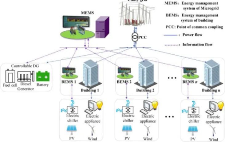
The physical configuration of an BIM is shown in Fig. 1, mainly including multiple smart buildings, DERs (i.e., controllable DGs and battery), the MEMS and BEMSs installed in each smart building. The energy systems of a smart building include an electric chiller for cooling purpose, the renewable generations and other electric appliance. The proposed optimal scheduling method is based on information exchange between the MEMS and the BEMSs thanks to the communication infrastructure of the BIM. The functions of the MEMS and BEMS are described as follows:
Fig. 1. Configuration of the BIM
MEMS: MEMS monitors the energy consumption of buildings and interacts with every BEMS to optimise their energy usage within the user’s comfort range. With the proposed scheduling method and the forecasting data from the BEMSs, optimal schedules of the DERs and the smart buildings are obtained and issued to the corresponding DG controllers and the BEMSs. The optimal schedules of the DERs include operational schedules at day-ahead stage, i.e., the unit commitment of the DGs and the charging/discharging schedules of the battery, and adjustment reschedules at intra-hour stage, i.e., the optimal adjustments of power outputs of the DGs and the charging/discharging power of the battery. The optimal schedules of each smart buildings at both stages are the optimised power consumption profiles of the electric chiller, which are used as control variables to fully explore the flexibility of the buildings.
BEMS: Forecasting data of solar radiation and outdoor temperature is obtained by BEMS from the weather station through the communication links. Meanwhile, the forecasting data of each building, i.e., electric power consumption of the electric appliance and internal heat gain,
are obtained by BEMSs. All the forecasting data from BEMSs are uploaded to the MEMS. With the optimised load profile of each building issued by the MEMS and thermal model of the building, the indoor temperature schedules for each building are calculated by the BEMS and issued to the indoor temperature controller.
Communication infrastructure: For the optimal scheduling method, a bidirectional communication infrastructure is required between the BEMSs and the MEMS, as shown in Fig. 1. Also, unidirectional communication links are required between the BEMSs and the market operator, BEMSs and local weather station, MEMS and the DG controllers.
The smart buildings investigated in this paper are assumed to be public buildings that are centrally managed by a single public authority. Since the public buildings have the common interest of reducing the overall operating cost of the BIM, a centralized scheduling method is used in this paper. Future research will develop a decentralized scheduling method for private buildings that aims to minimise their own energy consumption and costs.
2.2. Components modelling
2.2.1 Building model: Considering a summer cooling scenario, a building is modeled as a single isothermal air volume [32]. The mathematical relationship among the indoor temperature, cooling demand and outdoor temperature is formulated to investigate the thermal performance of a building by using the building thermal equilibrium equation, as shown in Eq. (1) [33].
ρ×C×V×dTin
dt = Q̇wall+Q̇win+Q̇in+Q̇sw+Q̇sg-Q̇EC (1)
(i) Q̇wall is calculated by summing the contribution of each wall of a building, as shown in Eq. (2). The roof of a building is accounted for as part of the external walls [34].
(ii) Q̇win is calculated by summing the contribution of each window of a building, as shown in Eq. (3). (iii) Q̇in is the internal heat gains (kW).
(iv) Q̇sw is calculated by summing the heat contribution due to solar radiation on each external wall (south, west, north and east orientations) according to the ISO 13790 [35], as shown in Eq. (4). Also, the external surface heat resistance for convection and radiation of the external wall j, Rse, j, is considered in Eq. (4). A typical method to calculate the Rse, j is given in [36], which takes both radiation and convection terms into account.
(v) Q̇sg is calculated according to Eq. (5). It is assumed that the total windows surfaces are distributed in the south, west, north and east orientations of the walls in a building uniformly [37].
(vi) Q̇EC is the cooling power generated by the cooling equipment (kW).
Q̇wall=
Σ
j∈JUwall×Fwall,j×(Tout-Tin) (2)
Q̇win=
Σ
j∈JUwin×Fwin,j×(Tout-Tin) (3)
Q̇sw=
Σ
j∈Jαw×Rse,j×Uwall×Fwall,j×IT,j (4)
Q̇sg=
Σ
5 IT, j is determined according to the method presented
in Duffie and Beckman [38], which is a commonly used method to calculate the total solar radiation on a tilted surface [39]. It can be calculated as sum of various type of solar radiation, i.e., beam, diffuse and reflected radiation, as shown in Eq. (6):
IT = Ib×Rb+Id×(1+ cos β2 )+I×ρg×(1- cos β2 ) (6)
where Ib, Id and I represent beam, diffuse and total radiation on horizontal surface respectively (kW/m2); ρ
g is the ground reflectance and is taken as 0.2 in the present study [39]; Rb is geometric factor which is defined as the ratio of beam radiation on a tilted surface to that on a horizontal surface, which is expressed as:
Rb = cos θcos θ
z (7)
where θ and θz are incidence and zenith angles.
The thermal mass of a building can provide inertia. Like other technologies to store energy, this inherent property can be used to store energy at peak periods and preheat or precool the building without any additional investment cost. Therefore, the model of VESS is developed considering this inherent property of a building. The basic idea of the VESS is that the cooling demand of the building can be adjusted in the energy management process without disturbing the temperature comfort level due to the thermal mass of the building. Therefore, the cooling energy generated by the electric chiller is stored in the building when the electricity price is low, i.e., the electric chiller is started in advance or the power consumption of the electric chiller is increased. In that case, the VESS is charged seen from the Microgrid, i.e., Q'̇cl,building < Q̇cl,building. In the same way, the cooling energy generated by the electric chiller is discharged in the building when the electricity price is high, i.e., the electric chiller is shut down in advance or the power consumption of the electric chiller is decreased. In that case, the VESS is discharged seen from the Microgrid, i.e., Q'̇cl,building>
Q̇cl,building. The charging/discharging power of the VESS, as shown in Eq. (8), is obtained following Eq. (1). The indoor temperature comfort zone and temperature set-point are considered in the model of VESS to maintain the customer comfort level.
Q̇VESS,t=Q̇'cl,building,t-Q̇cl,building,t (8) 2.2.2 Mathematical models of DER:
1) Diesel engine
For diesel engine, the fuel cost depends on the power generation and fuel cost coefficients, which is shown in Eq. (9). 2 , , ,
(
)
fuel DE t DE t DE tf
P
aP
bP
c
(9) 2) Fuel cellFor fuel cell, the fuel cost depends on the power generation and efficiency ηFC, which is shown in Eq. (10).
( ) /
FC,t
fuel gas gas gas FC
f P C P C PFC t,t η (10)
3) Electric chiller
The electricity consumption of the electric chiller is determined by the cooling demand and the coefficient of performance, as shown in Eq. (11).
QEC, t=PEC, t×EEREC (11)
4) Battery
The state of charge (SOC) of the battery refers to the ratio of the residual energy to the rated energy. The SOC at dispatch time interval t is described in Eq. (12).
1 , , 1 , , 1- / 0 / 1- 0 ch bt t bt t bt t t t btt dis bt bt t SOC P t P SOC S CAP CAP OC P t P (12)3. The multi-time scale and model predictive control based scheduling method
3.1. Framework of the scheduling method
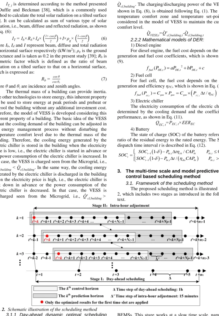
The proposed scheduling method is illustrated in Fig. 2, which includes two stages as introduced in the following text.
Fig. 2. Schematic illustration of the scheduling method 3.1.1 Day-ahead dynamic optimal scheduling stage: With the hourly electric load demand, outdoor temperature, solar radiation and the renewable generation forecasting values, the hourly schedules at day-ahead stage over the n1 time slots are obtained by the MEMS and the
BEMSs. This stage works at a slow time scale, namely ∆t. The hourly schedules include optimal schedules of the smart buildings (i.e., the optimized power consumption profiles of the electric chiller and the indoor temperature schedules), optimal schedules of the DREs (i.e., unit commitment of the
6 DGs and the charging/discharging schedules of the battery)
and day-ahead set-points of electric tie-line power.
3.1.2 Intra-hour rolling adjustment stage:Based on the day-ahead schedules, computed at the beginning of each scheduling day, a reference profile of the power exchange with the utility grid for the full day ahead is agreed with the utility grid and should be followed to avoid penalties and additional cost. Due to the forecasting errors of the day-ahead forecasting data, there are errors between the schedules of the BIM at day-ahead stage and intra-hour stage. This induces fluctuations of the electric tie-line power of the BIM. Therefore, an MPC based two-layer intra-hour adjustment stage is conducted to smooth the fluctuations of the electric tie-line power. Faster-time scale is set in this stage with a shorter time step ∆t'. As shown in Fig. 2, ∆t is further divided into four steps with an interval of ∆t'. The whole scheduling time-line at intra-hour stage is divided into n2 time slots and each time slot is allocated with 15 minutes.
The MPC based intra-hour rolling adjustment approach works as follows: At current time slot t'=k & k=1, the BEMSs and MEMS get the current forecasting data over the time horizon from k to k+Np-1 (i.e., the kth prediction horizon). The MEMS then solves a forward-looking optimisation problem to minimise the errors between the tie-line power at day-ahead stage and intra-hour stage over the Nc-slot time horizon (i.e., the kth control horizon). The optimised results are a sequence of adjustments of power output of the DGs, charging/discharging power of the battery and the power consumption of the electric chillers. Only the optimised results for the first-time slot at t', as highlighted in red in Fig. 2, are applied on the MEMS and issued to the corresponding DG controllers and the BEMSs. The unit commitment of the DGs and the charging/discharging status of the battery at intra-hour stage are kept the same with that at day-ahead stage. Then at next time slot t'=k & k= 2, the BEMSs and MEMS get updated forecasting data for the next Np time slots and the forward-looking optimisation problem
over the next control horizon again is solved again. And the optimized results for the first-time slot are applied as the optimal adjustments for current time slot. The time horizon moves forward by one-time slot for the new forward-looking optimisation until all the control schedules are determined during the whole time-line.
The current state of the BIM at each time slot is used as the initial set points of the MPC at each time slot in this paper, which is a commonly used method to determine the initial set points of the MPC [40]. The current state of the BIM is determined as follows: At each time slot (i.e., t'=k & k≠1), the current state of the BIM is updated according to the prediction model of the BIM (as formulated in Section 3.3.1) and the information of state-space of the BIM at previous time slot (i.e., t'=k-1). At the first time slot (i.e., t'=k & k=1), the current state of the BIM cannot obtained according to the prediction model of the BIM due to lack of the information of state-space of the BIM at previous time slot. Therefore, the day-ahead scheduling results at the first time slot of the day-ahead stage is used as the initial set points for MPC at the first time slot of the intra-hour stage.
3.2. Formulation of the scheduling method: Stage I
With the hourly electric load demand, outdoor temperature, solar radiation and the renewable generation
forecasting values, the hourly schedules of the day-ahead stage over the horizon T = {t=1, t=2, …, t=n1} are obtained by using an optimal dynamic scheduling program. The optimisation problem of stage I is formulated as follows.
3.2.1 Objective function: The objective function depicted in Eq. (13) is to minimise the total daily operating cost for the BIM.
, , , , , , , , , , , , , , , , , , , min + 2 2 t T fuel DG i t DG i DG i t ph t se t ph t se t gr su id t grid t WT t PV t bt t EC n t n i DG i t i DG WT PV bt EC EC C f P P U C C C P P P P P P
(13)The first term in Eq. (13) represents the cost for electricity purchase from the utility grid; The second term represents the fuel costs depicted by fuel cost function ffuel ( ), maintenance costs and the startup costs of all the controllable DGs; the third term is the maintenance costs of other devices of the BIM.
3.2.2 Constraints:
(1) Constraints of the Microgrid Electrical power balance:
grid,t DG,i,t el,m,t
i DG m BD load,t los dh WT,t PV,t bt,t EC,n,t s,t n EC P + + + P -P P P P - P = 0 t P P T
(14) Constraint of electric power exchange ,
grid,t dh
grid Pgrid t T
P P (15)
Power flow equations:
, , e e br e-bus e e br e-bus f t,ij i j ij ij f N j N f t,ij i j ij ij f N j N P - P V ,V ,Y ,θ = 0 t T Q - Q V ,V ,Y ,θ = 0 t T
t i t i (16)where Pt,i and Qt,i are the net injected active and reactive powers at the ith electric bus at time t.
Constraint of electric network
min max min max min max a i b i c i V V V V V V V V V (17) , ,max e e f f t ij ij
i
i
(18) -1
loop br e busN
N
N
(19)Eq. (16) is the electric power flow equation; Eq. (17) is the three-phase bus voltage constraint of the electric distribution network; Eq. (18) is the current constraint of the electric feeder; Eq. (19) is established to guarantee that the electric network has a radial structure.
(2) Constraints of the DERs Constraint of DGs
In the dynamic scheduling model, the constraints from the controllable DGs are introduced to consider the inherent link among the scheduling time intervals. For each controllable DG, the power generation is constrained by the upper and lower power output limits; The power generations between two successive dispatch time intervals are
7 constrained by ramp-up (ramp-down) rates as well as startup
(shutdown) rates, as shown in Eq. (20):
, , , , , , , , , , , , , , 1 , , -1 , , , , 1 , , , , , , , , , , , , 1 , , , , 1 , , , , , , = max 0, = max 0, DG i t DG i t DG i t DG i t DG i t DG i t DG i t DG i t DG i t DG i t DG i t DG i t DG i t DG i t DG i t DG i t DG i t DG i t DG i t u i u i d i d i P U P P U P P R tU S tU P P R tU S tU U U U U U U i DG , t T (20)The controllable DGs are also constrained by the minimum up and down time limits, as shown in Eq. (21).
, , , , 1 , , 1 , , , , -, DG i t DG i t DG i t DG i t on i t i off i t i T UT U U T DT U U i DG t T (21) Constraint of the battery
For the battery, the charging/discharging power and the SOC are constrained by the upper and lower limits shown in Eqs. (22) ~ (24); For the energy balance, the stored energy inside the battery is set the same as the initial stored energy, as shown in Eq. (25). ,
,
bt t bt btP
P
P
t T
(22),
tSOC
SOC
SOC
t T
(23) , bt t t bt E SOC CAP (24) ,0
t t t T bP
(25) Constraint of the electric chiller
0
Q
EC,t
Q
EC,
t T
(26) (3) Constraints of the buildings Cooling demand balance
Q̇EC,t=EEREC×PEC,t=Q̇cl,building,t, ∀t∈T (27)
Building thermal equilibrium equation ∆t[Q̇wall, t+Q̇win, t+Q̇sw, t+Q̇sg, t+Q̇in, t-Q̇EC, t]-ρCV(Tin, t+1
-Tin, t)=0, ∀t∈T (28)
Indoor temperature set-point constraint
, ,
in in t in t
T T T T (29)
3.3. Formulation of the scheduling method: Stage II
The MPC strategy with operational constraints is proposed to reschedule the smart buildings and DERs at intra-hour stage. The BEMSs and the local controllers of the DERs not only have to consider local information, but also exchange the state information with the MEMS, as introduced in Section 2.1. Therefore, the prediction model of the BIM is developed to inform the MEMS, BEMSs and DER controllers for rescheduling of the smart buildings and DERs. Then, the rolling optimisation problem is formulated and the implementation of the MPC based rescheduling method is introduced.
3.3.1 Prediction model:
(1) Prediction model of the Microgrid
According to the above system dynamics shown in Eqs. (1), (12) and (20), constraints of the Microgrid, DERs and smart buildings, as introduced in Section 3.2.2, the prediction model of the BIM is formulated using state-space, as shown in Eq. (30). The state of the Microgrid can be predicted by the iteration for the state-space model repeatedly with the updated forecasting data.
( 1) ( ) ( ) ( ) ( ) ( ) t A t B t C t t D t x x u r y x (30) where T ( )t Pgrid( ),t DG( ),t P tbt( ), SOC t( ), EC( )t x P P (31)
T ( )t Δ DG( ),t P tbt( ), Δ EC( )t u P P (32)
T ( )t PPV( ),t PWT( ),t Δ el( )t r P (33) ( )t Pgrid( )t y (34)Here x(t') is the state vector of the BIM at current time slot t', which consists of power exchange with the utility grid (Pgrid(t') ), vector of power output of controllable DGs (PDG(t')), charging/discharging power of the battery (Pbt(t'))
and its SOC value (SOC(t')), vector of power consumption of electric chillers (PEC(t')). u(t') is the control vector of the
BIM at current time slot t', which manages the increments of PDG(t'), Pbt(t') and PEC(t'), as shown in Eq. (32). The unit
commitment of the controllable DGs and the charging/discharging modes of the battery at intra-hour stage are kept the same with that at day-ahead stage. Therefore, they are not managed and controlled at intra-hour stage. r(t') is the input vector that influences the BIM at current time slot t', which consists of day-ahead forecasting errors of PV generation (∆PPV(t')), wind generation (∆PWT(t')) and electric loads of the buildings (∆Pel(t')). y(t') is the output of the prediction model of the Microgrid at current time slot t', which is the power exchange with the utility grid (Pgrid(t')). The matrices A, B, C and D are the relevant state-space matrices, as shown in Eqs. (35)-(38):
1 0 0 0 0 0 0 0 0 0 0 1 0 0 0 0 1 0 0 0 0 0 n m E A E φ δ (35) 1 1 1 0 0 0 1 0 0 0 0 0 n m E B E φ (36) 1 1 0 0 0 0 0 0 0 0 0 0 0 0 n E C (37)
1
0 0
D
0
0
(38)where En and Em are identity matrices; φ is the recurrence coefficient for SOC value calculation of the battery, as shown in Eq. (39).
8 , , 0 0 ch bt bt t bt t dis bt tη CAP t η P CAP P φ (39)
According to the model in Eq. (30), the predicted output of the Microgrid at time slot t'+p, can be calculated by the iteration based on the state at time slot t', as shown in Eq. (40):
1 1 ( | ) ( | ) ,..., 1| 1| p p p t p t D t p t D A x t A B u t A C r t B u t p t C r t p t y x (40)Then, the predicted output of the Microgrid over the kth prediction horizon can be formulated by the augmented vector, as shown in Eq. (41).
T 2 ( | ), ( 1| ),..., ( 1| ) , 1, 2,..., p k k k k k N k k n Y y y y (41)
(2) Prediction model of indoor temperatures of a building
The recurrence equation to predict the indoor temperature of a building can be obtained according to the building model, as shown in Eq. (42).
Tin(t'+1)-Tin(t')=
∆t(Q̇̂
wall+Q̇̂win+Q̇̂sw+Q̇̂sg+Q̇̂in-Q̇̂EC)
ρCV (42)
Q̇̂ is the updated value with the updated forecasting data of a building (λ(t')). λ(t') consists of forecasting errors of internal heat gain (∆Q̇in(t')), outdoor temperature (∆Tout(t'))
and solar radiation (∆IT(t')):
λ(t')=[∆Q̇in(t'),∆Tout(t'),∆IT(t')] (43) According to Eqs. (42) and (43), the indoor temperature of a building can be predicted by the iteration for the recurrence equation repeatedly with the updated forecasting data and the prior knowledge of state information of the Microgrid, as shown in Eq. (30) and (41).
3.3.2 Rolling optimisation: The objective is to keep the predicted output of the Microgrid, i.e., power exchange with the utility grid Pgrid(t'), close to the day-ahead schedules at each control horizon. The predicted output of the Microgrid over the kth control horizon is shown in Eq. (44).
T 2 ( | ), ( 1| ),..., ( 1| ) , 1, 2,..., c k k k k k N k k n Y y y y (44)The day-ahead schedules of the power exchange with the utility grid over the kth control horizon are generated in stage I and described as augmented vector, as shown in Eq. (45). T 2 ( | ), ( 1| ),..., ( 1| ) , 1, 2,..., dh dh dh
dh Pgrid k k Pgrid k k Pgrid k Nc k
k n Y (45) Then the optimisation problem for each control horizon can be formulated as:
T 1 2 min + ( ) . . (14) (29) c dh dh t k N bt bt t k f P t t s t
Y Y Y Y θ (46)where θbtis the penalty coefficient that limits the frequent charge and discharge operation of the battery. By adding the
penalty item on the objective function, the SOC values of the battery at stage II would follow that at stage I as close as possible.
3.3.3 Implementation process: In stage I, a day-ahead dynamic optimiser is designed at a slow time scale. The optimal day-ahead schedules are decided by running the dynamic optimisation problem with day-ahead forecasting data. In stage II, an intra-hour rescheduling method with faster time scale is proposed using MPC strategy. The mismatch between supply and demand due to forecasting errors is compensated by rescheduling the DERs and the smart buildings. Furthermore, a two-layer framework is specifically designed to coordinate and manage the MEMS, BEMSs and DG controllers effectively in stage II. Following the details introduced in Sections 3.2 and 3.3, the proposed scheduling method for the BIM can be realized by Algorithm 1 and its flowchart is shown in Fig. 3.
Algorithm 1 The multi-time scale and model predictive control based scheduling method.
Stage I: Day-ahead dynamic optimisation
1: Set sample interval ∆t = 1 h; t = 1; run time n1 = 24.
2: Take day-ahead forecasting data over the whole scheduling day:
ℤt=[Pel(t)TTout(t)TIT(t)TQ̇in(t)
T
PWT(t)TPPV(t)T]
T
, t = 1, 2, …, n1. 3: Solve the dynamic optimisation problem in (13), subject to the
constraints (14)-(29).
4: Output the day-ahead schedules of the BIM.
Stage II: Intra-hour rescheduling optimisation
5: Set sample interval ∆t' = 0.25 h; prediction horizon Np∗∆t'= 4 h;
control horizon Nc∗∆t'= 4 h; k = 1; run time n2 = 96. 6: fork = 1 : n2do
7: Set current time t' = k. 8: The master level: MEMS
9: Take the updated forecasting data over the kth prediction horizon: ℤt'=[Pel(t')TTout(t')TIT(t')TQ̇in(t') T PWT(t')TPPV(t')T] T , t' = k, k+1, …, k+Np-1.
10: Predict the output of the Microgrid over the kth control horizon based on the prediction model of the Microgrid in (30). 11: Collect the operational parameters of buildings and
controllable DGs.
12: Solve the rescheduling optimisation problem in (46) for the kth control horizon, subject to the constraints (14)-(29).
13: Output the optimal schedules over the kth control horizon:
T( )t Δ DG( ),t P tbt( ), Δ EC( )t
u P P t' = k, k+1, …, k+Nc-1.
14: Apply the optimized schedules for the current time step t' = k on the MEMS and issue the results to BEMSs and DG controllers.
15: The client level: BEMS of each building
16: Obtain the adjustment command for the electric chiller ∆PEC(t') at current time step t' = k.
17: Obtain the indoor temperature set-points based on ∆PEC(t')
and the recurrence equation in (42).
18: Apply the indoor temperature set-points on the heating, ventilation and air-conditioning systems.
19: The client level: DG controllers
20: Obtain the adjustment command for the DGs∆PEC(t') and
battery∆Pbt(t') at current time step t' = k.
21: Apply the adjustment command on the DG controllers. 22: k ← k+1 and go to step 7.
9 Fig. 3. Flowchart of the scheduling method
3.3.4 Solution algorithm: In this paper, the optimal scheduling problem is solved by using a co-simulation platform, as shown in Fig. A1 of Appendix A. The co-simulation platform consists of three modules, i.e., formulation and modelling module in MATLAB, optimisation solver in IBM ILOG CPLEX [41] and power flow calculation in OpenDSS [42]. The formulation of the optimisation problem (i.e., the objective functions and the constraints) and the model of the BIM (i.e., the building model, models of DGs and the Microgrid model) are implemented in MATLAB; MATLAB routes the optimisation model to the solver – IBM ILOG CPLEX Optimizer to solve the optimal scheduling problem; OpenDSS gets the optimal control variables from MATLAB and runs the sequential power flow of the electric network over successive time intervals. Then, the power loss is calculated while satisfying the network constraints of the Microgrid in OpenDSS. The principal procedure is described by Algorithm 2. This similar iteration-based algorithm has been applied on the optimal scheduling of an active distribution network [43] and an integrated community energy system [44].
Algorithm 2 The implementation procedure of the optimisation. 1: Set iteration coefficient IC1 = IC2 = 1 and their maximum values
n1 and n2; initial value of power loss Ploss0 ; precision coefficient e;
adjustment constant ∆Pe.
2: forIC2 = 1 : n2do 3: forIC1 = 1 : n1do
4: Solve the optimisation problem in CPLEX with Ploss0 .
5: Run power flow in OpenDSS based on the optimal control variables u=[PDG, Pbt,-PEC], u≤u≤u generated by
CPLEX.
6: Check the feasibility of the optimal solution.
7: if the lower limits of Eq. (17) are not satisfied or Eq. (18) is not satisfied then
8: Update the lower limits of control variables:
u ← u+∆Pe.
9: IC1 ← IC1+1 and go to step 4.
10: elseif the upper limits of Eq. (17) are not satisfied then
11: Update the upper limits of control variables:
u ̅← u̅-∆Pe. 12: IC1 ← IC1+1 and go to step 4. 13: else 14: break 15: end if 16: end for
17: Calculate the power loss Plossin OpenDSS.
18: if the change of power loss∆Ploss>ethen
19: IC2 ← IC2+1 and go to step 4 with the updated Ploss.
20: else
21: break
22: end if
23: end for
4. Results and discussion
4.1. Case study
A BIM shown in Fig. A2 of Appendix A containing smart buildings and DERs is used to verify the proposed scheduling method. Diesel engine 1, diesel engine 2, fuel cell, PV & battery and wind generator are connected to electric buses 680, 632, 633, 692 and 645 (B-phase), respectively. Four smart buildings are connected to electric buses 670, 671, 634 and 675, respectively. Day-ahead forecasting values of the outdoor temperature, solar radiations on horizontal surface, electric loads and internal heat gains of the four buildings, and renewable generations are shown in Figs. A3 - A5 of Appendix A. The capacity of the installed PV and wind based DGs are set to be 300 kW and 500 kW respectively. All day-ahead forecasting data are collected from [9]. The corresponding incident solar radiation on the walls/windows surface at south, west, north and east orientations are calculated based on the method presented by Duffie and Beckman, as shown in Fig. A3 of Appendix A. The electricity purchasing prices are shown in Fig. A6 of Appendix A, and the price for selling electricity back to the utility grid is set to be 0.8 times the price for purchasing electricity [10]. The short-term forecasting data over the prediction horizon at intra-hour stage need forecasting techniques, which are beyond the scope of this paper. Instead, we assume that the forecasting errors of all the data at intra-hour stage follows the uniform distribution [45]-[46], as shown in Eq. (47):
max max max max ( ) ( ) [1 ( )] ( ) ( ) [1 ( )] ( ) ( ) [1 ( )] ( ) ( ) [1 ( )] WT WT WT PV PV PV el el el out out t P t P t E R t P t P t E R t P t P t E R t T t T t E R t (47) where max WT E , max PV E , max el E and max t
E are the threshold values of the forecasting errors under different uncertainty levels, and their values are listed in Tab. B1 of Appendix B; R(t) is a random value that follows the uniform distribution: R(t)~U(-1,1). In this study, the uncertainty level is considered as Level 1.
The building studied in this paper is represented by a parallelepiped with a squared floor. The thermal parameters and the occupied hours of the buildings are given in Tab. B2 of Appendix B [9]. The values of the parameters of the air mass density and air specific heat ratio C are set to be 1.2kg/m3 and 1000J/(kgºC) respectively. The acceptable indoor temperature set-point range for human occupancy in a building varies under different operational scenarios. In this study, the indoor temperature set-point during occupied hours is set to be 22.5 ºC without VESS being dispatched. The indoor temperature set-point range during occupied hours is set to be from 19 ºC to 26 ºC with VESS being dispatched. It is worth noting that the electric chillers of the buildings are
10 switched off during unoccupied hours for cost saving. In this
context, the indoor temperatures are not optimised and no specific indoor temperature set-point range is assigned by the BEMSs during the unoccupied hours. The technical and economic parameters of the DERs are shown in Tabs. B3-B4 of Appendix B. The other operational parameters of the DERs are shown in Tab. B5 of Appendix B. The fuel cost coefficients of the diesel engine are set as: a=44 ($/h/MW2), b=65.34 ($/h/MW) and c=1.1825 ($/h). The natural gas price is 42.5$/MWh. All the parameters regarding the DERs are collected from Refs. [47]-[51].
4.2. Day-ahead scheduling results
The day-ahead schedules of the DERs are shown in Fig. 4. The results show that all the controllable DGs are committed and dispatched at their maximum capacities during high electricity purchasing price periods (i.e., 11:00– 12:00 & 14:00–18:00). They are switched off or the power generations are reduced for cost savings during low electricity purchasing price periods (i.e., 01:00–10:00 & 19:00–23:00). However, due to the constraint of electric power exchange, as shown in Eq. (15), required electric power cannot be imported from the utility grid at 08:00–10:00. Therefore, the fuel cell is committed and scheduled at 08:00– 10:00 to cover the power shortage without VESSs’ participation in day-ahead scheduling, as shown in Fig. 4(a)
1. However, the cooling demands of the buildings are adjusted
to reduce the power consumptions of the electric chillers considering VESSs’ participation, which results in no power shortage at 08:00–10:00. Therefore, unit commitment of the DGs is not needed at 08:00–10:00 and more cost savings are achieved. The PV and wind based DGs are uncontrollable DGs. In this context, their power outputs are not optimised and scheduled by the MEMS. Therefore, the schedules of the PV and wind based DGs are not presented in Fig. 4.
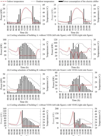
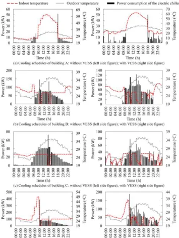
The day-ahead cooling schedules of the buildings are shown in Fig. 5. We can observe that the indoor temperatures are adjusted within the indoor temperature comfort range (19 ºC - 26 ºC) during the occupied hours by introducing VESS to the day-ahead scheduling stage. The indoor temperatures are kept at the set-points (22.5 ºC) during the occupied hours without considering VESSs’ participation. In this case, the daily operating cost of the BIM is reduced from $2128.9 to $2080.7, which is reduced by 2.3%. It can be concluded that the VESSs’ participation in day-ahead scheduling can reduce the daily operating cost of the BIM with limited modifications on the Microgrid management system. The day-ahead schedules of VESSs are shown in Fig. A7 of Appendix A. More details regarding the schedules of VESSs and their relationship with electricity purchasing prices are referred to Ref. [9] due to the limited space.
1 Only the fuel cell is scheduled at 08:00–10:00 because of its low-cost coefficient compared with the diesel engine.
Fig. 4. Day-ahead schedules of the DERs
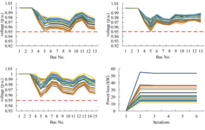
Fig. 5. Day-ahead cooling schedules of the buildings The three-phase voltages during one scheduling day are shown in Fig. 6 (a)-(c). It can be observed that the voltages of the network can satisfy the voltage limits (as shown in Eq.
11 (17)) using the proposed solution algorithm. The hourly
power losses of the network at each iteration are shown in Fig. 6(d). Initially, the power losses are assumed to be zero. After 5 iterations, the power losses converge to the steady states and the optimal day-ahead schedules of the BIM are found.
Fig. 6. Voltages and power losses of the network with VESSs’ participation
4.3. Intra-hour adjustment results
The day-ahead programming (DA-P) strategy used in [9] and single-period based strategy used in [25] are employed to compare with the MPC based strategy developed in this paper. Then the effectiveness of the proposed MPC based energy management method in the intra-hour stage is further verified.
DA-P strategy [9]: The DERs and VESSs are not rescheduled under the DA-P strategy in the intra-hour stage. Therefore, the errors between the schedules of day-ahead stage and intra-hour stage caused by day-ahead forecasting errors would be balanced by the utility grid.
Single-period based strategy [25]: The DERs and VESSs are rescheduled to cope with the day-ahead forecasting errors in the intra-hour stage. However, the rescheduled results of the DERs and VESSs are optimised based on the operating status of the BIM and forecasting data at current operational period rather than the predictive operating status and forecasting data over a future time horizon.
Different from the DA-P strategy and the single-period based strategy, the MPC based strategy reschedule the DERs and VESSs based on the predictive operating status and forecasting data over a future time horizon that runs the embedded optimisation model repeatedly with updated forecasts. The prediction horizon and control horizon are set to be 4 h [28] (i.e., Np=Nc=16) in the intra-hour adjustment stage in this paper.
Three comparative scenarios are carried out to verify the effectiveness of the proposed energy management method in the intra-hour stage. The DA-P strategy is named as Scenario I, single-period based strategy is named as Scenario II and the MPC based strategy is named as Scenario III.
Scenario I (DA-P strategy): Dispatch the BIM using day-ahead programming (DA-P) method [9]. Mismatches between the energy demand and supply caused by day-ahead forecasting errors are balanced by the utility grid, without rescheduling the DERs and VESSs.
Scenario II (Single-period based strategy): Reschedule the DERs and VESSs to cope with the day-ahead forecasting errors in the intra-hour adjustment stage using traditional single-period based optimisation strategy [25].
Scenario III (MPC based strategy): Reschedule the DERs and VESSs to cope with the day-ahead forecasting errors in the intra-hour adjustment stage using MPC based optimisation strategy.
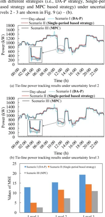
The electric tie-line powers of the BIM in the comparative scenarios are shown in Fig. 7 (a). Since all the mismatches between the energy demand and supply are balanced by electric power from the utility grid under the DA-P method in Scenario I, all the forecasting errors are mainly reflected in the electric tie-line power. The fluctuations of the electric tie-line power can be smoothed by rescheduling the DERs and VESSs in Scenario I and Scenario II.
Fig. 7. Intra-hour rescheduling results under uncertainty level 1