Spline-Based Image Registration
Richard Szeliski and James Coughlan
Digital Equipment Corporation Cambridge Research Lab
Digital Equipment Corporation has four research facilities: the Systems Research Center and the Western Research Laboratory, both in Palo Alto, California; the Paris Research Laboratory, in Paris; and the Cambridge Research Laboratory, in Cambridge, Massachusetts.
The Cambridge laboratory became operational in 1988 and is located at One Kendall Square, near MIT. CRL engages in computing research to extend the state of the computing art in areas likely to be important to Digital and its customers in future years. CRL’s main focus is applications technology; that is, the creation of knowledge and tools useful for the preparation of important classes of applications.
CRL Technical Reports can be ordered by electronic mail. To receive instructions, send a mes-sage to one of the following addresses, with the word help in the Subject line:
On Digital’s EASYnet: CRL::TECHREPORTS On the Internet: [email protected]
This work may not be copied or reproduced for any commercial purpose. Permission to copy without payment is granted for non-profit educational and research purposes provided all such copies include a notice that such copy-ing is by permission of the Cambridge Research Lab of Digital Equipment Corporation, an acknowledgment of the authors to the work, and all applicable portions of the copyright notice.
The Digital logo is a trademark of Digital Equipment Corporation.
Cambridge Research Laboratory One Kendall Square
Cambridge, Massachusetts 02139
Spline-Based Image Registration
Richard Szeliski and James Coughlan
1Digital Equipment Corporation Cambridge Research Lab
CRL 94/1 April, 1994
Abstract
The problem of image registration subsumes a number of problems and techniques in multiframe image analysis, including the computation of optic flow (general pixel-based motion), stereo correspondence, structure from motion, and feature tracking. We present a new registration algorithm based on spline representations of the displacement field which can be specialized to solve all of the above mentioned problems. In particular, we show how to compute local flow, global (parametric) flow, rigid flow resulting from camera egomotion, and multiframe versions of the above problems. Using a spline-based description of the flow removes the need for overlapping correlation windows, and produces an explicit measure of the correlation between adjacent flow estimates. We demonstrate our algorithm on multiframe image registration and the recovery of 3D projective scene geometry. We also provide results on a number of standard motion sequences.
Keywords: motion analysis, multiframe image analysis, hierarchical image registration, optical flow, splines, global motion models, structure from motion, direct motion estimation.
c Digital Equipment Corporation 1994. All rights reserved.
Contents i
Contents
1 Introduction
: : : : : : : : : : : : : : : : : : : : : : : : : : : : : : : : : : : : : : :
12 Previous work
: : : : : : : : : : : : : : : : : : : : : : : : : : : : : : : : : : : : : :
23 General problem formulation
: : : : : : : : : : : : : : : : : : : : : : : : : : : : :
4 3.1 Spline-based motion model: : : : : : : : : : : : : : : : : : : : : : : : : : : :
5 4 Local (general) flow estimation: : : : : : : : : : : : : : : : : : : : : : : : : : : :
95 Global (planar) flow estimation
: : : : : : : : : : : : : : : : : : : : : : : : : : : :
126 Mixed global and local (rigid) flow estimation
: : : : : : : : : : : : : : : : : : : :
187 Multiframe flow estimation
: : : : : : : : : : : : : : : : : : : : : : : : : : : : : :
228 Experimental results
: : : : : : : : : : : : : : : : : : : : : : : : : : : : : : : : : :
239 Discussion
: : : : : : : : : : : : : : : : : : : : : : : : : : : : : : : : : : : : : : : :
30ii LIST OF TABLES
List of Figures
1 Displacement spline: the spline control verticesf(
u
ˆ jv
ˆj)gare shown as circles ()
and the pixel displacementsf(
u
iv
i)gare shown as pluses (+).
: : : : : : : : : :
62 Spline basis functions
: : : : : : : : : : : : : : : : : : : : : : : : : : : : : : :
7 3 Block diagram of spline-based image registration: : : : : : : : : : : : : : : : :
13 4 Example of general flow computation: : : : : : : : : : : : : : : : : : : : : : :
14 5 Block diagram of global motion estimation: : : : : : : : : : : : : : : : : : : :
16 6 Example of affine flow computation: translation: : : : : : : : : : : : : : : : : :
17 7 Example of affine flow computation: divergence (zoom): : : : : : : : : : : : :
17 8 Example of 2D projective motion estimation: : : : : : : : : : : : : : : : : : :
19 9 Example of 3D projective (rigid) motion estimation: : : : : : : : : : : : : : : :
21 10 Sinusoid 1 and Square 2 sample images: : : : : : : : : : : : : : : : : : : : :
25 11 Yosemite sample image and flow (unthresholded): : : : : : : : : : : : : : : : :
28 12 NASA Sequence, rigid flow: : : : : : : : : : : : : : : : : : : : : : : : : : : :
29 13 Rubik Cube sequence, sparse flow: : : : : : : : : : : : : : : : : : : : : : : :
29 14 Hamburg Taxi sequence, dense local flow: : : : : : : : : : : : : : : : : : : :
30List of Tables
1 Introduction 1
1
Introduction
The analysis of image sequences (motion analysis) is one of the more actively studied areas of computer vision and image processing. The estimation of motion has many diverse applications, including video compression, the extraction of 3D scene geometry and camera motion, robot navigation, and the registration of multiple images. The common problem is to determine corre-spondences between various parts of images in a sequence. This problem is often called motion
estimation, multiple view analysis, or image registration.
Motion analysis subsumes a number of sub-problems and associated solution techniques, in-cluding optic flow, stereo and multiframe stereo, egomotion estimation, and feature detection and tracking. Each of these approaches makes different assumptions about the nature of the scene and the results to be computed (computational theory and representation) and the techniques used to compute these results (algorithm).
In this paper, we present a general motion estimation framework which can be specialized to solve a number of these sub-problems. Like Bergen et al. [1992], we view motion estimation as an image registration task with a fixed computational theory (optimality criterion), and view each sub-problem as an instantiation of a particular global or local motion model. For example, the motion may be completely general, it can depend on a few global parameters (e.g., affine flow), or it can result from the rigid motion of a 3D scene. We also use coarse-to-fine (hierarchical) algorithms to handle large displacements.
The key difference between our framework and previous algorithms is that we represent the local motion field using multi-resolution splines. This has a number of advantages over previous approaches. The splines impose an implicit smoothness on the motion field, removing in many instances the need for additional smoothness constraints (regularization). The splines also remove the need for correlation windows centered at each pixel, which are computationally expensive and implicitly assume a local translational model. Furthermore, they provide an explicit measure of the correlation between adjacent motion estimates.
2 2 Previous work
The remainder of the paper is structured as follows. Section 2 presents a review of relevant previous work. Section 3 gives the general problem formulations for image registration. Section 4 develops our algorithm for local motion estimation. Section 5 presents the algorithm for global (planar) motion estimation. Section 6 presents our novel formulation of structure from motion based on the recovery of projective depth. Section 7 generalizes our previous algorithms to multiple frames and examines the resulting performance improvements. Section 8 presents experimental results based on some commonly used motion test sequences. Finally, we close with a comparison of our approach to previous algorithms and a discussion of future work.
2
Previous work
A large number of motion estimation and image registration algorithms have been developed in the past [Brown, 1992]. These algorithms include optical flow (general motion) estimators, global parametric motion estimators, constrained motion estimators (direct methods), stereo and multi-frame stereo, hierarchical (coarse-to-fine) methods, feature trackers, and feature-based registration techniques. We will use this rough taxonomy to briefly review previous work, while recognizing that these algorithms overlap and that many algorithms use ideas from several of these categories. The general motion estimation problem is often called optical flow recovery [Horn and Schunck, 1981]. This involves estimating an independent displacement vector for each pixel in an image. Approaches to this problem include gradient-based approaches based on the brightness constraint [Horn and Schunck, 1981; Lucas and Kanade, 1981; Nagel, 1987], correlation-based techniques such as the Sum of Squared Differences (SSD) [Anandan, 1989], spatio-temporal filtering [Adelson and Bergen, 1985; Heeger, 1987; Fleet and Jepson, 1990], and regularization [Horn and Schunck, 1981; Hildreth, 1986; Poggio et al., 1985]. Nagel [1987] and Anandan [Anandan, 1989] provide comparisons and derive relations between different techniques, while Barron et al. [1994] provide some numerical comparisons.
2 Previous work 3
affine flow at every pixel from filter outputs [Manmatha and Oliensis, 1992]).1 Global methods are most useful when the scene has a particularly simple form, e.g., when the scene is planar.
Constrained (quasi-parametric [Bergen et al., 1992]) motion models fall between local and global methods. Typically, these use a combination of global egomotion parameters with local shape (depth) parameters. Examples of this approach include the direct methods of Horn and Weldon [1988] and others [Hanna, 1991; Bergen et al., 1992]. In this paper, we use projective descriptions of motion and depth [Faugeras, 1992; Mohr et al., 1993; Szeliski and Kang, 1994] for our constrained motion model, which removes the need for calibrated cameras.
Stereo matching [Barnard and Fischler, 1982; Quam, 1984; Dhond and Aggarwal, 1989] is traditionally considered as a separate sub-discipline within computer vision (and, of course, photogrammetry), but there are strong connections between the two problems. Stereo can be viewed as a simplified version of the constrained motion model where the egomotion parameters (the epipolar geometry) are given, so that each flow vector is constrained to lie along a known line. While stereo is traditionally performed on pairs of images, more recent algorithms use sequences of images (multiframe stereo or motion stereo) [Bolles et al., 1987; Matthies et al., 1989; Okutomi and Kanade, 1992; Okutomi and Kanade, 1993].
Hierarchical (coarse-to-fine) matching algorithms have a long history of use both in stereo matching [Quam, 1984; Witkin et al., 1987] and in motion estimation [Enkelmann, 1988; Anandan, 1989; Singh, 1990; Bergen et al., 1992]. Hierarchical algorithms first solve the matching problem on smaller, lower-resolution images and then use these to initialize higher-resolution estimates. Their advantages include both increased computation efficiency and the ability to find better solutions (escape from local minima).
Tracking individual features (corners, points, lines) in images has always been alternative to iconic (pixel-based) optic flow techniques [Dreschler and Nagel, 1982; Sethi and Jain, 1987; Zheng and Chellappa, 1992]. This has the advantage of requiring less computation and of being less sensitive to lighting variation. The algorithm presented in this paper is closely related to patch-based feature trackers [Lucas and Kanade, 1981; Rehg and Witkin, 1991; Tomasi and Kanade, 1992]. In fact, our general motion estimator can be used as a parallel, adaptive feature tracker by selecting spline control vertices with low uncertainty in both motion components. Like [Rehg and Witkin, 1991], which is an affine-patch based tracker, it can handle large deformations in the
1The spline-based flow fields we describe in the next section can be viewed as local parametric models, since the
4 3 General problem formulation
patches being tracked.
Spline-based image registration techniques have been used in both the image processing and computer graphics communities. The work in [Goshtasby, 1986; Goshtasby, 1988] applies surface fitting to discrete displacement estimates based on feature correspondences to obtain a smooth displacement field. Wolberg [1990] provides a review of the extensive literature in digital image warping, which can be used to resample images once the (usually global) displacements are known. Spline-based displacement fields have recently been used in computer graphics to perform morphing [Beier and Neely, 1992] (deformable image blending) using manually specified correspondences. Registration techniques based on elastic deformations of images [Burr, 1981; Bajcsy and Broit, 1982; Bajcsy and Kovacic, 1989; Amit, 1993] also sometimes use splines as their representation [Bajcsy and Broit, 1982].
3
General problem formulation
The general image registration problem can be formulated as follows. We are given a sequence of images
I
t(
xy
)which we assume were formed by locally displacing a reference imageI
(xy
)with horizontal and vertical displacement fields2
u
t(
xy
)andv
t
(
xy
), i.e.,I
t(
x
+u
t
y
+
v
t
)=
I
(xy
):
(1)Each individual image is assumed to be corrupted with uniform white Gaussian noise. We also ignore possible occlusions (“foldovers”) in the warped images.
Given such a sequence of images, we wish to simultaneously recover the displacement fields
u
tand
v
tand the reference imageI
(
xy
). The maximum likelihood solution to this problem is wellknown [Szeliski, 1989], and consists of minimizing the squared error
X
t
Z Z
I
t(
x
+u
t
y
+
v
t
);
I
(xy
)]2
dxdy:
(2)In practice, we are usually given a set of discretely sampled images, so we replace the above integrals with summations over the set of pixelsf(
x
i
y
i )g.If the displacement fields
u
t andv
t at different times are independent of each other andthe reference intensity image
I
(xy
)is assumed to be known, the above minimization problem2
3.1 Spline-based motion model 5
decomposes into a set of independent minimizations, one for each frame. For now, we will assume that this is the case, and only study the two frame problem, which can be rewritten as3
E
(fu
iv
ig)=
X
i
I
1(x
i
+
u
i
y
i+
v
i
);
I
0(x
iy
i)]
2
:
(3)This equation is called the Sum of Squared Differences (SSD) formula [Anandan, 1989]. Expanding
I
1in a first order Taylor series expansion in(u
iv
i)yields the the image brightness constraint [Horn
and Schunck, 1981; Anandan, 1989].
The above minimization problem will typically have many locally optimal solutions (in terms of thef(
u
i
v
i)g). The choice of method for finding the best estimate efficiently is what typically
differentiates between various motion estimation algorithms. For example, the SSD algorithm performs the summation at each pixel over a 55 window [Anandan, 1989] (more recent variations
use adaptive windows [Okutomi and Kanade, 1992] and multiple frames [Okutomi and Kanade, 1993]). Regularization-based algorithms add smoothness constraints on the
u
andv
fields to obtain good solutions [Horn and Schunck, 1981; Hildreth, 1986; Poggio et al., 1985]. Multiscale or hierarchical (coarse-to-fine) techniques are often used to speed the search for the optimum displacement field.Another decision that must be made is how to represent the (
uv
) fields. Assigning anindependent estimate at each pixel(
u
iv
i)is the most commonly made choice, but global motion
descriptors are also possible [Lucas, 1984; Bergen et al., 1992] (see also Section 5). Constrained motion models which combine a global rigid motion description with a local depth estimate are also used [Horn and Weldon Jr., 1988; Hanna, 1991; Bergen et al., 1992], and we will study these in Section 6.
Both local correlation windows (as in SSD) and global smoothness constraints attempt to disambiguate possible motion field estimates by aggregating information from neighboring pixels. The resulting displacement estimates are therefore highly correlated. While it is possible to analyze the correlations induced by overlapping windows [Matthies et al., 1989] and regularization [Szeliski, 1989], the procedures are cumbersome and rarely used.
3.1
Spline-based motion model
3
6 3 General problem formulation + + + + + + + + + + + + + + + + + + + + + + + + + + + + + + + + + + + + + + + + + + + + + + + + e e e e
(
u
ˆ jv
ˆj)
(
u
iv
i [image:12.612.196.414.98.264.2])
Figure 1: Displacement spline: the spline control verticesf(
u
ˆ jv
ˆj)gare shown as circles () and
the pixel displacementsf(
u
iv
i)gare shown as pluses (+).
The alternative to these approaches, which we introduce in this paper, is to represent the displace-ments fields
u
(xy
) andv
(xy
) as two-dimensional splines controlled by a smaller number ofdisplacement estimates ˆ
u
j and ˆv
j which lie on a coarser spline control grid (Figure 1). The valuefor the displacement at a pixel
i
can be written asu
(x
iy
i)=
X
j
ˆ
u
jB
j (x
i
y
i) or
u
i =
X
j
ˆ
u
jw
ij (4)where the
B
j(
xy
)are called the basis functions and are only non-zero over a small interval (finitesupport). We call the
w
ij=
B
j (
x
i
y
i) weights to emphasize that the (
u
i
v
i) are known linear
combinations of the(
u
ˆ jv
ˆj).
4
In our current implementation, the basis functions are spatially shifted versions of each other, i.e.,
B
j(
xy
)=B
(x
;x
ˆj
y
;
y
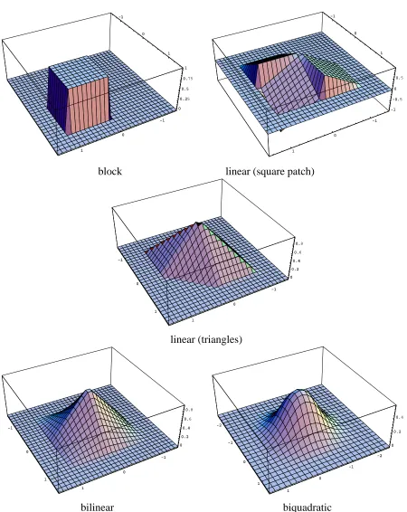
ˆ j). We have studied five different interpolation functions:
1. block:
B
(xy
)=1 on01]2
2. linear:
B
(xy
)= 8 > > > < > > > :(1;
x
;y
) on 01]2
(
x
+1) on ;10]01] and(
y
+1) on 01];10]3. linear on sub-triangles:
B
(xy
)=max(01;max(jx
jjy
jjx
+y
j))4
3.1 Spline-based motion model 7 -1 0 1 -1 0 1 0 0.25 0.5 0.75 1 -1 0 1 -1 0 1 0 0.25 0.5 0. 1 -1 0 1 -1 0 1 -1 -0.5 0 0.5 -1 0 1 -1 0 1 -1 -0.5 0 0.
block linear (square patch)
[image:13.612.78.528.98.664.2]-1 0 1 -1 0 1 0 0.2 0.4 0.6 0.8 -1 0 1 -1 0 1 0 0.2 0.4 0.6 0. linear (triangles) -1 0 1 -1 0 1 0 0.2 0.4 0.6 0.8 -1 0 1 -1 0 1 0 0.2 0.4 0.6 0. -2 -1 0 1 -2 -1 0 1 0 0.2 0.4 -2 -1 0 1 -2 -1 0 1 0 0.2 0. bilinear biquadratic
8 3 General problem formulation
4. bilinear:
B
(xy
)=(1;jx
j)(1;jy
j)on;11]2
5. biquadratic:
B
(xy
)=B
2(x
)B
2(y
)on;12]2, where
B
2(
x
)is the quadratic B-splineFigure 2 shows 3D graphs of the basis functions for the five splines. We also impose the condition that the spline control grid is a regular subsampling of the pixel grid, ˆ
x
j=
mx
i, ˆ
y
j=
my
i, so
that each set of
m
m
pixels corresponds to a single spline patch. This means that the set ofw
ijweights need only be stored for a single patch.
How do spline representations compare to local correlation windows and to regularization? This question has previously been studied in the context of active deformable contours (snakes). The original work on snakes was based on a regularization framework [Kass et al., 1988], giving the snake the ability to model arbitrarily detailed bends or discontinuities where warranted by the data. More recent versions of snakes often employ the B-snake [Menet et al., 1990; Blake et al., 1993] which has fewer control vertices. A spline-based snake has fewer degrees of freedom, and thus may be easier to recover. The smooth interpolation function between vertices plays a similar role to regularization, although the smoothing introduced is not as uniform or stationary.
In our use of splines for modeling displacement fields, we have a similar tradeoff (see Section 9 for more discussion). We often may not need regularization (e.g., in highly textured scenes). Where required, adding a regularization term to the cost function (3) is straightforward, i.e., we can use a first order regularizer [Poggio et al., 1985]
E
1(fu
ˆ klv
ˆklg)=
X
kl (
u
ˆkl ;
u
ˆk ;1l )
2
+(
u
ˆ kl;
u
ˆ kl;1)
2
+ terms in ˆ
v
k l (5)
or a second order regularizer [Terzopoulos, 1986]
E
2(fu
ˆ k :lv
ˆklg) =
h
;2 X
kl (
u
ˆk +1l ;2 ˆ
u
kl +
u
ˆk ;1l )
2
+(
u
ˆ kl+1;2 ˆ
u
kl+
u
ˆ kl;1)
2
+ (6)
(
u
ˆ kl;
u
ˆ kl;1;
u
ˆ k ;1l+
u
ˆ k ;1l;1)
2
+ terms in ˆ
v
k lwhere
h
is the patch size, and we index the spline control vertices with 2D indices(kl
).Spline-based flow descriptors also remove the need for overlapping correlation windows, since each flow estimate(
u
ˆj
v
ˆj) is based on weighted contributions from all of the pixels beneath the
support of its basis function (e.g, (2
m
)(2m
) pixels for a bilinear basis). As we will show in4 Local (general) flow estimation 9
optimal Bayesian estimator for the flow, where the squared pixel errors correspond to Gaussian noise, while the spline model (and any associated regularizers) form the prior model5 [Szeliski,
1989].
Before moving on to our different motion models and solution techniques, we should point out that the squared pixel error function (3) can be generalized to account for photometric variation (global brightness and contrast changes). Following [Lucas, 1984; Gennert, 1988], we can write
E
0 (fu
i
v
ig)=
X
i
I
1(x
i
+
u
i
y
i+
v
i
);
cI
0(x
iy
i)+
b
]2
(7)where
b
andc
are the (per-frame) brightness and contrast correction terms. Both of these parameters can be estimated concurrently with the flow field at little additional cost. Their inclusion is most useful in situations where the photometry can change between successive views (e.g., when the images are not acquired concurrently). We should also mention that the matching need not occur directly on the raw intensity images. Both linear (e.g., low-pass or band-pass filtering [Burt and Adelson, 1983]) and non-linear pre-processing can be performed.4
Local (general) flow estimation
To recover the local spline-based flow parameters, we need to minimize the cost function (3) with respect to thef
u
ˆj
v
ˆjg. We do this using a variant of the Levenberg-Marquardt iterative non-linear
minimization technique [Press et al., 1992]. First, we compute the gradient of
E
in (3) with respect to each of the parameters ˆu
j and ˆv
j,g
u j
@E
@
u
ˆj=2
X
i
e
iG
x iw
ijg
v j@E
@
v
ˆj=2
X
i
e
iG
yi
w
ij
(8)where
e
i=
I
1(x
i+
u
i
y
i+
v
i
);
I
0(x
iy
i) (9)
is the intensity error at pixel
i
,(
G
x
i
G
y
i
)=r
I
1(x
i+
u
i
y
i+
v
i
) (10)
5Correlation-based techniques with overlapping windows do not have a similar direct connection to Bayesian
10 4 Local (general) flow estimation
is the intensity gradient of
I
1at the displaced position for pixeli
, and thew
ij are the sampled valuesof the spline basis function (4). Algorithmically, we compute the above gradients by first forming the displacement vector for each pixel(
u
i
v
i)using (4), then computing the resampled intensity
and gradient values of
I
1at(x
0i
y
0
i
)=(
x
i
+
u
i
y
i+
v
i
), computing
e
i, and finally incrementing the
g
u jand
g
v jvalues of all control vertices affecting that pixel.
For the Levenberg-Marquardt algorithm, we also require the approximate Hessian matrix
A
where the second-derivative terms are left out.6 The matrixA
contains entries of the forma
uu jk = 2 X i@e
i@
u
ˆj@e
i@
u
ˆk=2
X
i
w
ijw
ik(
G
x i ) 2a
uv jk =a
v u jk = 2 X i@e
i@
u
ˆj@e
i@
v
ˆk=2
X
i
w
ijw
ikG
xi
G
y
i (11)
a
v v jk= 2
X
i
@e
i@
v
ˆj@e
i@
v
ˆk=2
X
i
w
ijw
ik(
G
y
i )
2
:
The entries of
A
can be computed at the same time as the energy gradients.What is the structure of the approximate Hessian matrix? The 22 sub-matrix
A
jj
corre-sponding to the terms
a
uu jj,a
uv
jj, and
a
v vjj encodes the local shape of the sum-of-squared difference
correlation surface [Lucas, 1984; Anandan, 1989]. This matrix is often used to compute an updated flow vector by setting
∆
u
ˆ j ∆v
ˆj] T
=;
A
;1 jj
g
u jg
v j ] T (12) [Lucas, 1984; Anandan, 1989; Bergen et al., 1992]. The overallA
matrix is a sparse multi-banded block-diagonal matrix, i.e., sub-blocksA
jkwill be non-zero only if verticesj
andk
both influencesome common patch of pixels.
The Levenberg-Marquardt algorithm proceeds by computing an increment ∆
u
to the current displacement estimateu
which satisfies(
A
+diag(A
))∆u
=;g
(13)where
u
is the vector of concatenated displacement estimatesfu
ˆ jv
ˆjg,
g
is the vector ofconcate-nated energy gradients f
g
uj
g
v
j
g, and
is a stabilization factor which varies over time [Press et al., 1992]. For systems with small numbers of parameters, e.g., if only a single spline patch is6As mentioned in [Press et al., 1992], inclusion of these terms can be destabilizing if the model fits badly or is
4 Local (general) flow estimation 11
being used (Section 5), this system of equations can be solved at reasonable computational cost. However, for general flow computation, there may be thousands of spline control variables (e.g., for a 640480 image with
m
=8, we have 81612104parameters). In this case, iterative
sparse matrix techniques have to be used to solve the above system of equations.7
In our current implementation, we use preconditioned gradient descent to update our flow estimates
∆
u
=;B
;1g
=;
g
ˆ (14)where
B
=A
ˆ +I
, and ˆA
= block diag(A
)is the set of 2 2 block diagonal matrices usedin (12).8 In this simplest version, the update rule is very close to that used by [Lucas, 1984] and
others, with the following differences:
1. the equations for computing the
g
andA
are different (based on spline interpolation) 2. an additional diagonal termis added for stability93. there is a step size
.The step size
is necessary because we are ignoring the off-block-diagonal terms inA
, which can be quite significant. An optimal value forcan be computed at each iteration by minimizing∆
E
(d
)2
d
TAd
;2
d
T
g
i.e., by setting
= (d
g
)=
(d
T
Ad
). The denominator can be computed without explicitly
computing
A
by noting thatd
TAd
=X
i
(
G
x
i
u
i
+
G
y
i
v
i )
2 where
u
i =
X
j
w
iju
ˆjv
i =X
j
w
ijv
ˆjand the(
u
ˆ jv
ˆj)are the components of
d
.To handle larger displacements, we run our algorithm in a coarse-to-fine (hierarchical) fashion. A Gaussian image pyramid is first computed using an iterated 3-pt filter [Burt and Adelson,
7Excessive fill in prevents the application of direct sparse matrix solvers [Terzopoulos, 1986; Szeliski, 1989]. 8The vector ˆ
g
=
B
;1
g
is called the preconditioned residual vector. For preconditioned conjugate gradient descent, the direction vector
d
is set to ˆg
.9A Bayesian justification can be found in [Simoncelli et al., 1991], and additional possible local weightings in
12 5 Global (planar) flow estimation
1983]. We then run the algorithm on one of the smaller pyramid levels, and use the resulting flow estimates to initialize the next finer level (using bilinear interpolation and doubling the displacement magnitudes). Figure 3 shows a block diagram of the processing stages involved in our spline-based image registration algorithm.
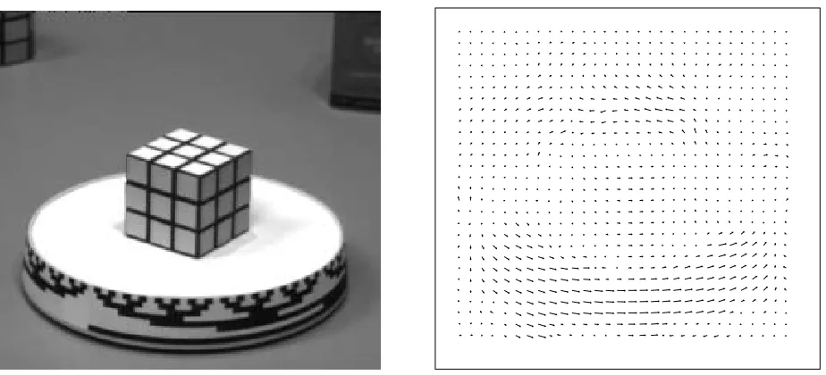
Figure 4 shows an example of the flow estimates produced by our technique. The input image is 256240 pixels, and the flow is displayed on a 3028 grid. We used 1616 pixel spline patches,
and 3 levels in the pyramid, with 9 iterations at each level. The flow estimates are very good in the textured areas corresponding to the Rubik cube, the stationary boxes, and the turntable edges. Flow vectors in the uniform intensity areas (e.g., table and turntable tops) are fairly arbitrary. This example uses no regularization beyond that imposed by the spline patches, nor does it threshold flow vectors according to certainty. For a more detailed analysis, see Section 8.
5
Global (planar) flow estimation
In many applications, e.g., in the registration of pieces of a flat scene, when the distance between the camera and the scene is large [Bergen et al., 1992], or when performing a coarse registration of slices in a volumetric data set [Carlbom et al., 1991], a single global description of the motion model may suffice. A simple example of such a global motion is an affine flow [Koenderink and van Doorn, 1991; Rehg and Witkin, 1991; Bergen et al., 1992]
u
(xy
) = (m
0x
+m
1y
+m
2);x
v
(xy
) = (m
3x
+m
4y
+m
5);y:
(15)The parameters
m
=(m
0:::m
5) Tare called the global motion parameters. Models with fewer degrees of freedom such as pure translation, translation and rotation, or translation plus rotation and scale (similarity transform) are also possible, but they will not be studied in this paper.
To compute the global motion estimate, we take a two step approach. First, we define the spline control vertices ˆ
u
j=(
u
ˆ jv
ˆj) T
in terms of the global motion parameters
ˆ
u
j =2
4
ˆ
x
jy
ˆj 1 0 0 00 0 0
x
ˆjy
ˆj 1 35
m
; 2
4
ˆ
x
jˆ
y
j 35
T
j
m
;
x
ˆj
:
(16)5 Global (planar) flow estimation 13
First Image
Second
Image Controlvertices
Warping (resampling) Spline Interpolation Difference Spatial gradient Flow
gradient HessianFlow
Flow step
(4)
(9) (10)
(8) (12) (13)
?
I
0(x
iy
i)
?
I
1(x
iy
i)
?
I
1(x
i+
u
i
y
i+
v
i ) s ? ?e
i ? (G
x iG
y i ) s ?g
=f(g
u jg
v j )g 6A
=fa
uvjk g
6
?
u
=f(u
ˆ jv
ˆj)g
s
(
u
iv
i [image:19.612.69.514.127.592.2]) 6 ∆
u
i + ?Figure 3: Block diagram of spline-based image registration
14 5 Global (planar) flow estimation
Figure 4: Example of general flow computation
(or simpler) flow, this gives the correct flow at each pixel if linear or bilinear interpolants are used.10
For affine (or simpler) flow, it is therefore possible to use only a single spline patch.11
Why use this two-step procedure then? First, this approach will work better when we generalize our motion model to 2D projective transformations (see below). Second, there are computational savings in only storing the
w
ij for smaller patches. Lastly, we can obtain a better estimate of theHessian at
m
at lower computational cost, as we discuss below.To apply Levenberg-Marquardt as before, we need to compute both the gradient of the cost function with respect to
m
and the Hessian. Computing the gradient is straightforwardg
m@E
@
m
=X
j
@
u
ˆj@
m
@
@E
u
ˆj =X
j
T
T jg
j (17)
where
g
j=(
g
u
j
g
v
j )
T
. The Hessian matrix can be computed in a similar fashion
A
m =@
2E
@
m
T@
m
X
jk
T
Tj
A
jk
T
k (18)where the
A
jk are the 22 submatrices of
A
.10
The definitions of ˆ
u
j and ˆv
jwould have to be adjusted if biquadratic splines are being used.11Multiple affine patches can also be used to track features [Rehg and Witkin, 1991]. Our general flow estimator
5 Global (planar) flow estimation 15
We can approximate the Hessian matrix even further by neglecting the off-diagonal
A
jkmatri-ces. This is equivalent to modeling the flow estimate at each control vertex as being independent of other vertex estimates. When the spline patches are sufficiently large and contain sufficient texture, this turns out to be a reasonable approximation.
To compute the optimal step size
, we letd
=Td
m (19)where
T
is the concatenation of all theT
j matrices, and then set=(
d
g
)=
(d
T
Ad
[image:21.612.220.392.426.481.2])as before.
Figure 5 shows a block diagram of the processing stages involved in the global motion estimation algorithms presented in this and the next section.
Examples of our global affine flow estimator applied to two different motion sequences can be seen in Figures 6 and 7. These two sequences were generated synthetically from a real base image, with Figure 6 being pure translational motion, and Figure 7 being divergent motion [Barron
et al., 1994]. As expected, the motion is recovered extremely well in this case (see Section 8 for
quantitative results).
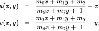
A more interesting case, in general, is that of a planar surface in motion viewed through a pinhole camera. This motion can be described as a 2D projective transformation of the plane
u
(xy
) =m
0x
+m
1y
+m
2m
6x
+m
7y
+ 1;
x
v
(xy
) =m
3x
+m
4y
+m
5m
6x
+m
7y
+ 1;
y:
(20)Our projective formulation12 requires 8 parameters per frame, which is the same number as the
quadratic flow field used in [Bergen et al., 1992]. However, our formulation allows for arbitrarily large displacements, whereas [Bergen et al., 1992] is based on instantaneous (infinitesimal) motion. Our formulation also does not require the camera to be calibrated, and allows the internal camera parameters (e.g., zoom) to vary over time. The price we pay is that the motion field is no longer a linear function of the global motion parameters.
To compute the gradient and the Hessian, we proceed as before. We use the equations
ˆ
u
j =m
0x
ˆj+
m
1y
ˆ j+
m
2m
6x
ˆj+
m
7y
ˆ j+ 1
;
x
ˆ j12In its full generality, we should have an
m
8instead of a 1 in the denominator. The situation
m
8 =0 occurs onlyfor 90
16 5 Global (planar) flow estimation
Control vertices
Global motion
parameters estimatesDepth
Image warping, differencing, and gradient computation (Figure 3) Motion model Motion step Depth step Motion gradient Depth gradient (16,23) (17–18) (25–26)
u
=f(u
ˆ jv
ˆj)g s ? 6 ? ?
I
1I
0A
=fa
uvjk g
s
6 6
g
=f(g
u jg
v j )g s 6 6 ?m
s 6 ∆m
i + ? 6g
m 6A
m ? [image:22.612.72.513.122.593.2]z
=fz
ˆ j g s 6 ∆z
i + ? 6g
z 6A
zFigure 5: Block diagram of global motion estimation
5 Global (planar) flow estimation 17
[image:23.612.74.532.389.620.2]Figure 6: Example of affine flow computation: translation
18 6 Mixed global and local (rigid) flow estimation
ˆ
v
j =m
3x
ˆj+
m
4y
ˆ j+
m
5m
6x
ˆj+
m
7y
ˆ j+ 1
;
y
ˆj (21)
to compute the spline control vertices, and use the B-spline interpolants to compute the flow at each pixel. This flow is not exactly equivalent to the true projective flow defined in (20), since the latter involves a division at each pixel. However, the error will be small if the patches are small and/or the perspective distortion (
m
6m
7) is small.To compute the gradient, we note that
u
ˆj = 1D
j 2 4 ˆx
jy
ˆj 1 0 0 0 ;x
ˆj
N
uj
=D
j ;
y
ˆj
N
u
j
=D
j
0 0 0
x
ˆjy
ˆj 1 ;x
ˆj
N
vj
=D
j ;
y
ˆj
N
vj
=D
j 3
5
m
T
j
m
(22)where
N
u j=
m
0x
ˆ j+
m
1y
ˆ j+
m
2 andN
v
j
=
m
3x
ˆ j+
m
4y
ˆ j+
m
5 are the current numerators of(21),
D
j=
m
6x
ˆ j+
m
7y
ˆ j+1 is the current denominator, and
m
= (m
0:::m
7) T. With this modification to the affine case, we can proceed as before, applying (17)–(19) to compute the global gradient, Hessian, and the stepsize. Thus, we see that even though the problem is no longer linear, the modifications involve simply using an extra division per spline control vertex. Figure 8 shows an image which has been perspectively distorted and the accompanying recovered flow field. The motion is that of a plane rotating around its
y
axis and moving slightly forward, viewed with a wide angle lens.6
Mixed global and local (rigid) flow estimation
A special case of optic flow computation which occurs often in practice is that of rigid motion, i.e., when the camera moves through a static scene, or a single object moves rigidly in front of a camera. Commonly used techniques (direct methods) based on estimating the instantaneous camera egomotion(
R
(!
)t
)and a camera-centered depthZ
(xy
)are given in [Horn and WeldonJr., 1988; Hanna, 1991; Bergen et al., 1992]. This has the disadvantage of only being valid for small motions, of requiring a calibrated camera, and of sensitivity problems with the depth estimates.13
Our approach is based on a projective formulation of structure from motion [Hartley et al., 1992; Faugeras, 1992; Mohr et al., 1993; Szeliski and Kang, 1994]
u
(xy
) =m
0x
+m
1y
+m
8z
(xy
)+m
2m
6x
+m
7y
+m
10z
(xy
)+1;
x
13
6 Mixed global and local (rigid) flow estimation 19
Figure 8: Example of 2D projective motion estimation
v
(xy
) =m
3x
+m
4y
+m
9z
(xy
)+m
5m
6x
+m
7y
+m
10z
(xy
)+1;
y:
(23)This formulation is valid for any pinhole camera model, even with time varying internal camera parameters. The local shape estimates
z
(xy
) are projective depth estimates, i.e., the(xyz
1)coordinates are related to the true Euclidean coordinates(
XYZ
1)through some 3-D projectivetransformation (collineation) which can, given enough views, be recovered from the projective motion estimates [Szeliski, 1994b].14
Compared to the usual rigid motion formulation, we have to estimate more global parameters (11 instead of 6) for the global motion, so we might be concerned with an increased uncertainty in these parameters. However, we do not require our camera to be calibrated or to have fixed internal parameters. We can also deal with arbitrarily large displacements and non-smooth motion. Furthermore, situations in which either the global motion or local shape estimates are poorly recovered (e.g., planar scenes, pure rotation) do not cause any problems for our technique.
A special case of the rigid motion problem is when we are given a pair of calibrated images
14
There is an ambiguity in the shape recovered, i.e., we can add any plane equation to the
z
coordinates,z
0 =ax
+by
+cz
+d
, and still have a valid solution after adjusting them
l. This ambiguity is not a problem for gradient
20 6 Mixed global and local (rigid) flow estimation
(stereo) or a set of weakly calibrated images (only the epipoles in the images are known [Hartley
et al., 1992; Faugeras, 1992]). In either case, we can compute the
m
l, resulting in a simpleestimation problem in
z
(xy
). We can then either proceed to resample (rectify) the images so thatcorresponding pixels lie along scanlines [Hartley and Gupta, 1993], or we can directly work with the original images, proceeding as below but omitting the
m
update step.To compute the global and local flow estimates, we combine several of the approaches developed previously in the paper. First, we compute the 2D flows at the control vertices by evaluating (23) at the vertex locationsf(
x
ˆj
y
ˆj)g. We compute the gradients and Hessian with respect to the global
motion parameters as before, with
T
j = 1D
j 2 4 ˆx
jy
ˆj 1 0 0 0 ;x
ˆj
N
uj
=D
j ;
y
ˆj
N
u
j
=D
j
z
ˆj 0;
z
ˆ jN
u
j
=D
j
0 0 0
x
ˆjy
ˆj 1 ;x
ˆj
N
vj
=D
j ;
y
ˆj
N
v
j
=D
j 0
z
ˆj;
z
ˆj
N
v
j
=D
j 3
5
(24)N
u j=
m
0x
ˆ j+
m
1y
ˆ j+
m
8z
ˆ j+
m
2,N
v
j
=
m
3x
ˆ j+
m
4y
ˆ j+
m
9z
ˆ j+
m
5, andD
j=
m
6x
ˆ j+
m
7y
ˆ j+
m
10z
ˆj+1. The derivatives with respect to the depth estimates ˆ
z
jareg
z j
@E
@
z
ˆj=
@E
@
u
ˆj@
u
ˆj@
z
ˆj +@E
@
v
ˆj@
u
ˆj@
z
ˆj=
g
u
j
m
8;m
10N
u j=D
jD
j +g
v jm
9;m
10N
vj
=D
j
D
j(25) The Hessian matrix
A
z for thez
=fz
ˆj
gparameters has components
a
z jk=(
p
uv =z j ) T
A
jkp
uv =z kwith
p
uv =zj
=(
p
u=z j
p
v =z j ) T (@
u
ˆj@
z
ˆj@
v
ˆj@
z
ˆj )T
:
(26) There are two ways at this point to estimate the
m
andz
parameters. We can take simultaneous steps in ∆m
and ∆z
, or we can alternate steps in ∆m
and ∆z
. The former approach is the one we adopted in [Szeliski, 1994b], since the full Hessian matrix had already been computed thus enabling a regular Levenberg-Marquardt step, and this proved to have faster convergence. In this work, we adopt the latter approach, since it proved to be simpler to implement. We plan to compare both approaches in future work.The performance of our rigid motion estimation algorithm on a sample image sequence is shown in Figure 9. As can be seen, the overall direction of motion (the epipolar geometry) has been recovered well, and the motion estimates look reasonable.15 The computed depth map is
shown in grayscale. The lower right flow field shows the local (general flow) model applied to the same image pair.
15
6 Mixed global and local (rigid) flow estimation 21
(a) (b)
[image:27.612.75.539.127.607.2](c) (d)
Figure 9: Example of 3D projective (rigid) motion estimation
22 7 Multiframe flow estimation
7
Multiframe flow estimation
Many current optical flow techniques use more than two images to arrive at local estimates of flow. This is particularly true of spatio-temporal filtering approaches [Adelson and Bergen, 1985; Heeger, 1987; Fleet and Jepson, 1990]. For example, the implementation of [Fleet and Jepson, 1990] described in [Barron et al., 1994] uses 21 images per estimate. Stereo matching techniques have also successfully used multiple images [Bolles et al., 1987; Matthies et al., 1989; Okutomi and Kanade, 1993]. Using large numbers of images not only improves the accuracy of the estimates through noise averaging, but it can also disambiguate between possible matches [Okutomi and Kanade, 1993].
The extension of our local, global, and mixed motion models to multiple frames is straightfor-ward. For local flow, we assume that displacements between successive images and a base image are known scalar multiples of each other,
u
t(
xy
)=s
t
u
1(
xy
) andv
t
(
xy
)=s
t
v
1(
xy
) (27)i.e., that we have linear flow (no acceleration).16 We then minimize the overall cost function
E
(fu
iv
ig)= X t X i
I
t (x
i +s
t
u
iy
i+
s
t
v
i);
I
0(x
iy
i)]
2
:
(28)
This approach is similar to the sum of sum of squared-distance (SSSD) algorithm of [Okutomi and Kanade, 1993], except that we represent the motion with a subsampled set of spline coefficients, eliminating the need for overlapping correlation windows.
The modifications to the flow estimation algorithm are minor and obvious. For example, the gradient with respect to the local flow estimate ˆ
u
j in (8) becomesg
u j =2 X ts
t X ie
tiG
xti
w
ijwith
e
ti andG
xti being the same as
e
i and
G
x
i with
I
1 replaced byI
t. Given a block of images,
estimating two sets of flows, one registered with the first image and another registered with the last, would allow us to do bidirectional prediction for motion-compensated video coding [Le Gall, 1991]. Examples of the improvements in accuracy due to multiframe estimation are given in Section 8.
16In the most common case, a uniform temporal sampling (
s
t
=
t
) is assumed, but this is not strictly necessary8 Experimental results 23
For global motion estimation, we can either assume that the motion estimates
m
t are relatedby a known transform (e.g., uniform camera velocity), or we can assume an independent motion estimate for each frame. The latter situation seems more useful, especially in multiframe image mosaicing applications. The motion estimation problem in this case decomposes into a set of independent global motion estimation sub-problems.
The multiframe global/local motion estimation problem is more interesting. Here, we can assume that the global motion parameters for each frame
m
t are independent, but that the localshape parameters ˆ
z
j do not vary over time. This is the situation when we analyze multiple arbitraryviews of a rigid 3-D scene, e.g., in the multiframe uncalibrated stereo problem. The modifications to the estimation algorithm are also straightforward. The gradients and Hessian with respect to the global motion parameters
m
tare the same as before, except that the denominatorD
tj is nowdifferent for each frame (since it is a function of
m
t).The derivatives with respect to the depth estimates ˆ
z
jare computed by summing over all framesg
z j= X
t
p
u=ztj
g
u
tj
+
p
v =z
tj
g
vtj (29)
where the
p
u=z tjand
p
v =z tj(which depend on
m
t) and theg
utj
and
g
v tj(which depend on
I
t) are differentfor each frame. Note that we can no longer get away with a single temporally invariant flow field gradient(
g
u
j
g
u
j
)(another way to see this is that the epipolar lines in each image can be arbitrary).
8
Experimental results
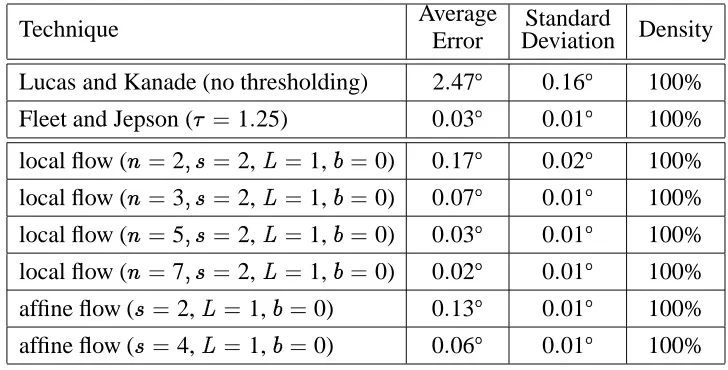
In this section, we demonstrate the performance of our algorithms on the standard motion sequences analyzed in [Barron et al., 1994]. Some of the images in these sequences have already been shown in Figures 4–9. The remaining images are shown in Figures 10–14. We follow the organization of [Barron et al., 1994], presenting quantitative results on synthetically generated sequences first, followed by qualitative results on real motion sequences.
Tables 1–5 give the quantitative results of our algorithms. In these tables, the top two rows are copied from [Barron et al., 1994]. The errors are reported as in [Barron et al., 1994], i.e., by converting flow measurements into unit vector inR
3 and taking the angle between them. The
24 8 Experimental results
Technique AverageError DeviationStandard Density Lucas and Kanade (no thresholding) 2
:
470
:
16100% Fleet and Jepson (
=1:
25) 0:
03
0
:
01100% local flow (
n
=2s
=2,L
=1,b
=0) 0:
17
0
:
02100% local flow (
n
=3s
=2,L
=1,b
=0) 0:
07
0
:
01100% local flow (
n
=5s
=2,L
=1,b
=0) 0:
03
0
:
01100% local flow (
n
=7s
=2,L
=1,b
=0) 0:
02
0
:
01100% affine flow (
s
=2,L
=1,b
=0) 0:
13
0
:
01100% affine flow (
s
=4,L
=1,b
=0) 0:
06
0
:
01 [image:30.612.123.487.107.292.2]100% Table 1: Summary of Sinusoid 1 results
Sinusoid 1 image (single level, 9 iterations) to 30 seconds for the 300300 Nasa Sequence (three
levels, rigid flow, 9 iterations per level).
From the nine algorithms in [Barron et al., 1994], we have chosen to show the Lucas and Kanade results, since their algorithm most closely matches ours and generally gives good results, and the Fleet and Jepson algorithm since it generally gave the best results. The most salient difference between our (local) algorithm and Lucas and Kanade is that we use a spline representation, which removes the need for overlapping correlation windows, and is therefore much more computationally efficient. The biggest difference with Fleet and Jepson is that they use the whole image sequence (20 frames) whereas we normally use only two (multiframe results are shown in Table 3).
As with many motion estimation algorithms, our algorithms require the selection of some relevant parameters. The most important of these are:
n
[2] the number of framess
[1] the step between frames, i.e., 1 = consecutive frames, 2 = every other frame,:::
m
[16] the size of the patch (width and height,m
2pixels per patch)L
[3] the number of coarse-to-fine levelsb
[3] the amount of initial blurring (# of iterations of a box filter)Unless mentioned otherwise, we used the default values shown in brackets above for the results in Tables 1–5. Bilinear interpolation was used for the flow fields.
8 Experimental results 25
Figure 10: Sinusoid 1 and Square 2 sample images
2 (Figure 10). The translations in these sequences are(1
:
5850:
863)and(1:
3331:
333)pixels perframe, respectively. Our local flow estimates for the sinusoid sequence are very good using only two frames (Table 1), and beat all other algorithms when 7 or more frames are used. For this sequence, we use a single level and no blurring and take a (
s
= 2)frame step for better results.To help overcome local minima for the multiframe (
n >
2) sequences, we solve a series of easier subproblems [Xu et al., 1987]. We first estimate two-frame motion, then use the resulting estimate to initialize a three-frame estimator, etc. Without this modification, performance on longer (e.g.,n
=8) sequences would start to degrade because of local minima. The global affine model motionestimator performs well.
For the translating square (Table 2), our results are not as good because of the aperture problem, but with additional regularization, we still outperform all of the nine algorithms studied in [Barron
et al., 1994]. To produce the sparse flow estimates (9–23% density), we set a threshold
T
e onthe minimum eigenvalues of the local Hessian matrices
A
jj interpolated over the whole grid (thisselects areas where both components of the motion estimate are well determined). The affine (global) flow for the square sequence works extremely well, outperforming all other techniques by a large margin.
26 8 Experimental results
Technique AverageError DeviationStandard Density Lucas and Kanade (
25:
0) 0:
14
0
:
107.9% Fleet and Jepson (
=2:
5) 0:
18
0
:
1312.6% local flow (
T
e=10
4) 2
:
981
:
169.1% local flow (
s
=2T
e
=10
4) 1
:
781
:
0710.1% local flow (
s
=21 =103
T
e
=10
4) 0
:
470
:
2723.8% local flow (
s
=21 =104) 0
:
130
:
10100%
affine flow 0
:
030
:
02100% Table 2: Summary of Square 2 results
Technique AverageError DeviationStandard Density Lucas and Kanade (
2 5:
0) 0:
56
0
:
5813.1% Fleet and Jepson (
=1:
25) 0:
23
0
:
1949.7% local flow (
n
=2) 0:
35
0
:
34100% local flow (
n
=3) 0:
30
0
:
30100% local flow (
n
=5) 0:
24
0
:
15100% local flow (
n
=8) 0:
19
0
:
10100%
affine flow 0
:
170
:
12 [image:32.612.149.464.451.614.2]8 Experimental results 27
Technique AverageError DeviationStandard Density Lucas and Kanade (
2 5:
0) 1:
65
1
:
4824.3% Fleet and Jepson (
=1:
25) 0:
80
0
:
7346.5% local flow (
s
=4L
=1) 0:
98
0
:
74100% local flow (
s
=4L
=11 =103) 0
:
780
:
47100%
affine flow 2
:
510
:
77 [image:33.612.132.478.108.235.2]100% Table 4: Summary of Diverging Tree results
Technique AverageError DeviationStandard Density Lucas and Kanade (
2 5:
0) 3:
22
8
:
928.7% Fleet and Jepson (
=1:
25) 5:
28
14
:
3430.6% local flow (
s
=2,T
e
=3000) 2
:
195
:
8623.1% local flow (
s
=2,T
e
=2000) 3
:
067
:
5439.6% local flow, cropped (
s
=2) 2:
45
3
:
05100% rigid flow, cropped (
s
=2) 3:
77
3
:
32100% Table 5: Summary of Yosemite results
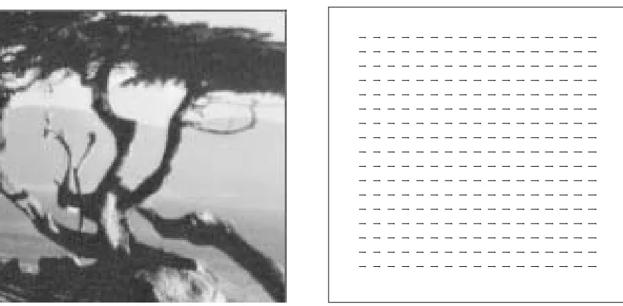
7) and synthetic (global) motion. Our results on the translating motion sequence (Table 3) are as good as any other technique for the local algorithm (note the difference in density between our results and the previous ones), and outperform all techniques for the affine motion model, even though we are just using two frames from the sequence. The results on the diverging tree sequence are good for the local flow, but not as good for the affine flow. These results are comparable or better than the other techniques in [Barron et al., 1994] which produce 100% density.
The final motion sequence for which quantitative results are available is Yosemite (Figure 11 and Table 5). The images in this sequence were generated by Lynn Quam using his texture mapping algorithm applied to an aerial photograph registered with a digital terrain model. There is significant occlusion and temporal aliasing, and the fractal clouds move independently from the terrain. Our results on this more realistic sequence are better than any of the techniques in [Barron
et al., 1994], even though we again only use two images. As expected, the quality of the results
[image:33.612.151.463.268.414.2]28 8 Experimental results
Figure 11: Yosemite sample image and flow (unthresholded)
the density of the estimates and their quality. We also ran our algorithm on just the lower 176 (out of 252) rows of the images sequence. The dense (unthresholded) estimates are comparable to the thresholded full-frame estimates. Unfortunately, the results using the rigid motion model were slightly worse.
To conclude our experimental section, we show results on some real motion sequences for which no ground truth data is available. The SRI Trees results have already been presented in Figure 9 for both rigid and local (general) flow. Figure 12 shows the NASA Sequence in which the camera moves forward in a rigid scene (there is significant aliasing). The motion estimates look quite reasonable, as does the associated depth map (not shown).17 Figure 13 shows the sparse
flow computed for the Rubik Cube sequence (the dense flows were shown in Figure 4). The areas with texture and/or corners produce the most reliable flow estimates. Finally, the results on the Hamburg Taxi are shown in Figure 14, where the independent motion of the three moving cars can be clearly distinguished. Overall, these results are comparable or better than those shown in [Barron et al., 1994].
Much work remains to be done in the experimental evaluation of our algorithms. In addition to systematically studying the effects of the parameters
n
,s
,m
,L
, andb
(introduced previously), we plan to study the effects of different spline interpolation functions, the effects of different preconditioners, and the usefulness of using conjugate gradient descent.17
8 Experimental results 29
[image:35.612.72.541.121.365.2]/s.23.pp > /dev/null] --- rigid flow [compute_flow -d64 -n9 -l3 -p -s8 -w3 -y -e8 -Dtmp2.dump -M8 -L0,10,0 -Z1.0 nasa/s.19.pp nasa/s.23.pp > / Image size 300 x 300 Subsampled by 8 scaled by 3.000
[image:35.612.74.542.425.636.2]Figure 12: NASA Sequence, rigid flow
30 9 Discussion
Figure 14: Hamburg Taxi sequence, dense local flow
9
Discussion
The spline-based motion estimation algorithms introduced in this paper are a hybrid of local optic flow algorithms and global motion estimators, utilizing the best features of both approaches. Like other local methods, we can produce detailed local flow estimates which perform well in the presence of independently moving objects and large depth variations. Unlike correlation-based methods, however, we do not assume a local translational model in each correlation window. Instead, the pixel motion within each of our patches can model affine or even more complex motions (e.g., bilinear interpolation of the four spline control vertices can provide an approximation to local projective flow). This is especially important when we analyze extended motion sequences, where local intensity patterns can deform significantly. Our technique can be viewed as a generalization of affine patch trackers [Rehg and Witkin, 1991; Shi and Tomasi, 1994] where the patch corners are stitched together over the whole image.
Another major difference between our spline-based approach and correlation-based approaches is in computational efficiency. Each pixel in our approach only contributes its error to the 4 spline control vertices influencing its displacement, whereas in correlation-based approaches, each pixel contributes to
m
2overlapping windows. Furthermore, operations such as inverting the local Hessian or computing the contribution to a global model only occur at the spline control vertices, thereby providing anO
(m
2
)speedup over correlation-based techniques. For typically-sized patches
9 Discussion 31
resolution of the computed flow field, especially when compared to locally adaptive widows [Okutomi and Kanade, 1992] (which are extremely computationally demanding). However, since window-based approaches produce highly correlated estimates anyway, we do not expect this difference to be significant.
Compared to spatio-temporal filtering approaches, we see a similar improvement in compu-tational efficiency. Separable filters can reduce the complexity of computing the required local features from
O
(m
3
)to
O
(m
), but these operations must still be performed at each pixel.Further-more, a large number of differently tuned filters are normally used. Since the final estimates are highly correlated anyway, it just makes more computational sense to perform the calculations on a sparser grid, as we do.
Because our spline-based motion representation already has a smoothness constraint built in, regularization, which requires many iterations to propagate local constraints, is not usually necessary. If we desire longer-range smoothness constraints, regularization can easily be added to our framework. Having fewer free variables in our estimation framework leads to faster convergence when iteration is necessary to propagate such constraints.
Turning to global motion estimation, our motion model for planar surface flow can handle arbitrarily large motions and displacements, unlike the instantaneous model of [Bergen et al., 1992]. We see this as an advantage in many situations, e.g., in compositing multiple views of planar surfaces [Szeliski, 1994a]. Furthermore, our approach does not require the camera to be calibrated and can handle temporally-varying internal camera parameters. While our flow field is not linear in the unknown parameters, this is not significant, since the overall problem is non-linear and requires iteration.
Our mixed global/local (rigid body) model shares similar advantages over previously devel-oped direct methods: it does not require camera calibration and can handle time-varying camera parameters and arbitrary camera displacements. Furthermore, experimental evidence from some related structure from motion research [Szeliski, 1994b] suggests that our projective formulation of structure and motion converges more quickly than traditional Euclidean formulations.