DETECTION ENVIRONMENT FORMATION METHOD FOR ANOMALY DETECTION SYSTEMS

(1)

ISSN: 1992-8645 www.jatit.org E-ISSN: 1817-3195

4439

METAHEURISTIC APPROACH USING GREY WOLF

OPTIMIZER FOR FINDING STRONGLY CONNECTED

COMPONENTS IN DIGRAPHS

1_{ALA'A AL-SHAIKH,}2_{BASEL A. MAHAFZAH,}3_{MOHAMMAD ALSHRAIDEH}

Department of Computer Science, King Abdullah II School of Information Technology, The University of Jordan, Amman 11942, Jordan

E-mail: 1_{[email protected],}2_{[email protected],}3_{[email protected]}

ABSTRACT

Finding strongly connected components (SCCs) in a directed graph (digraph) has been investigated extensively. Tarjan’s algorithm is the most fundamental method of finding SCCs in digraphs that uses Depth-First Search (DFS) and it has a linear time complexity. On the other hand, the Forward-Backward (FW-BW) algorithm is another well-known method that is based on the divide-and-conquer approach, yet it is time consuming. In this paper, we introduce a new approach for finding the SCCs in digraphs in linear time using Grey Wolf Optimizer (GWO), which is a recent metaheuristic algorithm. Experimental results show that finding SCCs using GWO outperforms FW-BW in terms of run time. In this context, GWO achieved 62.27% average run time improvement over FW-BW. Furthermore, average solution quality (accuracy) from GWO compared to the exact algorithm FW-BW is 97.57%.

Keywords: Grey Wolf Optimizer; Strongly Connected Components; Metaheuristic Algorithms; Optimization Problem; Forward-Backward Algorithm

1. INTRODUCTION

Finding Strongly Connected Components (SCCs) in directed graphs (digraphs) has many applications, such as networks and communications, social networks, data mining, compilers, and much more [1] [2]. It has intensively been studied and researched due to its vitality and importance especially in analyzing graphs.

Formally, let 𝐺 = (𝑉, 𝐸) be a digraph, such that 𝑉 = {𝑣 , 𝑣 , … , 𝑣 } is a set of vertices (nodes) in 𝐺, and 𝐸 = {𝑒 , 𝑒 , … , 𝑒 } is a set of unweighted edges in 𝐺, such that each edge 𝑒 connects only two vertices of 𝑉 together 𝑣 and 𝑣. The existence of a directed edge between two vertices is expressed as 𝑣 → 𝑣, or (𝑣 , 𝑣 ) ∈ 𝐸, and is said that there exists and edge from vertex 𝑣 to vertex 𝑣, or alternatively, vertex 𝑣 is adjacent to vertex 𝑣.

A path may exist between two vertices 𝑣 and 𝑣 , expressed 𝑣 ⇒ 𝑣∗ , which means that vertex 𝑣 is reachable from vertex 𝑣 by a sequence of

distinct vertices 𝑣 , 𝑣 , 𝑣 , …; that is the path 𝑃 is a sequence of vertices 𝑣 , 𝑣 , 𝑣 , 𝑣 , … , 𝑣 [3]. Based on the path definition, a SCC is defined in Definition 1.

Definition 1. A Strongly Connected Component (SCC) is a disjoint set of vertices such that there exists a path from every vertex to every other vertex in the same SCC [2].

A digraph is strongly connected if there is only one SCC in that digraph. In other words, a digraph is strongly connected if there exists a path from every vertex to every other vertex in the digraph [4].

Definition 2. A Trivial SCC is a SCC that contains only one vertex [5].

Based on Definition 2, the smallest-allowed SCC size is 1. In other words, a vertex by itself is considered a SCC.

(2)

4440 Although there were some previous methods used to find SCCs in digraphs, but none of them was linear. However, despite its linearity, several algorithms followed the Tarjan’s algorithm trying to solve the problem using different techniques that can be easily parallelized, due to the P-Complete nature of depth-first search, which is the basis of the Tarjan’s algorithm, which means that depth-first search is inherently sequential and is hard to parallelize [7].

The common feature between all the algorithms that tried to find the SCCs in digraphs is that they all tried to find parallel solutions. Despite the efficiency of the solutions in terms of parallel run time, their sequential run time was rather higher than that of the Tarjan’s algorithm.

1.1 Problem Statement

In this paper, we introduce a new approach for finding the SCCs in digraphs by expressing the problems as an optimization problem and using optimization techniques to find solution to that problem. Basically, optimization techniques are used to solve NP-Complete problems [8]. Nevertheless, we look at finding the SCCs in a digraph as a maximization problem, as follows:

𝑚𝑎𝑥𝑖𝑚𝑧𝑒 𝑆𝐶𝐶, 𝑠𝑢𝑐ℎ 𝑡ℎ𝑎𝑡 𝑆𝐶𝐶 ⊆ 𝑉

𝑠𝑢𝑏𝑗𝑒𝑐𝑡 𝑡𝑜 ∀𝑢, 𝑣 ∈ 𝑆𝐶𝐶(∃𝑢⇒ 𝑣 ∧ 𝑣∗ ⇒ 𝑢)∗

The objective is to maximize the SCC iteratively. This maximization is controlled by the constraint that each two vertices in the same SCC are mutually reachable by each other.

We use Grey Wolf Optimizer (GWO) [9] for the first time to find the SCCs in a digraph. Then, we compare it with FW-BW [2], a well-known algorithm for finding SCCs in digraphs.

Like all other metaheuristics, GWO is used to solve optimization problems by trying to find local optimal solutions rather than global optimal solutions [10]. By global optimal solutions we refer to exact solutions, while local optimal refers to satisfactory solutions that are not exact. The compromise between local and global optimal solutions is in favor of reducing the time required to find the solution.

In fact, there are several factors that motivate us for using metaheuristic algorithms, such as GWO, to find SCCs in digraphs, such as:

 Metaheuristic algorithms are very fast in returning solutions, albeit solutions are local

optimal, but still they are satisfactory and do not require too much time, and thus the time in which a metaheuristic algorithm returns a solution is much lower than that required by the search techniques such as Depth-Fist Search (DFS) or Breadth-First Search (BFS).

 Metaheuristic algorithms are easy to design, implement, and understand. On the other hand, the exact algorithms used to find SCCs in digraphs, they are very difficult to understand, trace, and implement.

 Metaheuristic algorithms do not require too much resources. Consider DFS which requires a large amount of stack and intensive use of memory locations, in addition to great deal of backtracking and computation.

 Metaheuristic algorithms are easy to parallelize. On the other hand, DFS and BFS are P-Complete and thus there are extremely hard to parallelize.

The remainder of this paper is organized as follows: in Section 2, we provide some literature review related to SCC, metaheuristics, and GWO. In Section 3, we present the methodology used to conduct this research, in which we discuss both FW-BW and GWO algorithms including the algorithm design and asymptotic run time complexities. Section 4 presents the experimental results and their discussion. Finally, conclusions are made in Section 5 in addition to suggesting some future work.

2. RELATED WORK

Robert Tarjan [6] was the first to introduce a linear time solution for finding SCCs using DFS. Despite its linear time, the Tarjan’s method is criticized because of the difficulty to parallelize it, especially that it is based on the P-Complete DFS. Later, a divide-and-conquer algorithm was introduced by Lisa K. Fleischer et al [2]. The run time complexity of the later-referred-to algorithm as Forward-Backward (FW-BW) [11] is logarithmic in digraphs where degrees of vertices are bounded by constant. Nevertheless, FW-BW is a time-consuming algorithm as long finding a single SCC in the graph is O(𝑉 + 𝐸).

(3)

4441 The FW-BW algorithm was then reconsidered by S. Hong et al [11] and introduced a solution to parallelize it by adding some extensions to it. Their results achieved more than 29x parallel speedup over the sequential algorithm.

Most enhancement efforts to the problem of finding SCCs in digraphs were concentrated around finding parallel solutions that speedup the processing. Unlike our metaheuristic approach, we concentrate on finding a speed-efficient sequential algorithm. Afterwards, parallelization to the metaheuristic approach can be introduced, so as we can get a reasonable sequential run time as well as parallel speedup.

David J. Pearce introduced a space-efficient algorithm to find SCCs [13]. The author noticed that the space requirement of the Tarjan’s algorithm is too high especially when dealing with real world application where graph sizes are very large. He introduced a solution to the Tarjan’s algorithm that reduces the memory requirements. SCCs were also used in social network analysis by S. Dhingra et al [1]. They observed that advertising companies on social networks target everybody but that causes them losing some users who feel uncomfortable being targeted in an unobjective manner. They claim a 15% loss of audience in response to 10% increase in the advertising behavior. This is considered a huge amount of loss provided that the number of social networks users exceeds billions [14]. They proposed to apply the detection of SCC in social network graph (SNG) to group users of a certain social network based on some criteria in order to target the intended groups only.

Almost all current methods of finding SCCs in digraphs use one of two approaches: DFS (or BFS), or divide-and-conquer, or a combination of the two. However, these two approaches depend heavily on the capabilities of the machines on which the algorithms will run and the programming language in which the algorithms are written. Because of the recursive nature of the two approaches, they incorporate an extensive use of the machine’s stack memory, which might lead to stack overflow problems. Furthermore, it also limits the type of programming languages that can be used to implement those algorithms. For instance, not all languages support Tail-Call Optimization (TCO), such as Java, C#, PHP, Python, etc. Consequently, programmers are

forced to write their codes in loops to avoid the stack overflow problem.

Metaheuristics are high-level frameworks that are used as guidelines for algorithmic designs [10]. Unlike heuristic algorithms, metaheuristics are problem independent and used to express how to find a heuristic solution to an optimization problem [15]. Examples of well-known heuristic search algorithms are: Local search [16], A* algorithm [17], and IDA* [18].

Metaheuristics are classified into single-solution based and population-based [19]. Single-solution-based metaheuristics are only concerned with one solution and keeps on enhancing that solution by making more and more iterations until the algorithm stops. On the other hand, population-based metaheuristics start with a population that comprises a number of individuals (or initial solutions) and the operators of the algorithm are applied to all, or selected, individuals of the populations which results in better solutions.

Unlike the current approaches, our approach is based on using a metaheuristic approach rather than the DFS (or BFS), or divide-and-conquer approach. All metaheuristic algorithms consist of three phases: (1) initialization, (2) iteration, and (3) finalization [9]. Accordingly, a metaheuristic algorithm uses a simple loop statement that iterates several times before it stops upon meeting a predetermined stopping criterion. Thus, there is no more recursion and dependence on the specifications of both the machine and programming language, and there are no more hardware problems, such as stack overflow, also the expected run time of the algorithm is faster.

Undoubtedly, parallelizing metaheuristic algorithms does not incur a huge overhead compared to DFS-based methods. Also, it does not require a special type of parallel architecture as in the divide-and-conquer approach. Metaheuristic algorithms can run sequentially on one machine or in parallel on shared-memory or distributed memory machines.

(4)

4442 Optimization is used to solve many problems in computer science, artificial intelligence, control systems [20], meteorology [21], Internet and cloud computing [8] [22].

Metaheuristics were also used in software engineering discipline. M. Alshraideh et al. used Genetic Algorithm (GA) to generate test data to execute branches in programs [23]. They outperformed other approaches that use single population in terms of search effectiveness, execution time, and number of executions. Moreover, in the field of databases, M. Alshraideh et al. used GA to test exception codes in Jordan University Hospital database [24]. In another work, M. Alshraideh et al. used GA to test oracle stored program units written in PL/SQL [25].

Grey Wolf Optimizer (GWO) is a population-based metaheuristic inspired by the living style and hunting behaviors of grey wolves (or Canis lupus) and was introduced by Mirjalili et al [26]. GWO is used extensively in research to solve too many optimization problems.

Naturally, a pack of grey wolves can be divided into four types [9]:

1. Alpha (𝛼): wolves that are dominants of the pack. These are the wolves of highest rank in the pack and they are responsible of the decision making.

2. Beta (𝛽): the subordinate wolves that are in the second level of hierarchy and help alpha wolves in decision making.

3. Delta (𝛿): wolves that are subordinate to both alpha and beta wolves, but they are dominant to the omega wolves.

4. Omega (𝜔): the wolves in the lowest level of hierarchy. They obey all dominant wolves in the pack.

Practically, the four types of wolves represent the GWO solutions. Alpha wolves (𝛼) represent the best solution, beta (𝛽) represent the second-best solution, delta (𝛿) is the third best solution, and finally omega (𝜔) are the remaining solutions [26].

GWO was used in research to find solution to different optimization problems and finding solutions to real-world applications. A. Shaheen et al. [9] used GWO to solve the travelling salesman problem (TSP) and it is compared with solutions based on chemical reaction optimization (CRO) and GA. They also introduced a parallelization

approach for their GWO solution in a later work [27] over a hypercube interconnection network.

A hybrid approach between GWO and Whale Optimization (WO) was introduced by A. Hudaib et el [28]. The approach was named as WGW and was used to prioritize software requirements. Accuracy of the proposed approach recorded 91%. MAXFLOW-GWO is a solution to the maximum flow problem using GWO which is introduced by R. Masadeh et al [29]. They tested their work on datasets with 50 to 1000 vertices. They compared their results with results of the Ford-Fulkerson’s approach to solve this problem. Results showed that MAXFLOW-GWO outperformed Ford-Fulkerson’s in terms of run time.

Furthermore, GWO has also found a foothold in networking, especially in wireless sensor networks (WSN) area. Because sensor nodes show continuous power dissipation through their lifetime [30], a huge amount of work has been established around eliminating the power dissipation, in which optimization played an important role. In this context, GWO was used to offer a solution to the node localization problem in WSNs [31] in order to position unknown nodes in correct geographical locations. GWO was also used to design power-efficient protocols for WSNs [32], enhance the area coverage of the sensor nodes [33], cluster formation [34], cluster head selection [35], and many more.

3. METHODOLOGY

(5)

4443 3.1 FW-BW Algorithm

The FW-BW algorithm is based on both Lemma 1 and Lemma 2 [2].

Let 𝐺(𝑉, 𝐸) be a digraph, such that 𝑉 is the set of vertices in 𝐺 and 𝐸 is the set of edges in 𝐺, then Lemma 1 withstands [12].

Lemma 1. With respect to a given vertex 𝑣 in the digraph 𝐺, such that 𝑣 ∈ 𝑉, there exists three sets:

1. 𝑃𝑟𝑒𝑑(𝐺, 𝑣): the set of predecessors of vertex 𝑣

in the digraph 𝐺, such that 𝑃𝑟𝑒𝑑(𝐺, 𝑣) = {𝑢 ∈ 𝑉|𝑢⇒ 𝑣}∗ .

2. 𝐷𝑒𝑠𝑐(𝐺, 𝑣): the set of descendants from vertex

𝑣 in the digraph 𝐺, such that 𝐷𝑒𝑠𝑐(𝐺, 𝑣) =

{𝑤 ∈ 𝑉|𝑣⇒ 𝑤}∗ .

3. 𝑅𝑒𝑚(𝐺, 𝑣): the remainder set that contains all

the vertices that are not predecessors or descendants of 𝑣 in the digraph 𝐺, such that

𝑅𝑒𝑚(𝐺, 𝑣) = {𝑥 ∈ 𝑉|𝑥 ⇏∗ 𝑣⋁𝑣 ⇏∗ 𝑥}∎

Based on these three sets, a SCC can be formed according to Lemma 2 [2].

Lemma 2. A SCC in the digraph 𝐺 that contains the vertex 𝑣, denoted 𝑆𝐶𝐶(𝐺, 𝑣) is formed by the intersection between 𝑃𝑟𝑒𝑑(𝐺, 𝑣) and 𝐷𝑒𝑠𝑐(𝐺, 𝑣). i.e. 𝑆𝐶𝐶(𝐺, 𝑣) = 𝑃𝑟𝑒𝑑(𝐺, 𝑣) ∩ 𝐷𝑒𝑠𝑐(𝐺, 𝑣) ∎

The FW-BW algorithm is presented in Algorithm 1. The algorithm starts in line 2 by setting the stopping criteria which stops splitting the digraph and returns in order for the backtracking to start. In line 3, a vertex is selected randomly from the digraph. In line 4, we create a set of all vertices that can reach vertex 𝑣, i.e. predecessors of 𝑣, which was randomly selected in the previous line. All the vertices that are reachable from vertex 𝑣, i.e. descendants from 𝑣, are assigned to the set BW in line 5.

According to Lemma 2, line 6 of Algorithm 1 performs an intersection between the forward component (FW) and backward component (BW). In lines 8-10, the digraph is split into three distinct parts, the first contains all vertices that are in FW but not in the SCC just found (S), expressed as

𝐹𝑊 ∖ 𝑆. The second contains all vertices in BW

but not in S, i.e. 𝐵𝑊 ∖ 𝑆. Finally, the last part contains all vertices that are in the graph but neither in FW nor in BW, i.e. the remaining vertices, expressed 𝑑𝑖𝑔𝑟𝑎𝑝ℎ ∖ (𝐹𝑊 ∪ 𝐵𝑊). The run time complexity of Algorithm 1 is O(𝑉𝑙𝑜𝑔𝑉) such that 𝑉 is the number of vertices in the digraph

𝐺 in which all digraph degrees are bounded by a constant [2].

Algorithm 1 FW-BW(digraph)

Input: digraph – input digraph

Output: SCC

1: begin

2: if empty(digraph) then return;

3: v = random(digraph);

4: FW = Pred(digraph, v);

5: BW = Desc(digraph, v);

6: S = FW ∩ BW;

7: SCC = SCC ∩ S;

8: FW-BW(FW\S);

9: FW-BW(BW\S);

10: FW-BW(digraph\(FW ∪ BW));

11: end;

3.2 Grey Wolf Optimizer (GWO)

In the following subsections we introduce our algorithmic design for using GWO to find SCCs in digraphs as well as introducing an analytical analysis of the run time complexity of the GWO algorithm.

3.2.1 Algorithm Design

Algorithm 2 lists the steps followed to find the SCCs using GWO. The algorithm starts by generating an initial population in line 2. The size of the population is determined by the parameter

𝑎𝑔𝑒𝑛𝑡𝑠. Each item in the population is called an

agent and has a fitness value. Thus, according to our problem, an agent is a SCC, and therefore the fitness of the agent is the number of vertices contained in that agent.

Initially, each agent is assigned a random vertex. In other words, initial population contains trivial SCCs (or trivial agents). This ensures that all agents contain feasible initial solutions and eliminates the need to perform a feasibility check whenever an agent is generated, which in turn reduces that time required by the algorithm’s initialization phase.

The initial population is then sorted in a non-increasing order based on the fitness values of agents. This is a necessary step so as we can select the best three agents in the population and assign them to 𝛼, 𝛽, and 𝛿 respectively, as shown in lines 3-6.

(6)

4444 descendent from the selected vertex 𝑣 , i.e. that is vertex 𝑣 can be reached, (3) find the set BW that contains all vertices that are predecessors of the selected vertex 𝑣 according to Lemma 1, i.e. that is vertex 𝑣 is reachable from, and (4) based on Lemma 2, create a component S as a results of intersecting

both FW and BW sets, such that 𝑆 = 𝐹𝑊 ∩ 𝐵𝑊. These steps are summarized in the find_solution_by_agent() function and they are investigated in details in Algorithm 3.

Algorithm 2 GWO(digraph, maxIterations, agents)

Input: digraph - directed graph, maxIterations - maximum iterations,

agents – number of agents

Output: Strongly Connected Components (SCCs)

1: begin

2: generate_population(agents);

3: sort_population(DESC);

4: alpha = population[0];

5: beta = population[1];

6: delta = population[2];

7: for i = 1 to maxIterations

8: for j = 1 to agents

9: current_agent = population[j];

10: new_agent = find_solution_by_agent(current_agent); //call Algorithm3

11: population[j] = new_agent ∪ current_agent;

12: end for;

13: sort_population(DESC); 14: alpha = population[0]; 15: beta = population[1]; 16: delta = population[2]; 17: end for;

18: output_best_solution(); 19: end;

In line 11, the solution of the new agent is then joined with the solution of the original agent using a union operator and the result of the union operation is set to replace the original agent that was used to generate this new agent.

Again, in lines 13-16, the population is sorted in a non-increasing order in terms of the fitness values of the agents, and the first three agents are selected as 𝛼, 𝛽, and 𝛿, respectively.

The steps in lines 7-16 of Algorithm 2 are repeated 𝑚𝑎𝑥𝐼𝑡𝑒𝑟𝑎𝑡𝑖𝑜𝑛𝑠 times in order for the whole algorithm to complete and a solution is returned (line 18).

Algorithm 3 lists the steps required by the function find_solution_by_agent(). The algorithm creates two partial solutions FW and BW according to Lemma 1 and Lemma 2 in lines 3 and 4, respectively. It is noteworthy, that we use the digraph 𝐺 in line 3 to create a forward component by finding all vertices that are descendant from the vertex 𝑣. Similarly, we use the transpose graph 𝐺 to find all components that are descendant from the vertex 𝑣 in 𝐺 , i.e. the predecessors of 𝑣.

The function create_component() is used to create a component starting from the vertex 𝑣 passed to the function as a parameter. Initially, an empty component is created in line 14. In line 17, the selected vertex is added to the component. In lines 18-20, we enumerate all vertices that are reachable from the selected vertex, and they are added to the component one by one if they are not already included. In line 21, another random vertex is selected, and further iterations are made until there are no more vertices to be selected. The two partial components are then intersected using an intersection operator in line 5. In line 6, a new SCC is returned.

3.2.2 Run Time Complexity

(7)

4445

Algorithm 3 find_solution_by_agent(agent, G, GT₎

Input: agent – the selected agent, G – input digraph,

GT_{– transpose of the input digraph}

Output: agent – an output agent that represents a SCC

1: begin

2: vstart = select_random_vertex(agent);

3: FW = create_component(G, vstart);

4: BW = create_component(GT_{, v}_start_);

5: newAgent = FW ∩ BW;

6: return newAgent;

7: end;

8:

9: Function create_component(G, vstart)

10: begin

11: // G – input digraph, vstart – starting vertex

12: // component – a partial solution

13: v = vstart;

14: component = null; 15: while (v <> null) 16: begin

17: component.add(v);

18: for each adj_vertex ∈ adj[vertex] and adj_vertex ∉ component

19: component.add(adj_vertex); 20: end for;

21: v = random(adj[vertex]); 22: end while;

23: return component; 24: end function;

Lemma 3. The run time complexity of Algorithm 3 is 𝑂(𝑉 + 𝐸).

Proof. We start by finding the complexity of create_component() function. In the worst-case scenario, there exists a path from every vertex to every other vertex in the digraph. This means that all the vertices of the digraph will be explored, and thus the body of the while loop will execute 𝑉 times. Consequently, the loop at lines 18-20 will make 𝐸 iterations. Eventually, there will be 𝑉 + 𝐸 iterations made between the lines 15-22. We designed the union and intersection operators to use Boolean arrays, which resulted in a linear run time complexity. Since the intersection operator in line 5 of Algorithm 3 is used to intersect two partial components together, and as long each component may have all the vertices of the digraph in the worst case, i.e. if the digraph is strongly connected, then the complexity of the intersection operator in line 5 is O(𝑉). Now, let 𝐸(𝐿 ) be the effort of selecting a random vertex from the agent which is constant and is given by O(1), 𝐸(𝐹𝑊) and 𝐸(𝐵𝑊) the effort of finding the first and second partial solutions respectively which equals O(𝑉 + 𝐸) each, 𝐸(∩) the effort of the intersection operator which equals (𝑉), and 𝐸(𝐿 ) is the effort of the return statement at line 6 of Algorithm 3 which is

constant and equals O(1). Then, the run time complexity (effort) of Algorithm 3, denoted 𝐸(𝐴 ) is computed as follows:

𝐸(𝐴 ) = 𝐸(𝐿 ) + 𝐸(𝐹𝑊) + 𝐸(𝐵𝑊) +

𝐸(∩) + 𝐸(𝐿 )

= O(1) + O(𝑉 + 𝐸) + O(𝑉 + 𝐸) +

O(𝑉) + O(1)

= 2O(1) + 2O(𝑉 + 𝐸) + O(𝑉)

= O(3𝑉 + 2𝐸)

= O(𝑉 + 𝐸)∎

Based on the above, the run time complexity of the GWO algorithm given in Algorithm 2 is given by Theorem 1.

(8)

4446 i.e. O(1). Accordingly, the effort of lines 4-6,

𝐸(𝐿 ) = O(𝑁𝐿𝑜𝑔𝑁) + 3 × O(1) = O(𝑁𝐿𝑜𝑔𝑁).

Lines 7-17 are dominating Algorithm 2 in terms of run time complexity. The outer loop will make a number of iterations 𝑥 that is equal to

𝑚𝑎𝑥𝐼𝑡𝑒𝑟𝑎𝑡𝑖𝑜𝑛𝑠, while the inner loop will make a

number of iterations that is equal to the number of agents 𝑁. Thus, we need to find the complexity of these lines prior to finding the complexity of the whole algorithm given in Algorithm 2. The complexity of the inner loop (lines 8-12) is denoted 𝐸(𝐿 ) and is calculated as the sum of selecting an agent from the population 𝐸(𝐿 ) which is constant, the effort of finding a solution by the agent 𝐸(𝐴 ) as proved in Lemma 3, and the effort of the union operation between the current agent and the new agent that is returned by find_solution_by_agent() function, which is similar to the intersection operator is also a linear operator with run time complexity 𝐸(∪) = O(𝑉). Furthermore, lines 8-12 are repeated several times that are equal to the number of agents 𝑁. Thus, 𝐸 𝐿 , is computed as follows:

𝐸(𝐿 ) = 𝑁 × (𝐸(𝐿 ) + 𝐸(𝐴 ) + 𝐸(∪))

= 𝑁 × (O(1) + O(𝑉 + 𝐸) + O(𝑉))

= 𝑁 × O(𝑉 + 𝐸)

∵ 𝑁 ≪ 𝑉 + 𝐸

∴ 𝐸(𝐿 ) = O(𝑉 + 𝐸)

The effort of lines 13-16 is the same as the effort of lines 3-6, i.e. 𝐸(𝐿 ) = 𝐸(𝐿 ). Thus, the effort of Algorithm 2 denoted 𝐸(𝐺𝑊𝑂) is computed as follows:

𝐸(𝐺𝑊𝑂) = 𝐸(𝑃) + 𝐸(𝐿 ) + 𝑥 ×

(𝐸(𝐿 ) + 𝐸(𝐿 ))

= O(𝑁) + O(𝑁𝐿𝑜𝑔𝑁) + 𝑥 ×

(O(𝑉 + 𝐸) + O(𝑁𝐿𝑜𝑔𝑁))

= O(𝑁𝐿𝑜𝑔𝑁) + 𝑥 × O(𝑉 + 𝐸)

= 𝑥 × O(𝑉 + 𝐸)

∵ 𝑥 ≪ O(𝑉 + 𝐸)

∴ 𝐸(𝐺𝑊𝑂) = O(𝑉 + 𝐸) ∎

4. EXPERIMENTAL RESULTS

In the following subsections, we introduce our computing environment which consists of the machines used as well as the datasets used. We then present our results and discuss them in detail. 4.1 Environment and Tools

We used a server machine with a dual Intel® Xeon® CPUs E5-2620 v4 processors each with 2.1 GHz. Each CPU is an 8-core CPU with Hyper-Threading (HT) support. Totally, we have a

machine with 32 logical processors with 64 GB RAM. L1 cache is 1 MB, L2 cache is 4 MB, and L3 cache is 40 MB. The operating system is Windows Server 2012 R2 Datacenter. We implement both algorithms, GWO and FW-BW, in Java 8 using NetBeans IDE 8.2.

We run our experiments on a number of datasets that are collected from different benchmarks, these are namely: (1) Koblenz Networks Collection [36], (2) SNAP database [37], (3) Any Beat Dataset [38], and (4) the Social Computing Data Repository at Arizona State University [39].

The datasets we used in our experiments have different sizes. The size of the dataset, according to our implementation, controls the

𝑚𝑎𝑥𝐼𝑡𝑒𝑟𝑎𝑡𝑖𝑜𝑛𝑠 parameter of the GWO algorithm.

Thus, we divide the datasets into four groups with respect to their sizes.

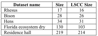
[image:8.612.327.517.378.448.2]

Table 1 lists the datasets in Group 1 (G1). Sizes of the datasets in this group ranges between 17 and 219 vertices.

Table 1: Group 1 (G1) Datasets

Dataset name Size LSCC Size

Rhesus 17 16

Bison 28 26

Hens 34 31

Florida ecosystem dry 130 103

Residence hall 219 214

Group 2 (G2) datasets are listed in Table 2. This group comprises 4 datasets with sizes between 1,006 and 2,941 vertices.

email-Eu-core 1,006 803

Blogs 1,226 793

UC Irvine messages 1,901 1,294

OpenFlights 2,941 2,868

The third group is Group 3 (G3) and contains 6 datasets with sizes between 12,647 and 220,972 vertices. G3 datasets are listed in Table 3.

Any Beat Dataset 12,647 8,518

FOLDOC 13,358 13,274

Edinburgh Associative

Thesaurus 23,134 7,751

BlogCatalog 88,786 88,784

Buzznet 101,170 95,470

(9)

4447 The last group is Group 4 (G4) with sizes

[image:9.612.127.517.463.729.2]

between 863,846 and 2,523,390 vertices. The datasets of G4 are listed in Table 4.

Wikipedia talk, Italian 863,846 36,356

Wikipedia talk, Arabic 1,095,799 8,797

Wikipedia talk, Chinese 1,219,243 10,831

Wikipedia talk, French 1,420,367 56,011

Hudong internal links 1,984,484 365,558

Flixster 2,523,390 99,803

The parameters settings for GWO are as follows:

 𝑎𝑔𝑒𝑛𝑡𝑠: we set this value to 5.

 𝑚𝑎𝑥𝐼𝑡𝑒𝑟𝑎𝑡𝑖𝑜𝑛𝑠: we set the value of this

parameter with respect to the group G1, G2, G3, and G4 to 2, 10, 32, and 128 respectively. We set to run each algorithm 30 times. Each time, we record the run time and solution, and calculate the solution quality and error rate. Then, the average run time, average solution quality, and average error rate are computed for each algorithm, they are listed in tables and figures for the purpose of comparisons.

4.2 Results and Discussions

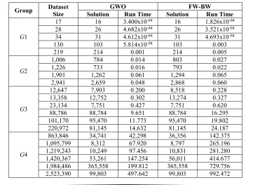
In Table 5, we record the run times and solutions obtained by both GWO and FW-BW.

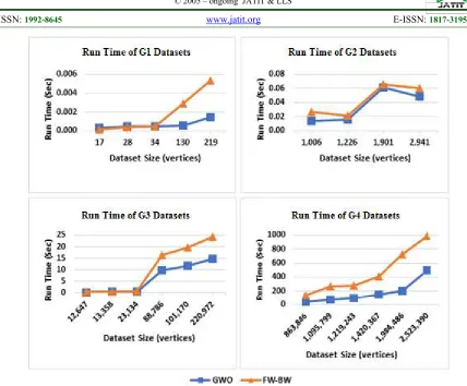
Then, we use the values in Table 5 to draw the run time curves shown in Figure 1.

In Figure 1, we show the run time comparison between GWO and FW-BW algorithms for all dataset groups (G1, G2, G3, and G4). Results show that GWO outperforms FW-BW in terms of run time for all groups.

As expected, GWO outperforms FW-BW due to the algorithm design of GWO. The heuristic nature of the GWO algorithm is the reason of the fast run times GWO algorithm achieved. According to the create_component() shown in Algorithm 3, random vertices are selected at each iteration of the function rather than all vertices that are descendent from the selected vertex as in the case of FW-BW algorithm. This reduces the run time dramatically especially as the size of the digraph grows.

On the other hand, when using the function

create_component() to create components, the selection of random vertices that are descendant from a given vertex rather than selecting all descending vertices causes some degradation to the solution quality, or accuracy, of the metaheuristic algorithm. Thus, solution quality (𝑠𝑞) is given in Definition 3.

Table 5: GWO vs FW-BW Solutions and Run Times (Seconds)

Group Dataset _Size _SolutionGWO _{Run Time} _SolutionFW-BW _{Run Time}

G1

17 16 3.400x10-04 ₁₆ _1.826x10-04

28 26 4.682x10-04 ₂₆ _3.521x10-04

34 31 4.612x10-04 ₃₁ _4.693x10-04

130 103 5.814x10-04 ₁₀₃ _0.003

219 214 0.001 214 0.005

G2

1,006 784 0.014 803 0.027

1,226 733 0.016 793 0.022

1,901 1,262 0.061 1,294 0.065

2,941 2,659 0.048 2,868 0.060

G3

12,647 7,903 0.200 8,518 0.228

13,358 12,752 0.302 13,274 0.327

23,134 7,751 0.427 7,751 0.620

88,786 88,784 9.651 88,784 16.295

101,170 95,470 11.773 95,470 19.802

220,972 81,145 14.632 81,145 24.187

G4

863,846 34,741 42.298 36,356 142.375

1,095,799 8,312 67.920 8,797 265.196

1,219,243 10,249 97.456 10,831 281.280

1,420,367 53,261 147.254 56,011 414.677

1,984,486 365,558 199.812 365,558 729.756

[image:9.612.127.498.466.730.2]

(10)

[image:10.612.93.521.60.414.2]

4448

Figure 1: Run Time Comparisons between GWO and FW-BW Algorithms Applied to Four Dataset Groups Definition 3. Solution Quality (𝒔𝒒) is a measure

of the correctness of the metaheuristic algorithm, and is measured as a ratio between the fitness value of the optimized solution (𝑓 ) and the value of the exact solution (𝑓 ) as shown in Equation (1).

𝑠𝑞 =𝑓

𝑓 (1)

We need also to compare the two algorithms, the metaheuristic and the exact one in terms of solution quality. In this context, let 𝑓 be the fitness value of the solution generated by GWO and 𝑓 be the fitness value of the solution generated by the FW-BW algorithms, then 𝑠𝑞 is the GWO solution quality which is given by Equation (2).

𝑠𝑞 = 𝑓

𝑓 (2)

The compliment of the solution quality is referred to as the error rate and is defined in Definition 4.

Definition 4. Error Rate (𝜼) is a measure of how far the solution given by the metaheuristic algorithm from that given by the exact algorithm, and is it computed as shown in Equation (3) as a compliment of the solution quality (𝑠𝑞).

𝜂 = 1 − 𝑠𝑞 (3)

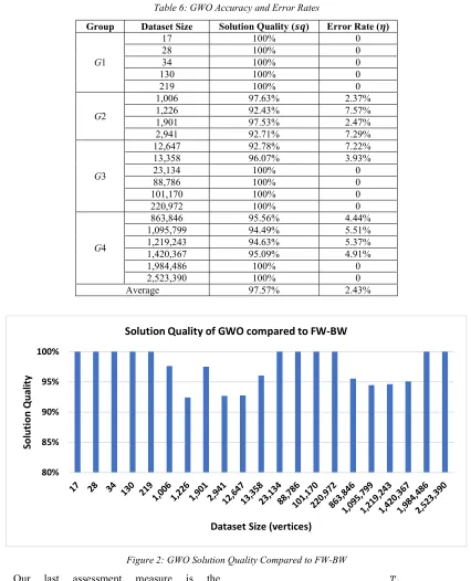
According to Equations (2) and (3) we calculate both the solution quality (𝑠𝑞) and the error rate (𝜂) and list them in Table 6. Then, in Figure 2 we depict the solution qualities for all datasets.

According to Table 6 and Figure 2, we can easily figure out that the minimum solution quality obtained by running the GWO algorithm on all datasets is more than 92%. On the other hand, the maximum error rate obtained is less than 8%.

(11)

[image:11.612.92.518.92.618.2]

4449

Table 6: GWO Accuracy and Error Rates

Group Dataset Size Solution Quality (𝒔𝒒) Error Rate (𝜼)

G1

17 100% 0

28 100% 0

34 100% 0

130 100% 0

219 100% 0

G2

1,006 97.63% 2.37%

1,226 92.43% 7.57%

1,901 97.53% 2.47%

2,941 92.71% 7.29%

G3

12,647 92.78% 7.22%

13,358 96.07% 3.93%

23,134 100% 0

88,786 100% 0

101,170 100% 0

220,972 100% 0

G4

863,846 95.56% 4.44%

1,095,799 94.49% 5.51%

1,219,243 94.63% 5.37%

1,420,367 95.09% 4.91%

1,984,486 100% 0

2,523,390 100% 0

Average 97.57% 2.43%

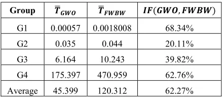
Figure 2: GWO Solution Quality Compared to FW-BW Our last assessment measure is the

improvement factor which is give in Definition 5. Definition 5. Run Time Improvement Factor (𝑰𝑭) is the percentage by which an algorithm has achieved enhancement over another algorithm. Let algorithms A and B be two algorithms with run times 𝑇 and 𝑇 respectively. The 𝐼𝐹 of Algorithm A over Algorithm B is given by equation (4).

𝐼𝐹(𝐴, 𝐵) = 1 −𝑇

𝑇 (4)

In Table 7, we calculate the average run time of each group of datasets for both GWO ( 𝑇 ) and FW-BW (𝑇 ). Then, we find the improvement factor for GWO over FW-BW

(𝐼𝐹(𝐺𝑊𝑂, 𝐹𝑊𝐵𝑊)).

80% 85% 90% 95% 100%

So

lu

tio

n

Q

ua

lit

y

(12)

[image:12.612.81.301.108.206.2]

4450 Table 7: Improvement Factors

Group 𝑻_𝑮𝑾𝑶 𝑻_{𝑭𝑾𝑩𝑾} 𝑰𝑭(𝑮𝑾𝑶, 𝑭𝑾𝑩𝑾)

G1 0.00057 0.0018008 68.34%

G2 0.035 0.044 20.11%

G3 6.164 10.243 39.82%

G4 175.397 470.959 62.76%

Average 45.399 120.312 62.27%

According to the results shown in Table 7, GWO achieved best improvement over FW-BW by more than 68% for G1 datasets.

In summary, the validity of research is proved internally and externally. Internal validity is proved by having results that comply to our asymptotic analysis which proved GWO to have a

O(𝑉 + 𝐸) run time complexity which is less than

the FW-BW O(𝑉𝐿𝑜𝑔𝑉) run time complexity. According to our experimental results, we were able to provide a metaheuristic solution to find the SCCs in digraphs using GWO in a reasonable time and solution quality compared to the FW-BW exact method. On average, GWO achieves 62.27% improvement over FW-BW. On the other hand, external validity of the research is proved by applying the GWO algorithms to different datasets from different sources which represent different real-world graphs.

5. CONCLUSIONS AND FUTURE WORK

In this paper, we introduced a metaheuristic algorithm to find SCCs in digraphs using the Grey Wolf Optimizer (GWO). First, the worst-case run time complexity of the GWO algorithm is shown and proved asymptotically to be O(𝑉 + 𝐸). Then, we set the GWO algorithm to run against a number of datasets downloaded from different benchmarks used frequently in research. We also implemented a well-known algorithm, which is the FW-BW algorithm. Experimental results show that GWO outperformed FW-BW in terms of run time. This conforms to the asymptotic run time complexity which is proved to be linear for GWO and

O(𝑉𝐿𝑜𝑔𝑉) for the FW-BW algorithm. It is also

related to the algorithmic design of both algorithms. Since FW-BW uses the divide-and-conquer approach to find exact solutions, GWO uses metaheuristics to find near-optimal solutions attempting to compromise solution accuracy in favor of run time. In this context, results also show that the average solution quality for the GWO

algorithm was 97.57%. Also, GWO achieved 62.27% average run time improvement over FW-BW.

As a future work, more metaheuristic algorithms can be designed to find SCCs in digraphs and compare to GWO or FW-BW. Also, GWO can also be parallelized and compared to the sequential GWO. In this context, the problem can be implemented in parallel using different interconnection networks such as: the hypercube, mesh, Chained-Cubic Tree (CCT) [40], as well as optoelectronic interconnection networks such as: the OTIS-Hypercube, OTIS-Mesh, OTIS Hyper Hexa-Cell, or Optical Chained-Cubic Tree (OCCT) interconnection networks [16] [41] [42].

REFERENCES:

[1] S. Dhingra, P. S. Dodwad and M. Madan, "Finding Strongly Connected Components in a Social Network Graph," International Journal of Computer Applications, vol. 136, no. 7, pp. 1-5, 2016.

[2] L. K. Fleischer, B. Hendrickson and A. Pınar, "On Identifying Strongly Connected Components in Parallel," in International Parallel and Distributed Processing Symposium. IPDPS 2000. Parallel and Distributed Processing, vol. 1800, J. Rolim, Ed., Berlin, Heidelberg, Springer, 2000, pp. 505-511.

[3] K. H. Rosen, Discrete Mathematics and Its Applications, 7th ed., McGraw-Hill Education, 2011.

[4] Y. L. Traon, T. Jéron, J.-M. Jézéquel and P. Morel, "Efficient Object-Oriented Integration and Regression Testing," IEEE Transactions on Reliability, vol. 49, no. 1, pp. 12-25, 2000.

[5] J. Jeong and P. Berman, "On cycles in the transcription network of Saccharomyces cerevisiae," BMC Systems Biology, vol. 2, no. 1, p. 12, 2008.

[6] R. Tarjan, "Depth-First Search and Linear Graph Algorithms," SIAM Journal on Computing, vol. 1, no. 2, p. 146–160, 1972. [7] J. H. Reif, "Depth-first search is inherently sequential," Information Processing Letters, vol. 20, no. 5, pp. 229-234, 1985.

(13)

4451 International Journal of Advanced Computer Science and Applications (IJACSA), vol. 7, no. 6, pp. 336-342, 2016. [9] A. Shaheen, A. Sleit and S. Al-Sharaeh, "A

Solution for Traveling Salesman Problem using Grey Wolf Optimizer Algorithm," Journal of Theoretical and Applied Information Technology, vol. 96, no. 18, pp. 6256-6266, 2018.

[10] E.-G. Talbi, Metaheuristics from Design to Implementation, Wiley, 2009.

[11] S. Hong, N. C. Rodia and K. Olukotun, "On fast parallel detection of strongly connected components (SCC) in small-world graphs," in SC '13 Proceedings of the International Conference on High Performance Computing, Networking, Storage and Analysis, Denver, Colorado, 2013.

[12] W. McLendon III, B. Hendrickson, S. J. Plimpton and L. Rauchwerger, "Finding strongly connected components in distributed graphs," Journal of Parallel and Distributed Computing, vol. 65, no. 8, pp. 901-910, 2005.

[13] D. J. Pearce, "A space-efficient algorithm for finding strongly connected components," Information Processing Letters, vol. 116, no. 1, pp. 47-52, 2016.

[14] A. Al-Shaikh, R. Al-Sayyed and A. Sleit, "A Case Study for Evaluating Facebook Pages with Respect to Arab Mainstream News Media," Jordanian Journal of Computers and Information Technology, vol. 3, no. 3, pp. 142-156, 2017.

[15] K. Sörensen and F. W. Glover, "Metaheuristics," in Encyclopedia of Operations Research and Management Science, S. I. Gass and M. C. Fu, Eds., Springer US, 2013, pp. 960-970.

[16] A. Al-Adwan, A. Sharieh and B. A. Mahafzah, "Parallel heuristic local search algorithm on OTIS hyper hexa-cell and OTIS mesh of trees optoelectronic architectures," Applied Intelligence, 2018. [17] B. A. Mahafzah, "Performance Evaluation

of Parallel Multithreaded A* Heuristic Search Algorithm," Journal of Information Science, vol. 40, no. 3, pp. 363-375, 2014. [18] B. A. Mahafzah, "Parallel Multithreaded

IDA* Heuristic Search: Algorithm Design and Performance Evaluation," International

Journal of Parallel, Emergent and Distributed Systems, vol. 26, no. 1, p. 61–82, 2011.

[19] I. Boussaïd, J. Lepagnot and P. Siarry, "A survey on optimization metaheuristics," Information Sciences, vol. 237, pp. 82-117, 2012.

[20] L. Pigatto, M. Baruzzo, P. Bettini, T. Bolzonella, G. Manduchi, G. Marchiori and F. Villone, "Control System Optimization Techniques for Real-Time Applications in Fusion Plasmas: The RFX-mod Experience," IEEE Transactions on Nuclear Science, vol. 64, no. 6, pp. 1420-1425, 2017. [21] Z. Wang, K. Droegemeier and L. White, "The Adjoint Newton Algorithm for Large-Scale Unconstrained Optimization in Meteorology Applications," Computational Optimization and Applications, vol. 10, no. 3, pp. 283-320, 1998.

[22] A. Al-Shaikh and A. Sleit, "Evaluating IndexedDB performance on web browsers," in 2017 8th International Conference on Information Technology (ICIT), Amman, Jordan , 2017.

[23] M. Alshraideh, B. A. Mahafzah and S. Al-Sharaeh, "A multiple-population genetic algorithm for branch coverage test data generation," Software Quality Journal, vol. 19, no. 3, pp. 489-513, 2011.

[24] M. Alshraideh, E. Jawabreh, B. A. Mahafzah and H. M. A. Harahsheh, "Applying Genetic Algorithms to Test JUH DBs Exceptions," International Journal of Advanced Computer Science and Applications, vol. 4, no. 7, pp. 8-20, 2013.

[25] M. A. Alshraideh, B. A. Mahafzah, H. S. E. Salman and I. Salah, "Using genetic algorithm as test data generator for stored PL/SQL program units," Journal of Software Engineering and Applications, vol. 6, no. 2, pp. 65-73, 2013.

[26] S. Mirjalili, S. M. Mirjalili and A. Lewis, "Grey Wolf Optimizer," Advances in Engineering Software, vol. 69, pp. 46-61, 2014.

(14)

4452 [28] A. Hudaib, R. Masadeh and A. Alzaqebah,

"WGW: A Hybrid Approach Based on Whale and Grey Wolf Optimization Algorithms for Requirements Prioritization," Advances in Systems Science and Applications, vol. 18, no. 2, pp. 63-83, 2018.

[29] R. Masadeh, A. Sharieh and A. Sleit, "Grey wolf optimization applied to the maximum flow problem," International Journal of Advanced and Applied Sciences, vol. 4, no. 7, pp. 95-100, 2017.

[30] A. Al-Shaikh, H. Khattab and S. Al-Sharaeh, "Performance Comparison of LEACH and LEACH-C Protocols in Wireless Sensor Networks," Journal of ICT Research and Applications, vol. 12, no. 3, pp. 219-236, 2018.

[31] R. Rajakumar, J. Amudhavel, P. Dhavachelvan and T. Vengattaraman, "GWO-LPWSN: Grey Wolf Optimization Algorithm for Node Localization Problem in Wireless Sensor Networks," Journal of Computer Networks and Communications, vol. 2017, p. 10, 2017.

[32] N. A. Al-Aboody and H. S. Al-Raweshidy, "Grey wolf optimization-based energy-efficient routing protocol for heterogeneous wireless sensor networks," in 2016 4th International Symposium on Computational and Business Intelligence (ISCBI), Olten, Switzerland, 2016.

[33] C. S. Shieh, T. T. Nguyen, H. Y. Wang and T. K. Dao, "Enhanced Diversity Herds Grey Wolf Optimizer for Optimal Area Coverage in Wireless Sensor Networks," in Genetic and Evolutionary Computing, J. Pan, J. C. Lin, C. Wang and X. H. Jiang, Eds., Springer International Publishing, 2017, pp. 174-182. [34] M. Sharawi and E. Emary, "Impact of grey wolf optimization on WSN cluster formation and lifetime expansion," in 2017 Ninth International Conference on Advanced Computational Intelligence (ICACI), Doha, Qatar, 2017.

[35] T. S. Murugan and A. Sarkar, "Optimal cluster head selection by hybridisation of firefly and grey wolf optimisation," International Journal of Wireless and Mobile Computing, vol. 14, no. 3, pp. 296-305, 2018.

[36] J. Kunegis, " KONECT - The Koblenz Network Collection," in Int. Web Observatory Workshop, 2013.

[37] J. Leskovec and R. Sosic, "SNAP: A General-Purpose Network Analysis and Graph-Mining Library," ACM Transactions on Intelligent Systems and Technology (TIST), vol. 8, no. 1, p. 1, 2016.

[38] M. Fire, R. Puzis and Y. Elovici, "Link Prediction in Highly Fractional Data Sets," Handbook of Computational Approaches to Counterterrorism, 2012.

[39] R. Zafarani and H. Liu, "Social Computing Data Repository at {ASU}," 2009.

[40] M. Abdullah, E. Abuelrub and B. A. Mahafzah, "The chained-cubic tree interconnection network," International Arab Journal of Information Technology, vol. 8, no. 3, pp. 334-343, 2011.

[41] B. A. Mahafzah, M. Alshraideh, T. M. Abu-Kabeer, E. F. Ahmad and N. A. Hamad, "The optical chained-cubic tree interconnection network: Topological structure and properties," Computers & Electrical Engineering, vol. 38, no. 2, pp. 330-345, 2012.