A stochastic model for the evolution of the web allowing link deletion

(1)

BIROn - Birkbeck Institutional Research Online

Fenner, Trevor and Levene, Mark and Loizou, George (2006) A stochastic

model for the evolution of the web allowing link deletion. ACM Transactions

on Internet Technology 6 (2), pp. 117-130. ISSN 1533-5399.

Downloaded from:

Usage Guidelines:

Please refer to usage guidelines at or alternatively

(2)

Birkbeck ePrints: an open access repository of the

research output of Birkbeck College

http://eprints.bbk.ac.uk

Fenner, Trevor; Levene, Mark; and Loizou, George (200

6 )

A stochastic model for the evolution of the web allowing

link deletion

.

ACM Transactions in Internet Technology

6 (2)

117-130

This is an author-produced version of a paper to be published in

ACM

Transactions in Internet Technology

(ISSN 1533-5399). This version has been

peer-reviewed but does not include the final publisher proof corrections,

published layout or pagination.

All articles available through Birkbeck ePrints are protected by intellectual

property law, including copyright law. Any use made of the contents should

comply with the relevant law.

Citation for this version:

Fenner, Trevor; Levene, Mark; and Loizou, George (2006)

A stochastic model

for the evolution of the web allowing link deletion

.

London: Birkbeck ePrints.

Available at: http://eprints.bbk.ac.uk/archive/00000268

Citation for the publisher’s version:

Fenner, Trevor; Levene, Mark; and Loizou, George (2006)

A stochastic model

for the evolution of the web allowing link deletion

.

ACM Transactions in

Internet Technology

6 (2) 117-130

.

http://eprints.bbk.ac.uk

(3)

arXiv:cond-mat/0304316 v2 25 Mar 2004

A Stochastic Model for the Evolution of the Web

Allowing Link Deletion

Trevor Fenner, Mark Levene, and George Loizou School of Computer Science and Information Systems

Birkbeck College, University of London London WC1E 7HX, U.K.

{trevor,mark,george}@dcs.bbk.ac.uk

Abstract

Recently several authors have proposed stochastic evolutionary models for the growth of the web graph and other networks that give rise to power-law distributions. These models are based on the notion of preferential attachment leading to the “rich get richer” phenomenon. We present a generalisation of the basic model by allowing deletion of individual links and show that it also gives rise to a power-law distribution. We derive the mean-field equations for this stochastic model and show that, by examining a snapshot of the distribution at the steady state of the model, we are able to tell whether any link deletion has taken place and estimate the probability of deleting a link. Applying our model to actual web graph data gives some insight into the distribution of inlinks in the web graph and provides evidence of link deletion and the extent to which this has occurred. Our analysis of the data also suggests a power-law exponent of approximately 2.15 rather than the widely published value of 2.1.

1 Introduction

Power-law distributions taking the form

f(i) =C i−τ_, ₍₁₎

where C and τ are positive constants, are abundant in nature [Sch91]. The constant τ is

called theexponent of the distribution. Examples of such distributions are: Zipf ’s law, which

states that the relative frequency of words in a text is inversely proportional to their rank,

Pareto’s law, which states that the number of people whose personal income is above a certain

level follows a power-law distribution with an exponent between 1.5 and 2,Lotka’s law, which

states that the number of authors publishing a prescribed number of papers is inversely

proportional to the square of the number of publications, andGutenberg-Richter’s law, which

states that the number of earthquakes over a period of time having a certain magnitude is roughly inversely proportional to the magnitude.

Recently several researchers have detected asymptotic power-law distributions in the

topology of the World-Wide-Web [BKM+_{00, DKM}+_{02] and, in parallel, researchers from}

(4)

the web and other networks such as the internet, citation networks, collaboration networks

and biological networks. A common theme in these models is that ofpreferential attachment,

which results in the “rich get richer” phenomenon, for example, when new links to web pages are added in proportion to the number of currently existing links to these pages. Related ap-proaches are the general theoretical model covering both directed and undirected web graphs [CF03], the stochastic multiplicative process in which nodes appear at different times and the rate of addition of links varies between nodes [AH01], and the statistical physics approach that uses the rate equation technique [KR02].

To explain situations where pure preferential attachment models fail, we [LFLW02] and

others [PFL+_{02] have previously proposed extensions of the stochastic model for the web’s}

evolution in which the addition of links is prescribed by a mixture of preferential and non-preferential mechanisms. In [LFLW02], we devised a general stochastic model involving the transfer of balls between urns; this also naturally models quantities such as the numbers of web pages in and visitors to a web site, which are not naturally described in graph-theoretic terms. We note that our urn model is an extension of the stochastic model proposed by Simon in his visionary paper published in 1955 [Sim55], which was couched in terms of word frequencies in a text. We also considered an alternative extension of Simon’s model in [FLL02] by adding a preferential mechanism for discarding balls from urns (corresponding to deleting web pages); this results in an exponential cutoff in the power-law distribution.

Our urn transfer model is a stochastic process, in which at each step with probabilityp a

new ball (which might represent a web page) is added to the first urn and with probability

1−p a ball in some urn is moved along to the next urn. We assume that a ball in theith urn

hasipins attached to it (which might represent web links). It is known that the steady-state

distribution of this model is a power law, with exponentτ = 1 + 1/(1−p) [Sim55, LFLW02].

As mentioned above, the power-law distribution breaks down when balls may be discarded, resulting in a power-law distribution with an exponential cutoff. So the question arises as to whether it also breaks down when removal of pins is allowed. We answer this question here by showing that the power-law distribution does not break down, under the constraint that more balls are added to the system than are removed. (When the only remaining pin is removed from a ball in the first urn that ball is removed from the system.) This model gives a more realistic explanation for the emergence of power laws in complex networks than the basic model without link deletion (i.e. pin removal). Considering, for example, the web graph, the modification we make to the basic model is that after a web page is chosen preferentially, say according to the number of its inlinks, there is a small probability that some link to this page will be deleted. (This is equivalent to deleting a link chosen uniformly at random.) A possible reason for this may be that popular web pages compete for inlinks, so that the number of inlinks a page has acquired will fluctuate with its popularity. This is evident, for example, in the rise and fall in the popularity of several search engines. Link deletion has also been considered by Dorogovtsev and Mendes [DM01] in the context of a different model in which, at each time step, a new node is added with just one link, which preferentially attaches

itself to an existing node. In addition, at each time step m links between existing nodes are

added to preferentially chosen nodes and c links between existing nodes are deleted, again

preferentially. Their conclusion that link deletion increases the power-law exponent is also obtained here for our stochastic model.

Consider a power law such as Lotka’s law [Nic89]. If this holds, then a plot on a log-log

(5)

should reveal a straight line with a negative slope of around−2. There is an obvious problem with a log-log transformation if any of the frequencies are zero; that is to say, when there

are values v1 and v2, with v1< v2, for whichnoauthor published v1 papers but at least one

author published v2 papers (i.e. there is agap in the values for the number of publications).

In general, we expect such gaps to occur in any data set, mainly for large values. (This is due to the stochastic variation and the fact that the frequencies have to be integral.) This observation is consistent with the finding that Lotka’s law does not fit well for large values (i.e. authors who published a large number of papers) and this tail region is characterised by the presence of gaps [Nic89].

One way of dealing with the problem of gaps is simply to ignore all value-frequency pairs where the frequency is zero. However, ignoring gaps in this way seems questionable, since the zero frequency values do give relevant information about the data set and should not be treated as missing values. Our unease with this approach is reinforced by the fact that computing the exponent in this way results in a much lower value; for example, for the web

inlink data [BKM+00], it gives a value around 1.5, rather than the generally accepted figure

of 2.1.

An alternative approach is to squash the non-zero frequencies up towards the y-axis (i.e. the frequency axis), after ignoring the zero frequency values. This is equivalent to omitting from the data set those values for which there are no authors having that number of pub-lications and then ranking the remaining values in increasing order, i.e. renumbering the values starting from one. This method also seems somewhat dubious, since the power-law relationship should really involve the actual values rather than their ranks.

The standard technique for fitting a power-law distribution uses linear regression on log-log transformed data, which is not possible if gaps are present. Another approach for handling gaps is to consider only the values up until the first gap; this approach is only reasonable

if the first gap does not occur at too low a value. We call this theunranked approach, and

note that this approach ignores the large values in the tail of the distribution. The unranked approach suggests one possible solution, but other approaches, such as smoothing or using theHill plot [DdR00], are possible. Ad-hoc approaches have the disadvantage that they are hard to justify, and the Hill plot, as originally defined, is only applicable after the data has been sorted, and this also seems difficult to justify.

Another solution for handling gaps is the second method described above of ranking the

values with non-zero frequencies and squashing up; we call this the ranked approach. In

general, we should not expect the ranked and unranked approaches to yield the same power-law exponent. We would expect the exponent computed by linear regression on the log-log transformed data from the unranked approach to be somewhat higher. One of the findings of this paper is that for inlinks in the web graph the ranked and unranked approaches lead to a small but noticeable difference between the exponents. (Our previous comments indicate why we have misgivings with the ranked approach.)

(6)

probability. In Section 5 we utilise our urn model to describe a discrete stochastic process that simulates the evolution of the degree distribution of inlinks in the web graph. As a proof

of concept, we analyse the May 1999 data set for inlinks presented in [BKM+00], which we

obtained from Ravi Kumar at IBM. We are able to show that our model is consistent with the data and determine the extent to which link deletion has occurred. We also investigate the discrepancy between the ranked and unranked approaches. With the ranked approach,

using linear regression on the log-log transformed data, an exponent of 2.1 is obtained, as in

[BKM+00]. However, the unranked approach results in an exponent of 2.15, which is shown

to be consistent with our stochastic model. Although the difference between 2.1 and 2.15 may

not seem significant, it has been remarked in [BKM+_{00] that “2.1 is in remarkable agreement}

with earlier studies” and in [DKM+02] that the exponent is “reliably around 2.1 (with little

variation)”, which justifies us in making a distinction between the exponents obtained using the ranked and unranked approaches. Finally, in Section 6 we give our concluding remarks.

2 An Urn Transfer Model

We now present an urn transfer model for a stochastic process with urns containing balls

(which might represent web pages) that have pins (which might represent either inlinks or outlinks) attached to them. Our model allows for pins to be discarded with a small probability. This model can be viewed as an extension of Simon’s model [Sim55]. We note that there is

a correspondence between the Barab´asi and Albert model [BA99], defined in terms of nodes

and links, and Simon’s model, defined in terms of balls and pins, as was established in [BE01]. Essentially, the correspondence is obtained by noting that the balls in an urn can be viewed as an equivalence class of nodes all having the same indegree (or outdegree).

We assume a countable number of urns, urn1, urn2, urn3, . . . , where each ball inurni is

assumed to haveipins attached to it. Initially all the urns are empty excepturn1, which has

one ball in it. LetFi(k) be the number of balls inurni at stage kof the stochastic process,

soF1(1) = 1. Then, for k≥1, at stagek+ 1 of the stochastic process one of two things may

occur:

(i) with probabilityp, 0< p <1, a new ball is inserted into urn1, or

(ii) with probability 1 −p an urn is selected, with urni being selected with probability

proportional to iFi(k), and a ball is chosen fromurni; then,

(a) with probability r, 0 < r ≤ 1, the chosen ball is transferred to urni+1, (this is

equivalent to attaching an additional pin to the ball chosen from urni), or

(b) with probability 1−r, the ball is transferred tourni−1 ifi >1, otherwise, ifi= 1,

the ball is discarded (this is equivalent to removing and discarding a pin from the

ball chosen fromurni).

In the special case whenr= 1, the process reduces to Simon’s original model.

We note that choosing a ball preferentially (in proportion to the number of pins) is equiv-alent to selecting a pin uniformly at random and choosing the ball it is attached to. Thus,

(7)

Since iFi(k) is the total number of pins attached to balls in urni, the expected total

number of pins in the urns at stagek is given by

E

k

X

i=1

iFi(k)

= 1 + (k−1) (p+ (1−p)r−(1−p)(1−r))

= 1 + (k−1) (1−2(1−p)(1−r)). (2)

Correspondingly, the expected total number of balls in the urns is given by

E

k

X

i=1

Fi(k)

= 1 + (k−1)p−(1−p)(1−r)

k−1

X

j=1

φj, (3)

where φj, 1 ≤ j ≤ k−1, is the expected probability of choosing urn1 at step (ii) of stage

j+ 1, i.e.

φj =E

F1(j)

Pj

i=1iFi(j)

!

. (4)

Now let

φ(k)= 1

k

X

j=1

φj. (5)

In order to ensure that there are at least as many pins in the system as there are balls and that, on average, more balls are added to the system than are removed, we require the following constraint, derived from (2) and (3),

1−2r

1−r ≤φ

(k)_≤ p

(1−p)(1−r). (6)

This implies

2(1−p)(1−r)≤1, (7)

which obviously holds forr≥1/2. Inequality (7) expresses the fact that the expected number

of pins should not be negative, and follows from (2).

We note that we could modify the initial conditions so that, for example, urn1 initially

containedδballs,δ >1, instead of just one ball. It can be shown, from the development of the

model below, that any change in the initial conditions will have no effect on the asymptotic

distribution of the balls in the urns as k tends to infinity, provided the process does not

terminate with all of the urns empty. More specifically, the probability that the process will not terminate with all the urns empty is given by

1−

₍₁₋_p₎₍₁₋_r₎

1−(1−p)(1−r)

δ

. (8)

This is exactly the probability that the gambler’s fortune will increase forever [Ros83].

(We note that (8) only makes sense if (7) holds.) Since, in practice, r will be quite close to

(8)

3 Derivation of the Steady State Distribution

Following Simon [Sim55], we now state the mean-field equations for the urn transfer model.

Fori >1 the expected number of balls in urni is given by

Ek(Fi(k+ 1)) =Fi(k) +βk

r(i−1)Fi−1(k) + (1−r)(i+ 1)Fi+1(k)−iFi(k)

, (9)

whereEk(Fi(k+ 1)) is the expected value ofFi(k+ 1), given the state of the model at stage

k, and

βk=

1−p

Pk

i=1 iFi(k)

(10)

is the required normalising factor.

In the boundary case, wheni= 1, we have

Ek(F1(k+ 1)) =F1(k) +p+βk

(1−r) 2F2(k)−F1(k)

, (11)

for the expected number of balls inurn1, given the state at stage k.

In order to obtain a solution for the model, we assume that, for large k, the random

variableβkcan be approximated by a constant value ˆβk depending only onk. This is defined

by

ˆ

βk=

1−p

k(1−2(1−p)(1−r)).

The motivation for this approximation is that the denominator in the definition ofβk, the

total number of pins, has been replaced by its expectation given in (2). This is a reasonable assumption since the number of pins is the difference between two binomial random variables,

and with high probability this will be close to its expected value. We observe that using ˆβk

as the normalising factor instead of βk results in an approximation similar to that of the “pk

model” in [LFLW02].

Replacing βk by ˆβk and taking the expectations of (9) and (11), we obtain

E(Fi(k+1)) =E(Fi(k))+ ˆβk

r(i−1)E(Fi−1(k))+(1−r)(i+1)E(Fi+1(k))−iE(Fi(k))

(12)

and

E(F1(k+ 1)) =E(F1(k)) +p+ ˆβk

(1−r) 2E(F2(k))−E(F1(k))

, (13)

respectively.

In order to solve (12) and (13), we would like to show that E(Fi(k))/k tends to a limit

fi as k tends to infinity. Suppose for the moment that this is the case, then, provided the

convergence is fast enough, E(Fi(k+ 1))−E(Fi(k)) tends tofi. By “fast enough” we mean

that ǫi,k+1−ǫi,k iso(1/k) for largek, where

(9)

Now, letting

β=kβˆk=

1−p

1−2(1−p)(1−r), (14)

we see that ˆβkE(Fi(k)) tends to βfi asktends to infinity. Thus, letting ktend to infinity in

(12) and (13), these yield

fi=β

r(i−1)fi−1+ (1−r)(i+ 1)fi+1−ifi

, (15)

and

f1=p+β

(1−r)2f2−f1

, (16)

respectively.

We now investigate the asymptotic behaviour of fi for large i. If we define gi to be ifi,

we can rewrite (15) and (16) as

rgi−1

gi

+(1−r)gi+1

gi

= 1 + 1

iβ (17)

and

p

βg1

+ (1−r)g2

g1

= 1 + 1

β. (18)

Suppose we can writegi as

gi =

C Γ(i+α+ 1)

Γ(i+α+ 1 +ρ)

1 + η

i2 +O

₁

i3

, (19)

where α,η,ρ and C are constants.

Using the binomial theorem and the fact that Γ(x+ 1) =xΓ(x), we get

gi−1

gi

≈ i+α+ρ

i+α

1 + η

i2 +O

₁

i3 1−

η

i2 +O

₁

i3

= i+α+ρ

i+α

1 +O

₁

i3

= 1 + ρ

i −

ρα

i2 +O

₁

i3

. (20)

Similarly,

gi+1

gi

≈ i+α+ 1

i+α+ρ+ 1

1 +O

₁

i3

= 1−ρ

i +

ρ(α+ρ+ 1)

i2 +O

₁

i3

. (21)

Substituting (20) and (21) into the left-hand side of (17), we obtain

r

1 +ρ

i −

ρα

i2 +O

₁

i3

+ (1−r)

1− ρ

i +

ρ(α+ρ+ 1)

i2 +O

₁

i3

= 1 + 1

(10)

which simplifies to

1 +ρ

i(2r−1) +

ρ

i2

(1−r)(ρ+ 1)−(2r−1)α+O

₁

i3

= 1 + 1

iβ. (22)

For this to hold for all large enough values ofi, we require

ρ= 1

β(2r−1), (23)

and

α= (1−r)(ρ+ 1)

2r−1 . (24)

It is straightforward to obtain more terms in the expansion of (19) by a more detailed analysis, for example

η= ρ (1−r)(α+ρ+ 1)

2₋_rα2

2(2r−1) .

So, with ρ and α as in (23) and (24), for large i, (19) gives an approximate solution to

the recurrence defined by (15) and (16). Thus,

fi∼C i−(1+ρ), (25)

where C is independent of iand ∼meansis asymptotic to.

From (23) and (14),

ρ= 1 +

_p

1−p

1

2r−1

. (26)

If, as is usually the case, we assume thatρ is positive, then r > 1/2, and it follows that

increasingpincreasesρ, whereas increasingrdecreases ρ. In particular, we observe from (26)

that with pin removal, i.e. forr <1, the exponent of the power law is greater than it would

be forr= 1, i.e.

ρ≥ 1

1−p. (27)

4 Recognising Pin Removal

In this section we show that, using the mean-field equations derived in Section 3, we are able to detect whether pin removal has taken place by inspecting a static snapshot of the system at the steady state.

Based on (2) and (3) we have

pins

(11)

balls

k ≈p−(1−p)(1−r)φ, (29)

where pins and balls stand for the expected numbers of pins and balls at stage k, and φ is

the asymptotic value ofφ(k)_{, defined by (5), i.e. the expected proportion of pins in the first}

urn, |urn1|/pins. The right-hand sides of (28) and (29) give asymptotic values of pins and

ballsasktends to infinity. It follows that the asymptotic value of the ratioballs/pins, which

we denote by ∆, is given by

∆ = p−(1−p)(1−r)φ

1−2(1−p)(1−r). (30)

From this and the fact that ∆≥φ, it follows that

φ≤ p

1−(1−p)(1−r) ≤∆≤

p

1−2(1−p)(1−r). (31)

Using (7) and (26), this implies

φ

2 ≤p≤∆≤

ρ−1

ρ . (32)

Now suppose we are givenρ, ∆ andφ. Then from (26) and (30) we can derive the following

equations:

p= φ(ρ−1)

2ρ(1−∆)−2 +ρφ, (33)

r= 1

2

1 + φ

2ρ(1−∆)−2 +φ

. (34)

Now suppose we observe an urn process with 1/2< r ≤1 and 0< p <1, and we take a

snapshot of the system at the steady state, obtaining empirical estimates forρ, ∆ andφfrom

the distribution of the balls in the urns. We would like to check whether it is possible that

these values could have arisen from Simon’s process, i.e. withr = 1, with the probability of

inserting a ball into the first urn equal to, say, p′_{. So from (26) and (30) we would require}

ρ= 1/(1−p′_{) and ∆ =}_p′_{. Thus, from (26), we would obtain}

p′₌ ρ−1

ρ =

p

1−2(1−p)(1−r), (35)

and, from (30),

p′_{= ∆ =} p−(1−p)(1−r)φ

1−2(1−p)(1−r). (36)

It is evident that (35) and (36) can only be consistent if r≈1. Thus, simulating the urn

process with p′ _{= (}_ρ₋₁₎_/ρ _and _r_{= 1 would result in the same value for} _ρ _{as that obtained}

frompand the original value ofr. However, in the presence of pin removal, the value of ∆ (i.e.

the asymptotic value ofballs/pins) would be less than p′_{, the probability of inserting a new}

ball into the first urn. This provides a discriminator between the two processes. As a result, by examining the said snapshot we are able to ascertain whether the process is consistent

with the urn model in which pins may be discarded, i.e. withr <1. We apply this analysis

(12)

5 A Model for the Evolution of the Web Graph

We now describe a discrete stochastic process for simulating the evolution of the degree distribution of inlinks in the web graph. In this model, balls correspond to web pages and pins correspond to inlinks. At each time step the state of the web graph is a directed graph

G = (N, E), where N is its node set and E is its arc set. In this scenario Fi(k), i ≥ 1, is

the number of pages (nodes) in the web graph having iinlinks. We note that, although we

have chosen i to denote the number of inlinks, i could alternatively denote the number of

outlinks, the number of pages in a web site, or any other reasonable parameter we would like to investigate; see [LFLW02] for further details.

Consider the evolution of the web graph with respect to the number of pages having i

inlinks at thekth step of the process. InitiallyGcontains just a single page. At each step one

of three things can happen. First, with probabilityp a new page having one incoming link is

added to G; this is equivalent to placing a new ball in urn1. Alternatively, with probability

1−p a page is chosen, the probability of choosing a given page being proportional to i, the

number of inlinks the page currently has; this is equivalent to preferentially choosing a ball

from urni. Then, with probabilityr the chosen page receives a new inlink; this is equivalent

to transferring the chosen ball from urni to urni+1. Alternatively, with probability 1−r an

inlink to the page is removed, and if the page has no inlinks remaining it is removed from

the graph; this is equivalent to transferring the ball tourni−1 wheni >1, and discarding the

ball from the system ifi= 1.

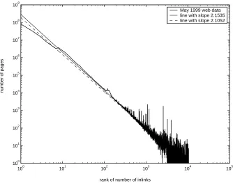
As a proof of concept, we use the inlinks data from a large crawl of the web performed

during May 1999 [BKM+00]; the data set we used in this analysis was obtained from Ravi

Kumar at IBM. After removing web pages with zero inlinks from the data set, there remain approximately 177 million pages with a total of 1.466 billion inlinks. Using the ranked

ap-proach, linear regression on the log-log transformed data gives an exponent of 2.1052, which is

consistent with the value of 2.1 reported in [BKM+_{00] and confirmed subsequently in [AB02];}

6 Concluding Remarks

We have presented an extension of Simon’s classical stochastic process that allows for pins (which might represent web links) to be discarded, and have shown that asymptotically it still follows a power-law distribution. Given a snapshot of a system, the mean-field equations

that we have derived give estimates of the parametersp and r, which can then be input to

our stochastic process simulating the evolution of the system. We applied our analysis to the

May 1999 web crawl data [BKM+00] to detect the extent to which link deletion had taken

place. The values of p and r that we have obtained indicate that approximately 15% of all

link operations are deletions. We also ran a number of simulations to validate the mean-field analysis.

An interesting finding that came to light when analysing the data was that there is good

evidence that the exponent of the power law for inlinks is in fact close to 2.15 rather than

to the widely published value of 2.1. Although the difference between these exponents is

small, we consider it to be significant because it suggests a more justifiable way to use linear regression to obtain exponents from power law data.

It would be interesting to study link deletion through historical data, such as that provided

by the wayback machine [Not02] (http://www.waybackmachine.org), in order to gain more

insight into the dynamic aspects of the evolution of the web graph. In particular, it would

be desirable to determine whether and how the exponent, and the parameters p and r, are

changing over time.

Acknowledgements. The authors would like to thank Ravi Kumar at IBM for providing us with the inlinks data set. We would also like to thank the referees for their constructive comments, which have helped us to improve the presentation of the results.

References

[AB02] R. Albert and A.-L. Barab´asi. Statistical mechanics of complex networks. Reviews

(15)

[AH01] L.A. Adamic and B.A. Huberman. The Web’s hidden order. Communications of the ACM, 44(9):55–59, 2001.

[BA99] A.-L. Barab´asi and R. Albert. Emergence of scaling in random networks. Science,

286:509–512, 1999.

[BE01] S. Bornholdt and H. Ebel. World Wide Web scaling exponent from Simon’s 1955

model. Physical Review E, 64:035103–1–035104–4, 2001.

[BKM+00] A. Broder, R. Kumar, F. Maghoul, P. Raghavan, A. Rajagopalan, R. Stata,

A. Tomkins, and J. Wiener. Graph structure in the Web. Computer Networks,

33:309–320, 2000.

[CF03] C. Cooper and A.M. Frieze. A general model of web graphs. Random Structures

and Algorithms, 22:311–335, 2003.

[DdR00] H. Drees, L. de Haan, and S. Resnick. How to make a Hill plot. Annals of

Statistics, 28:254–274, 2000.

[DKM+_{02] S. Dill, R. Kumar, K. McCurley, S. Rajagopalan, D. Sivakumar, and A. Tomkins.}

Self-similarity in the web. ACM Transactions on Internet Technology, 2:205–223,

2002.

[DM01] S.N. Dorogovtsev and J.F.F. Mendes. Scaling properties of scale-free evolving

networks: Continuous approach. Physical Review E, 35:056125, 2001.

[DM02] S.N. Dorogovtsev and J.F.F. Mendes. Evolution of networks.Advances in Physics,

51:1079–1187, 2002.

[FLL02] T.I. Fenner, M. Levene, and G. Loizou. A stochastic evolutionary model exhibiting

power-law behaviour with an exponential cutoff.Condensed Matter Archive,

cond-mat/0209463, 2002.

[KR02] P.L. Krapivsky and S. Redner. A statistical physics perspective on web growth.

Computer Networks, 39:261–276, 2002.

[LFLW02] M. Levene, T.I. Fenner, G. Loizou, and R. Wheeldon. A stochastic model for the

evolution of the Web. Computer Networks, 39:277–287, 2002.

[Man65] B. Mandelbrot. Information theory and psycholinguistics. In B.A. Wolman and

E.N. Nagel, editors,Scientific Psychology: Principles and Approaches, pages 550–

562. Basic Books, New York, NY, 1965.

[New03] M.E.J. Newman. The structure and function of complex networks.SIAM Review,

45:167–256, 2003.

[Nic89] P.T. Nicholls. Bibliometric modeling processes and the empirical validity of

Lotka’s law. Journal of the American Society of Information Science, 40:379–

385, 1989.

[Not02] G.R. Notess. The wayback machine: The web’s archive. Online, 26:59–61,

(16)

[PFL+02] D.M. Pennock, G.W. Flake, S. Lawrence, E.J. Glover, and C.L. Giles. Winners

don’t take all: Characterizing the competition for links on the web.Proceedings of

the National Academy of Sciences of the United States of America, 99:5207–5211, 2002.

[Ros83] S.M. Ross. Introduction to Stochastic Dynamic Programming. Academic Press,

New York, NY, 1983.

[Sch91] M. Schroeder. Fractals, Chaos, Power Laws: Minutes from an Infinite Paradise.

W.H. Freeman, New York, NY, 1991.

[Sim55] H.A. Simon. On a class of skew distribution functions. Biometrika, 42:425–440,